


Abstract
The discovery of putative transcription factor binding sites (TFBSs) is important for understanding the underlying binding mechanism and cellular functions. Recently, many computational methods have been proposed to jointly account for DNA sequence and shape properties in TFBSs prediction. However, these methods fail to fully utilize the latent features derived from both sequence and shape profiles and have limitation in interpretability and knowledge discovery. To this end, we present a novel Deep Convolution Attention network combining Sequence and Shape, dubbed as D-SSCA, for precisely predicting putative TFBSs. Experiments conducted on 165 ENCODE ChIP-seq datasets reveal that D-SSCA significantly outperforms several state-of-the-art methods in predicting TFBSs, and justify the utility of channel attention module for feature refinements. Besides, the thorough analysis about the contribution of five shapes to TFBSs prediction demonstrates that shape features can improve the predictive power for transcription factors-DNA binding. Furthermore, D-SSCA can realize the cross-cell line prediction of TFBSs, indicating the occupancy of common interplay patterns concerning both sequence and shape across various cell lines. The source code of D-SSCA can be found at https://github.com/MoonLord0525/.
1 Introduction
Transcription factors (TFs) play an important role in cis-regulatory code by binding to the specific degenerate regions in DNA sequence [1–3]. These regions are known as transcription factor binding sites (TFBSs). Moreover, some variants in TFBSs have proven to be related with serious diseases [4]. Thus, the comprehending of TFs-DNA binding process is helpful for studying cis-regulatory mechanism and cellular functions. The fundamental step for revealing TFs-DNA binding process is to precisely predict the putative TFBSs. With the development of chromatin immunoprecipitation sequence (ChIP-seq) technique [5], scientific community has produced a large amount of available data of TFBSs [6–8]. However, aforementioned method is time-consuming and laborious. Naturally, how to discover putative TFBSs from de novo sequences using computational methods has become a challenging problem in bioinformatics.
Many machines learning-based methods have been developed to predict binding sites recognized by TFs. These methods could be roughly divided into three categories: (i) methods such as LS-GKM [9] and MD-SVM [10] leverage support vector machine to identify putative TBFSs and discover novel TFs-DNA binding motifs; (ii) methods such as BPAC [11] and DRAF [12] combine more features than position weight matrix into the random forest model to improve the accuracy of TFBSs prediction; and (iii) other developed methods adopt the hidden Markov model (HMM) to realize the prediction of TFBSs. For example, Chromia [13] uses HMM to capture the characteristic patterns of DNA sequence and chromatin signatures for predicting TFBSs of individual TFs. Sequence2Vec [14] learns position-specific information and long-range dependency from sequence by HMM, to model TFs binding affinity landscape. These methods have shown promising performance on the mission of TFBSs prediction. However, they rely on hand-crafted features and fail to automatically learn meaningful features from raw input sequences.
Recently, many deep learning methods have shown outstanding performance in many fields, such as computer vision [15] and natural language processing [16]. Furthermore, several deep learning-based approaches have been successfully applied to predict putative TFBSs [17]. For example, DeepBind [18], one of the well-validated methods, leverages convolutional neural networks (CNNs), coupled with the one-hot coding of nucleotide sequence, to predict sequence specificity of DNA-binding proteins. DeepSEA [19], another deep learning-based architecture, employs CNNs to identify functional effects of noncoding variants from de novo sequence. These CNNs-based methods can capture local features, such as various motif variants, resulting in achieving fairly good performance in TFBSs prediction. However, these methods mainly focus on capturing local features and fail to cope with long-range dependency between motif variants. To deal with aforementioned drawbacks, DanQ [20] hybridizes convolutional layers and bi-directional long short-term memory (Bi-LSTM) to learn some regulatory syntax associated with long-range dependency, for quantifying the noncoding function from sequence. Besides, some research adopts hybrid bi-directional gated recurrent unit for modelling TFs-DNA binding, such as KEGRU [21]. Inspired by the above-mentioned methods, many novel deep learning models are put forward one after another, improving the performance of TF-DNA binding sites prediction to an unprecedented level [22–29]. More recently, some studies have demonstrated the importance of DNA shapes for TFBSs prediction [30, 31]. Hence, many approaches, including DLBSS [32] and CRPTS [33], attempt to integrate sequence and shape to improve the performance of TFBSs prediction. Nevertheless, these methods not only fail to fully utilize the latent features derived from both sequence and shape profiles, but also have limitation in interpretability and knowledge discovery.
To tackle aforementioned problems, we present a novel convolution attention model, referred as to D-SSCA, to perform TFBSs prediction by jointly combining the DNA sequence and shape profiles. This model is composed of four parts. (i) EnCoDing module (ECDM): We map the sequence and shape profiles into the independent latent feature space by one-hot coding and Monte-Carlo simulation, respectively. (ii) convolutional neural network module (CNNM): The latent features are extracted to the high-order features based on the parallel convolutional layer and max-pooling layer. (iii) channel ATTention module (CATTM): This part produces the attention maps along the channel dimension. Then, the attention maps are multiplied by the high-order features for adaptive feature refinement. More importantly, this unique structure is interpretable. And (iv) OutPut module (OPM): We utilize the refined features derived from sequence and shape profiles to recognize the putative TFBSs in DNA sequences.
To validate the utility of the presented model, we conduct large quantities of studies on 165 ENCODE ChIP-seq datasets. Experimental results indicate that the presented D-SSCA model yields the best performance as compared to several state-of-the-art methods, and the attention module can realize the adaptive refinement for high-order features derived from sequence profiles. Moreover, extensive analysis on the contribution of shape profiles demonstrates that shapes play a positive role for TFs-DNA recognition on most datasets. Furthermore, the investigation of cross-cell line TFBSs prediction reveals that sequence and shape profiles may present common interplay patterns across cell lines, so that the performance can be further improved by integrating samples from different cell lines.
To sum up, our main contributions and innovations of this paper are 3-fold:
This paper presents a novel convolution attention model, dubbed as D-SSCA, for TFBSs prediction by jointly combining sequence and shape profiles.
The channel attention mechanism is applied to adaptively refine high-order features derived from sequence and shape. Moreover, this module is interpretable.
Extensive studies and analyses are conducted on ENCODE ChIP-seq datasets to thoroughly validate the utility of the presented D-SSCA model. Furthermore, the role of shapes in TFBSs prediction is discussed in detail.
2 Materials and methods
2.1 Data preparation
Two categories feature of TFs binding regions, including DNA sequence and shape, are used in our study, which is presented as follows:
DNA sequence: The 165 ChIP-seq datasets are collected from 690 ChIP-seq datasets (http://cnn.csail.mit.edu/motif_discovery/). These datasets contain 29 TFs from various cell lines. For the individual datasets, the peaks are centered on the 101 bp positive sequences. The negative sets are composited of shuffled positive sequences with dinucleotide frequency maintained. The statistics of the ChIP-seq datasets are shown in Table S1.
DNA shape: This feature category provides a 3D structure of DNA and plays an important role in DNA-protein interaction. Five shapes of the corresponding sequence, including helix twist (HelT), minor groove width (MGW), propeller twist (ProT), rolling (Roll) and minor groove electrostatic potential (EP), are generated by the DNAshapeR tools, which is available in Bioconductor (www.bioconductor.org/packages/release/bioc/html/DNAshapeR.html). The unique pentamers of five DNA shape features are shown in Table S2.
2.2 Model description
2.2.1 Overall framework
Figure 1 demonstrates the structure of the presented D-SSCA model. The model comprises four parts: module (ECDM, CNNM, CATTM and OPM. The main notations used in our paper are summarized in Table 1.
ECDM. This part is mainly used to converse the sequence and shape profiles into the corresponding feature matrix, respectively.
CNNM. This part captures the high-order latent features from sequence and shape profiles by the parallel convolutional and max-pooling layers.
CATTM. This part performs the adaptive feature refinement to boost the representation power of the CNNM.
OPM. With the adaptive modeling of the sequence and shape profiles, the last part utilizes them to predict the occupancy of TBFSs in the current sequence.
Main notations used in this paper
| Notations | Description |
|---|---|
| S, |$\tilde{\textbf{S}}$| | sequence feature matrix and shape feature matrix, respectively |
| |$\mathbf{o_{i}}$|, |$\mathbf{m_{i}}$| | one-hot vector and Monte-Carlo simulation vector of the |$i$|th nucleotide |
| |$\mathbf{W_{c}}$|, |$\mathbf{b_{c}}$| | weight matrix and bias of the parallel convolutional layer |
| |$\mathbf{{X}}$|, |$ \tilde{X}$| | output of the parallel convolutional layer |
| P, |$ {{\tilde{P}}}$| | output of the parallel max-pooling layer |
| |$\mathbf{F_{avg}}$|, |$\mathbf{F_{max}}$| | average-pooled features and max-pooled features in channel attention, respectively |
| |$\mathbf{W^{(0)}_{a}}$|, |$\mathbf{W^{(1)}_{a}}$| | weight matrix of shared multi-layer perceptron in channel attention |
| |$\mathbf{b^{(0)}_{a}}$|, |$\mathbf{b^{(1)}_{a}}$| | bias of shared multi-layer perceptron in channel attention |
| |$\mathbf{M}$| | channel attention map |
| |$\mathbf{A}$|, |$ {\tilde{A}}$| | refined feature maps |
| C | combined latent feature |
| |$\mathbf{W_{f}}$|, |$\mathbf{b_{f}}$| | weight matrix and bias of the fully connected layer in output module, respectively |
| |$y_{j}$|, |$\widehat{y}_{j}$| | prediction value and label of |$j$|th input sequence in current batch, respectively |
| |$\mathbf{\Theta }$| | all the parameters in the presented model |
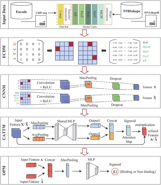
The architecture of our proposed model D-SSCA. The top part indicated the input data of D -SSCA. The second part ECDM is to converse sequence and shape profiles into feature matrix. The middle part is CNNM, which is useful to capture latent features from multi-dimensional biological profiles. The fourth part CATTM boosts the representation power by adaptive feature refinement. Finally, the bottom part OPM converts feature maps into final prediction.
In the following, we detail the four parts sequentially.
2.2.2 EnCoDing module
2.2.3 Convolutional neural network module
This module utilizes a parallel convolution layer and max-pooling layer to learn high-order representations for sequence and shape profiles, respectively. Besides, a dropout layer is employed to avoid over-fitting.
2.2.4 Channel ATTention module
To boost the representation power by learning some complex dependencies of high-order features alone channel dimension, a channel attention mechanism is leveraged [34]. Three steps are utilized to produce the output of channel attention mechanism when given a feature map P from CNNM.
2.2.5 OutPut module
The detailed settings for the presented D-SSCA model are shown in Table S3.
2.3 Baseline methods
We compare the presented D-SSCA method with various state-of-the-art TFBSs prediction approaches from two categories: (i) The solely sequence-based deep learning methods, such as DeepBind [18] and DanQ [20]. (ii) The deep learning methods combining sequence and shape, such as DLBSS [32] and CRPTS [33]. To perform a fair comparison, we meticulously optimize the above-mentioned methods and report the best results. The introduction of the methods is presented as follows:
DeepBind: This method is the first deep learning-based method for TFBSs prediction, composed of a convolutional layer, a max-pooling layer and a fully connected layer followed by a sigmoid function.
DanQ: This method is the variant of DeepBind, which is composed of a convolutional layer, a max-pooling layer, a Bi-LSTM layer and a fully connected layer followed by a sigmoid function.
DLBSS: This method leverages three Siamese convolutional layers to capture the common patterns from sequence and related shapes. Then, the captured features are concatenated to compute the final prediction.
CRPTS: This method is the variant of DLBSS. The difference between CRPTS and DLBSS is that CRPTS leverages a Siamese hybrid convolutional recurrent neural network to capture common patterns from sequence and related shapes.
2.4 Training algorithm and implements
2.4.1 Training algorithm

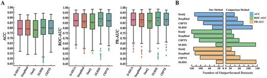
Performance comparison between D-SSCA and four comparison methods over 165 ChIP-seq datasets. (A) The ACC, ROC–AUC and PR–AUC of both D-SSCA and comparison methods, respectively. (B) The number of datasets which D-SSCA outperforms each comparison methods.
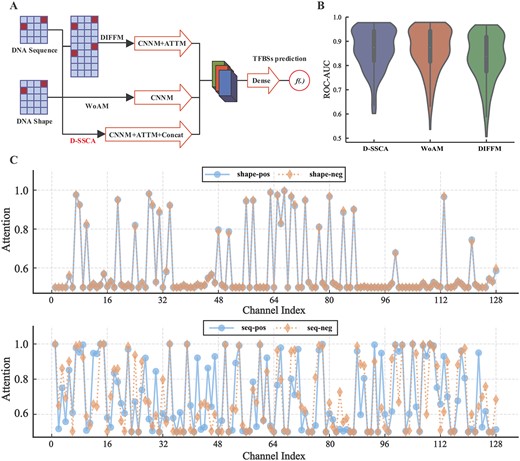
Performance comparison of variants of the presented D-SSCA model. (A) The brief description of variants. (B) The ROC-ROC of D-SSCA and related variants. The x-axis corresponds to the code of variants, and the y-axis corresponds to the ROC–AUC scores. (C) Activations induced by sequence-level channel attention module and shape-level channel attention module, respectively.
2.4.2 Implement of algorithm
Both our proposed model D-SSCA and baseline methods are implemented based on PyTorch. The optimization algorithm adopts PyTorch to implement Adam, with mini-batch set to 100 and other parameters set to the default. The proposed model utilizing Algorithm 1 learn 30 epochs, and obtain final model with best results by 5-fold cross-validation. Then, we confirm performance again by test sets.
2.5 Evaluation metric
In this paper, accuracy, ROC–AUC and PR–AUC are applied to measure the performance of our proposed model and baseline methods [36]. The summary of these metrics is as follows:
Accuracy: The accuracy refers to the proportion of predicted correct TBFSs and non-TBFSs over all samples. The ACC is used for short in subsequent sections.
ROC–AUC: This metric indicates the area under the receiver operating characteristic curve.
PR–AUC: This metric represents the area under the precision-recall curve.
3 Experimental results
Extensive studies are performed on ENCODE ChIP-seq datasets to thoroughly validate the utility of the presented D-SSCA model. More particularly, our studies mainly answer the following research questions:
RQ1: Can the presented D-SSCA model have better performance than several state-of-the-art TFBSs prediction methods? (Section Performance comparison)
RQ2: How do some important modules in the presented D-SSCA model affect the final performance, including the attention module and feature fusion strategy? (Section Ablation study)
RQ3: What is the relative importance of five shape profiles in human TFs-DNA recognitions? (Section Contribution analysis of DNA shape)
RQ4: Do both sequence and shape have common patterns across cell lines, and are these patterns helpful to further improve the final performance? (Section cross-cell lines TBFSs prediction)
3.1 Performance comparison (RQ1)
Figure 2 and Table S5 summarize the comparison results between our model and all the competitors over the 165 datasets in terms of ACC, ROC–AUC and PR–AUC. The main observations from Figure 2 and Table S5 are as follows:
The models with incorporating shape features consistently outperform those without incorporating shape features. The performance gain may lie in that most TFs bind to the corresponding genome positions by an interaction between base-pair readout and shape readout. Thus, an appropriate combination of sequence and shape features can improve the predictive power of deep learning models.
The presented D-SSCA model yields better performance than other comparison methods significantly with respect to average ACC, ROC–AUC and PR–AUC. This is mainly because the presented model considers the importance of shape features, and leverages the attention mechanism to adaptive refine the high-order features derived from sequence and shape profiles.
The variant models using Bi-LSTM such as DanQ and CRPTS perform worse than the models only using CNNs such as DeepBind and DLBSS, mainly because of the smaller window of the input sequence. This indicates that wider sequence context may provide the information of long-range dependency of motif variants, while narrower sequence may only provide local information of motifs.
Across most datasets, the DLBSS has better performance than the presented D-SSCA model with respect to ACC, ROC–AUC and PR–AUC. This reveals that the Siamese convolutional layers can simultaneously capture the common patterns from sequence and shape profiles, resulting in better generalization and stability. However, the parallel convolutional layers are helpful to discover the sequence motifs and shape motifs separately.
3.2 Model ablation (RQ2)
To better understand the utility of the attention module and the feature fusion strategy, we decompose the presented D-SSCA model with a set of variants. These variants are shown in Figure 3A and described as follows:
Without attention module (WoAM): This model is a variant of D-SSCA without considering the CATTM block.
Data-level feature fusion modelling: This model is a variant of D-SSCA without considering intermediate-level feature fusion, but leverages the data-level feature fusion to combine sequence and shape profiles.
Utility of attention module. We analyse the attention module for WoAM and D-SSCA, corresponding to the model without considering the attention module and our final model, respectively. As shown in Figure 3B and Table S6, the model with an attention module performs better on most datasets than that without an attention module. The relative improvement of D-SSCA over WoAM is 0.45% for ACC, 0.53% for ROC–AUC and 0.49% for PR–AUC, respectively. As we mentioned, several latent features related to TFs-DNA interaction should be captured more than other features. Therefore, the attention module is necessary for the presented D-SSCA model. This module helps our model to focus on critical latent features and suppress useless ones simultaneously.
To reveal how the attention module operates in practice and provide a clear picture of the function of the attention module, we analyze the distribution of the attention weights from the presented CATTM block. More specifically, we sample binding sites of Dnd41-CTCF, one of the most important binding proteins for transcription regulation, from the collected validation datasets. Then, we compute the average attention weights for all samples of Dnd41-CTCF and visualize the related distribution. Moreover, we compute the average attention weights of the corresponding negative samples for reference. The distribution of the attention maps is shown in Figure 3C. The observations about the role of attention operation are 2-folds. On the one hand, for high-order features from sequence profiles, the attention weights have specificity over several channels, demonstrating that various features from sequence profiles exhibit particular importance for TFBSs prediction. On the other hand, for high-order features from shape profiles, the attention weights are very similar over most channels, which indicates that shape-level attention is less important than sequence-level attention in performing feature refinement. To sum up, the presented CATTM block provides sequence-level specific responses for improving the performance of TBFSs prediction.
Utility of data-level fusion. We investigate the utility of data-level fusion on the completed datasets concerning ACC, ROC–AUC and PR–AUC, and report the performance of the model with data-level fusion and model with intermediate-level fusion. As shown in Figure 3B and Table S6, the model with intermediate-level feature fusion significantly outperforms the model with data-level feature fusion. This is mainly because some information implicit in raw samples may be redundancy and data-level feature fusion cannot fully utilize the complementary between multiple inputs, resulting in the limitation of prediction performance. Hence, the intermediate-level feature fusion is more appropriate for the presented D-SSCA model.
3.3 Contribution analysis of DNA shape (RQ3)
To investigate the importance of DNA shapes in TFs-DNA recognition, according to the publication [37], the presented D-SSCA model is adopted to infer the power of shape features in TFBSs prediction across the 165 ChIP-seq datasets. For individual datasets, D-SSCA is applied to identify TFBSs based on HelT, MGW, ProT, Roll, EP and the combination of five shapes referred to as shape combination. The performance increase of ROC–AUC is used to measure the feature importance.
Firstly, we construct a series of architectures by varying the number of convolutional kernels and the number of convolutional layers to study the impact of the model complexity on the representation ability of both sequence and shape features. A brief description of the architectures is shown in Table S4. The results demonstrated in Figure 4A indicate that the one-layer_128-kernels model yields the best performance concerning ROC–AUC. This reveals the importance of utilizing good convolutional kernels to capture high-order features from sequence and shape profiles. Therefore, all the studies carried out in this paper leverage the one-layer_128-kernels model.
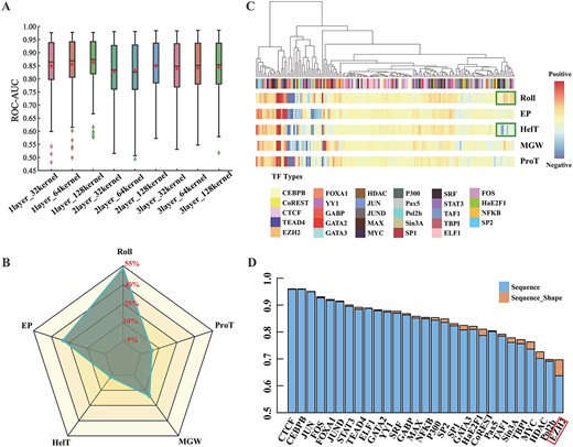
The contribution of DNA shape in TFBSs prediction. (A) The ROC–AUC of D-SSCA by varying the number of convolutional kernels and the number of convolutional layers. The x-axis corresponds to the code of variants, and the y-axis corresponds to the ROC–AUC scores. (B) The overall contribution of Roll, EP, HelT, MGW and ProT in TBFSs prediction. (C) The detailed analysis of the contribution of each shape on the 165 ChIP-seq datasets. Each column in the heatmap refers to one ChIP-seq dataset. These columns are organized by hierarchical clustering. The green boxes represent the ChIP-seq dataset where the contribution of Roll and HelT is reversed. (D) The ROC–AUC comparison between D-SSCA based on sequence+shape and D-SSCA only based on the sequence. The red box represents the category of TF with the most significant ROC–AUC improvement when combining sequence and shape compared to only using sequence information.
Then, we analyze the prediction performance of adopting individual shape features to assess how individual shape features contribute to the TBFSs identification. The results demonstrated in Figure 4B indicate that Roll, EP, HelT, MGW and ProT contribute 53.3, 30.2, –3.1, 15.6 and 4.00%, respectively. This is mainly because inter-base pair shapes (Roll and HelT) may be redundant on several ChIP-seq datasets. In contrast, the intra-base pair shapes (EP, MGW and ProT) may be complementary to each other and helpful to improve the predictive power.
After that, we cluster the prediction fractions to measure the contribution of shape features across individuals from the 165 ChIP-seq datasets. The results demonstrated in Figure 4C indicate that Roll and HelT have reverse contributions on several ChIP-seq datasets, proving the conclusion depicted in Figure 4B. Besides, five shapes tend to contribute positively to most ChIP-seq datasets, suggesting each shape is essential in TBFSs recognition. Surprisingly, all five shapes make a negative contribution to the prediction of some TFBSs, which reveals that the binding mechanism of some TFs is not specific of shape in some cells, but sequence or other factors specific.
Finally, we compare the performance between the model with the utility of both sequence and shape features and the model with the only utility of sequence features to explore whether the combination of five shapes can contribute to predicting each category of TFBSs. Figure 4D indicates that the ROC–AUC performance is significantly improved among all ChIP-seq datasets of 29 TFs by combining five shape features. This justifies that for one specific TF, the average positive contrition of five shapes is greater than the average negative contribution.
Moreover, the maximum and the average performance improvements are 0.05 and 0.01, respectively, revealing that various TFs have different shape-level binding preferences. Notably, EZH2 achieves the best performance boost by combining sequence and five shapes, but the biological mechanism remains obscure.
3.4 Cross-cell lines TBFSs prediction (RQ4)
To investigate the occupancy of common patterns of both sequence and shape across cell lines, and validate the utility of the presented D-SSCA model to learn the universal rule of a specific TF in various cell lines, we conduct a series of studies, including the followings:
First, for a specific TF, the presented D-SSCA model is constructed on other cell lines, and then used to predict TFBSs in the cell line of interest. The ChIP-seq datasets from GM12878, K562, Helas3 and Hepg2 cells are adopted in this study, because as shown in Figure 5A, most TFs across these cells are overlapped. As shown in Figure 5B, the average ROC–AUC of cross-cell line prediction is more than 0.8. However, across most datasets, the performance of the cross-cell line prediction is worse than the conventional prediction. This phenomenon indicates that the cell line-specific factors have dominant roles for TFs-DNA recognition, whereas the cell line-independent factors only play a supplementary role.
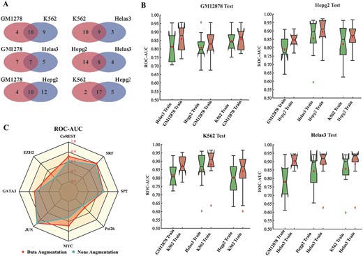
Performance of cross-cell line TFBSs prediction. (A) The overlap of TFs across GM12878, K562, Helas3 and Hepg2 cells. (B) The ROC–AUC comparison between cross-cell line prediction and conventional prediction. The cross-cell line prediction indicates that D-SSCA is constructed on other cell lines, and then used to predict TFBSs in the cell line of interest. (C) The ROC–AUC comparison between data augmentation and none augmentation. The data augmentation refers that D-SSCA is constructed using the universal dataset.
Furthermore, to study the availability of the presented D-SSCA model to simultaneously capture cell line-specific factors and cell line-independent factors cross-cell lines, CoREST, EZH2, GATA3, JUN, MYC, Pol2b, SP2 and SRF are selected form the ChIP-seq datasets. The D-SSCA model is constructed on the universal dataset. Considering a specific TF, the universal dataset is composed of all samples from different cell lines. As shown in Figure 5C, prediction using universal dataset has better performance than conventional prediction on the entire datasets except for CTCF. This observation demonstrates that the performance of D-SSCA can be further improved by learning cell line-specific factors and cell line-independent factors cross-cell lines. Besides, sequence and shape features may have common interplay patterns across various cell lines. Nevertheless, whether shape features are cell line-specific factors or cell line-independent factors now await validation.
4 Discussion
Here, we develop a convolution attention-based method, named D-SSCA, to predict TFBSs by jointly combining sequence and shape profiles. There have been several attempts to incorporate attention mechanism to improve the predictive power of CNNs in TFBSs prediction by assigning of more importance on the actual TFBSs in the input sequence. However, aforementioned studies only focus on capturing spatial correlations between features. To this end, we leverage the channel mechanism to boost the representation power of D-SSCA by learning the complex inter-channel dependency of various latent features.
To validate the utility of the presented method, many studies are conducted on ENCODE ChIP-seq datasets. Experimental outcomes demonstrate that the presented D-SSCA can consistently outperform several state-of-the-art methods in TFBSs prediction. Besides, the attention module is proven to realize refinement along channel dimension for high-order features derived from sequence profiles. More surprisingly, the attention module is less important in providing refinement for high-order features derived from shape profiles than sequence profiles. Therefore, in the downstream application, the shape-level attention module could be removed to reduce the parameter count with only a marginal decrease of performance.
Furthermore, this study leads to the comprehensive analysis of five shape profiles, including HelT, MGW, ProT, Roll and EP. The results support the hypothesis that and the role of sequence and shape information in determination TFs-DNA binding is complementary and integration of sequence and shape features can improve the predictive power of TFBSs. Beyond aforementioned hypothesis, the observations also indicate that shape profiles are not complemented to each other on several datasets, suggesting that more sophisticated shape-shape interaction mechanisms may occur beyond sequence-shape interplay.
This study still faces several limitations: First, the specificity of TFs-DNA binding is influenced by multiple factors, such as chromatin accessibility [38], histone modifications [39] and nucleosome occupancy [40]. Considering only sequence and shape profiles is insufficient to interpret the TFs-DNA binding in vivo and in vitro [41]. Hence, we plan to further study other factors in the future. Second, we mainly focused on investigating cell line-specific and cell line-independent factors, future work is needed to further research the tissue-specific and tissue-independent factors.
To sum up, our study provides an innovative deep learning-based method for inferring potential TFBSs, and revealing biological mechanism of shape-mediated TFs-DNA binding behavior. To facilitate future researches, the source code for running the presented D-SSCA model is available at https://github.com/MoonLord0525/.
The TFs-DNA binding mechanism is an important part of the cis-regulatory code, yet remains elusive. Hence, how to predict putative TFBSs has become the fundamental issue in bioinformatics.
We present a valuable convolution attention model for TFBSs prediction by the combination of sequence and shape. This method is found to perform better compared with several state-of-the-art methods. More intriguingly, the attention module can be interpreted by weight map visualization.
Extensive analysis indicate that shape profiles have positive contribution over most datasets and demonstrate the occupancy of common patterns of sequence-shape interplay.
The source codes and data are released at https://github.com/MoonLord0525/ to facilitate future research in this direction.
Acknowledgments
This work is supported by the National Natural Science Foundation of China under (Grant Nos. 61922020, 61702058); the China Postdoctoral Science Foundation funded project (No. 2017M612948).
Yongqing Zhang is an associate professor in the School of Computer Science at the Chengdu University of Information Technology. He is a senior member of CCF. His research interests include machine learning and bioinformatics.
Zixuan Wang is a graduate student in the School of Computer Science at the Chengdu University of Information Technology. His research interests include deep learning and bioinformatics.
Yuanqi Zeng was a graduate student in the School of Computer Science at the Chengdu University of Information Technology. His research interest includes deep learning and bioinformatics.
Yuhang Liu is a graduate student in the School of Computer Science at the Chengdu University of Information Technology. His research interests include deep learning and bioinformatics.
Shuwen Xiong is a graduate student in the School of Computer Science at the Chengdu University of Information Technology. His research interests include deep learning and bioinformatics.
Maocheng Wang is a graduate student in the School of Computer Science at the Chengdu University of Information Technology. His research interests include deep learning and bioinformatics.
Jiliu Zhou is a professor in the School of Computer Science at the Chengdu University of Information Technology. His research interests include intelligent computing and image processing.
Quan Zou is a professor in the Institute of Fundamental and Frontier Science at the University of Electronic Science and Technology of China. He is a senior member of IEEE and ACM. His research interests include bioinformatics, machine learning and algorithms.
