


Abstract
The discovery of cancer subtypes has become much-researched topic in oncology. Dividing cancer patients into subtypes can provide personalized treatments for heterogeneous patients. High-throughput technologies provide multiple omics data for cancer subtyping. Integration of multi-view data is used to identify cancer subtypes in many computational methods, which obtain different subtypes for the same cancer, even using the same multi-omics data. To a certain extent, these subtypes from distinct methods are related, which may have certain guiding significance for cancer subtyping. It is a challenge to effectively utilize the valuable information of distinct subtypes to produce more accurate and reliable subtypes. A weighted ensemble sparse latent representation (subtype-WESLR) is proposed to detect cancer subtypes on heterogeneous omics data. Using a weighted ensemble strategy to fuse base clustering obtained by distinct methods as prior knowledge, subtype-WESLR projects each sample feature profile from each data type to a common latent subspace while maintaining the local structure of the original sample feature space and consistency with the weighted ensemble and optimizes the common subspace by an iterative method to identify cancer subtypes. We conduct experiments on various synthetic datasets and eight public multi-view datasets from The Cancer Genome Atlas. The results demonstrate that subtype-WESLR is better than competing methods by utilizing the integration of base clustering of exist methods for more precise subtypes.
Introduction
Cancer is a complex and diverse disease, whose heterogeneity makes precise treatment imperative. This can be accomplished by dividing cancer patients into different subtypes [1]. There is an increasing demand to identify cancer subtypes by analyzing cancer-related genomic data.
The development of high-throughput technologies makes various genomic data from large-scale projects such as The Cancer Genome Atlas (TCGA) [2] available. TCGA provides heterogeneous omics data including gene expression, miRNA expression and DNA methylation from the same sample for over 30 cancers, which offers unprecedented opportunities to study the occurrence and development of cancer. Studies have shown that single data types such as gene expression can merely describe a biological process at one specific molecular level, provide incomplete information for subtypes and cannot capture the subtleties of the cancer [3–5].
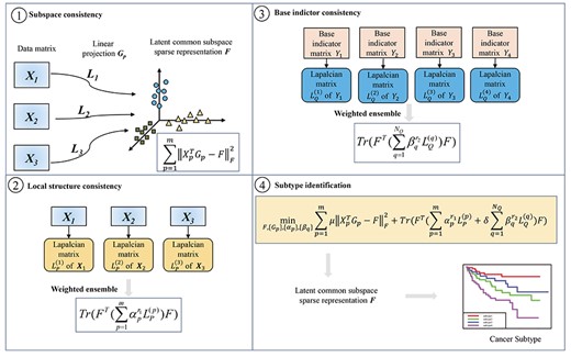
Workflow of subtype-WESLR. Matrix |$X_p$|(|$p$|=1,...,3) and |$Y_q$|(|$q$|=1,...,4) are the inputs. Subtype-WESLR projects each sample feature profiles from each data type to a common latent subspace corresponding to subspace consistency, which should keep the local structure of the original sample feature space and be consistent with the weighted ensemble clustering, i.e. maintaining local structure consistency and base indictor consistency, and optimizes |$F$| by an iterative method. The matrix |$F$| can be used for cancer subtype identification. For each row in matrix |$F$|, the column with the maximum value is the cluster index of a cancer subtype.
Distinct data types from various biological domains provide a different, partly independent and complementary view of the genome. Thus, many computational methods integrate multi-omics data to discover cancer subtypes [6, 7]. Early integration of multi-omics data is directly concatenating multiple-omics data [8]. For example, LRAcluster [8] concatenates multiple heterogeneous omics data for each sample by probabilistically modeling the distribution of numeric, count and discrete features, but this integration does not consider different distributions of data in the different omics and the curse of dimensionality. One common strategy to combine biological data is to cluster each data type independently and integrate their different cluster assignments [9–11]. For example, PINS [10] merges connectivity matrices into a combined patients similarity matrix by building a sample connectivity matrix for each data type. However, this integration ignores the weak but consistent correlations across data types.
Some statistical methods [12–14] model the distribution of each data type and then maximize the likelihood of multi-omics data. The iClusterBayes [14] method captures the inherent structure of multiple omics data by using a few Bayesian latent variables to achieve joint dimension reduction. However, these methods are limited by strong assumptions on multi-omics data. Moreover, feature selection is also required for these methods because of the high number of features. Similarity-based approaches [15–17] for multi-omics data avoid this problem. For example, similarity network fusion (SNF) builds a sample-similarity network for each omic and fuses these sample networks into a single combined network based on message passing [15].
Some methods [18, 19] consider the integration of multi-omics data with joint dimensionality reduction. Pattern fusion analysis (PFA) [19] fuses local sample pattern from each data type into an integrated sample pattern corresponding to phenotypes by an adaptive optimization strategy. Deep learning also has been applied to molecular data processing and analysis [20, 21]. Subtype-GAN [21] utilizes a multiple-input-multiple-output neural network to accurately model complex omics data and uses consensus clustering and a Gaussian mixture model to identify tumor samples’ molecular subtypes.
Owing to the uncertainty of subtypes, methods may have different subtypes for the same cancer, even using the same multi-omics data, which have certain guiding significance for cancer subtyping. How to effectively utilize the valuable information of distinct subtypes poses a challenge to produce more accurate and reliable subtypes. Ensemble methods can utilize some preselected clustering methods to obtain better clustering results [22–25]. In ClustOmics [25], each input clustering method constructs a graph by computing the support edge of each pair of parents nodes, and an integration graph is constructed by integrating these graphs and applied to graph clustering based on Modularization Quality [26].
Based on the sparse subspace learning framework [27–29], we propose an ensemble clustering approach called weighted ensemble sparse latent representation of multi-view data for subtype discovery (subtype-WESLR) (Figure 1), which identifies cancer subtypes by analyzing multiple heterogeneous omics data and simultaneously taking some cancer subtyping of other methods into account. Our model projects each sample feature profile from each data type to a common latent subspace corresponding to subspace consistency, which should keep the local structure of the original sample feature space and be consistent with the ensemble clustering, i.e. maintaining local structure consistency and base indictor consistency, and optimizes the common subspace by an iterative method to identify cancer subtypes. Different from other ensemble methods, in which different clustering algorithms are applied on each view, respectively, or base partitions of distinct clustering algorithms are treated equally, subtype-WESLR directly applies clustering algorithms to multi-view data to obtain base clustering as prior knowledge. Moreover, a weight ensemble is adaptively applied to distinct base clustering for the optimum combination. To verify the effectiveness of subtype-WESLR, we conducted experiments on various synthetic datasets as well as eight public multi-view datasets from TCGA. Experimental results demonstrate that subtype-WESLR outperforms competing methods and weighted ensemble clustering can lead to more accurate and reliable subtypes for subtype discovery.
To summarize, our contributions are as follows:
(i) We consider weighted ensemble clustering of different methods, aiming at utilizing valuable information of identified distinct subtypes as prior knowledge, to produce more precise subtypes.
(ii) We develop subtype-WESLR to learn sparse latent representation among multi-view data for subtype discovery, by assuming that the input views are generated from the common latent representation. To maintain the local structure consistency of each data type and indictor consistency of weighted ensemble clustering, we introduce multi-view Laplacian regularization.
(iii) Experiments on synthetic data demonstrate superiority of subtype-WESLR on discovering common patterns under different noise and distinct numbers of base clustering. Experiments on eight public multi-view datasets from TCGA datasets show that subtype-WESLR captures more reliable subtypes than competing methods in cancer subtype discovery.
Methods
Cancer is a complex disease affected by many factors. Distinct data types provide a different, partly independent and complementary view of the genome. It is helpful to find the common information of features from different perspectives for subtype identification. Subspace learning-based algorithms aim to learn a latent subspace shared with multiple views by assuming that the input views are generated from this latent subspace. Based on the sparse subspace learning framework, we propose subtype-WESLR. In this section, we will give the details about our proposed method.
Problem formalization
Sparse latent representation of multi-view data
Suppose we have |$n$| samples (e.g. patients) and |$m$| views (e.g. miRNA, mRNA, DNA methylation). The |$p$|-th view data are denoted as matrix |$ X_p \in R^{d_p \times n} $||$(p=1,2,{\ldots },m)$|, where |$d_p$| is the number of features in |$p$|-th feature matrix.
Local structure consistency of multi-omics data
By combining multiple view data, the shared sparse latent subspace should preserve the local structure of the original feature space, and multi-view Laplacian regularization can be used to maintain the local consistency.
Base indictor consistency of distinct clustering
To a certain extent, subtypes from distinct methods are related for the same cancer, which have certain guiding significance for cancer subtyping. Integration of base clustering can be meaningful for subtype discovery.
Weighted ensemble sparse latent representation
Solution of subtype-WESLR
Applying the update rules (11)–(14), we show that the optimization of subtype-WESLR is convergent. This is proved in the supplementary material. When the objective function (10) is solved by applying subtype-WESLR, the indication matrix |$F$| can be used for cancer subtype identification, where the column of the maximum value for each row in matrix |$F$| is the cluster index of a cancer subtype. Also, |$\{{\alpha }_p\}_{p=1}^{m}$| and |$\{{\beta }_q\}_{q=1}^{N_Q}$| reflect the contribution of each view feature matrix and each base clustering algorithm to the prediction, respectively.
Based on the above optimization process, we summarize subtype-WESLR in Algorithm 1.

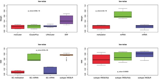
Analysis on synthetic data. (A) Contribution of base clustering to subtype-WESLR. |$P$|-value |$={6.58\times 10^{-16}}$| indicates the significant difference between LRAcluster and SNF by two-sample t-test. (B) Contribution of DNA methylation, miRNA and mRNA profile to subtype-WESLR. |$P$|-value |$={2.2\times 10^{-16}}$| indicates the significant difference between methylation and miRNA by two-sample t-test. (C) Value of NMI among SC-methylation, SC-miRNA, SC-mRNA and subtype-WESLR using SC-methylation, SC-miRNA and SC-mRNA as base clustering. |$P$|-value |$={8.23\times 10^{-6}}$| indicates the significant difference between SC-miRNA and subtype-WESLR by two-sample t-test. (D) Value of NMI on subtype-WESLR under distinct numbers of base clustering. |$P$|-value |$={.00883}$| indicates the significant difference between subtype-WESLR(3) and subtype-WESLR(3) by two-sample t-test. Experiments were carried out 50 times to generate datasets containing 0%, 20% and 30% extra noise, i.e. low, moderate and high noise, respectively.
Performance of distinct methods on synthetic data. Best results are in boldface.
| Method | Low noise | Moderate noise | High noise |
|---|---|---|---|
| NEMO | 0.56 |$\pm $| 0.14 | 0.57 |$\pm $| 0.17 | 0.49 |$\pm $| 0.16 |
| PFA | 0.18 |$\pm $| 0.08 | 0.18 |$\pm $| 0.06 | 0.14 |$\pm $| 0.06 |
| iClusterBayes | 0.53 |$\pm $| 0.21 | 0.46 |$\pm $| 0.20 | 0.42 |$\pm $| 0.17 |
| moCluster | 0.40 |$\pm $| 0.09 | 0.41 |$\pm $| 0.05 | 0.42 |$\pm $| 0.03 |
| iClusterPlus | 0.42 |$\pm $| 0.12 | 0.49 |$\pm $| 0.07 | 0.44 |$\pm $| 0.08 |
| LRAcluster | 0.46 |$\pm $| 0.17 | 0.46 |$\pm $| 0.15 | 0.53 |$\pm $| 0.17 |
| SNF | 0.72 |$\pm $| 0.15 | 0.67 |$\pm $| 0.03 | 0.65 |$\pm $| 0.05 |
| subtype-WESLR | 0.77|$\pm $|0.13 | 0.74|$\pm $|0.07 | 0.68|$\pm $|0.07 |
Results
Experimental settings
Parameter settings. To compute the Laplacian matrix, the two free parameters |$k$| and |$\theta $| have reasonable ranges {10,15,20,25,30,35} and {0.1,0.2,0.3,0.4,0.5,0.6,0.7,0.8,0.9,1}, respectively. The regularization parameters |$\mu $| and |$\lambda $| are in the range {0.0001,0.001,0.01,0.1,1,10} and {0.001,0.01,0.1,1,10} separately. Parameters |$r_1$|, |$r_2$| and |$\sigma $| are related to the weight coefficients |${\alpha }_p$| and |${\beta }_q$|, and |$r_1$| and |$r_2$| are in the range {2,3,5,10,100,1000}, where smaller values have better performance. The parameter |$\sigma $| is in the range {0.1,1,10,100,1000,10000}, and |${\alpha }_p$| and |${\beta }_q$| can be close to |$1/m$| and |$1/{N_Q}$| when |$\sigma $| is very large. The regularization parameter |$\delta $|, which balances the weight between feature matrices and base clustering algorithms, is in the range {0.00001,0.0001,0.001,0.01,0.1,1}. Owing to the convergence of subtype-WESLR, the stopping rules are set to |$\frac{\Vert{(G_p)}_{t+1}-{(G_p)}_{t}\Vert }{\Vert{(G_p)}_{t}\Vert } \leq 10^{-5}$| or the maximum number of iterations.
Competing methods. We compared subtype-WESLR with related multi-view clustering methods including SNF [15], iClusterPlus [13], LRAcluster [8], moCluster [18], PFA [19], iClusterBayes [14], kmeans [30], spectral clustering [31] and NEMO [17] on synthetic data and TCGA data. We also compared subtype-WESLR with the recent ClustOmics [25] and subtype-GAN [21] on TCGA data.
Evaluation metrics. The normalized mutual information [22], namely NMI, which measures the concordance of two clusterings, was used to evaluate the performance on simulated datasets. The value of NMI is between 0 and 1, and a higher value is better. We compared the performance of subtype-WESLR and other approaches by the P-value and the concordance index (C-index) of the Cox regression model on eight cancer cohorts and analyzed the identified subtypes by survival analysis. It is worth noting that for each method, we set parameters according to the rules in its paper and conducted many tests with different settings on our simulated data or real data, attempting to choose the relatively better NMI or |$P$|-value. The results in our work may be different from their reports due to difference in data and parameter settings.
Time complexity. The running time of subtype-WESLR can be separated into calculating graph Laplacian matrix step and optimization step. Calculating the graph Laplacian matrix in all base clustering methods and all omics require |$O(n^2 \cdot N_Q)$| and |$O({d_p}^2 \cdot m)$|, respectively. The optimization can be computed in time |$O(T \cdot (N_Q+m))$| during iterative process, in which |$T$| represents the maximum number of iterations. Therefore, the total time complexity is |$O(n^2 \cdot N_Q + {d_p}^2 \cdot m + T \cdot (N_Q+m))$|.
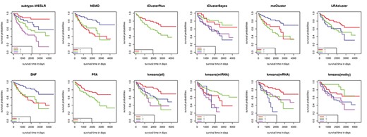
Kaplan–Meier survival curves of KIRC for subtype-WESLR, NEMO, iClusterPlus, iClusterBayes, moCluster, LRAcluster, SNF, PFA, kmeans (all), kmeans (miRNA), kmeans (mRNA) and kmeans (methy).
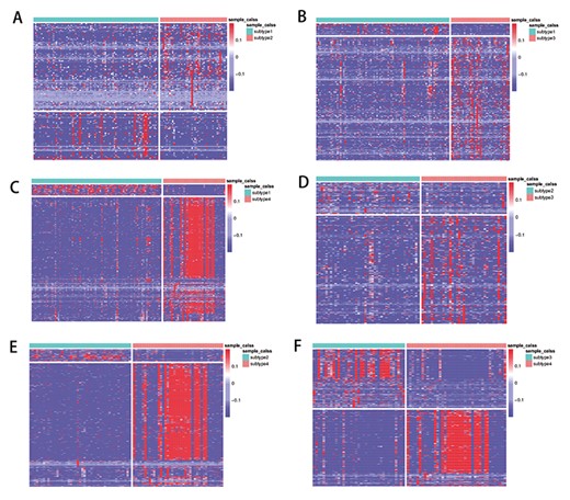
Heatmaps of significantly differential expressed mRNA among KIRC subtypes. (A) Subtypes 1 and 2; (B) subtypes 1 and 3; (C) subtypes 1 and 4; (D) subtypes 2 and 3; (E) subtypes 2 and 4; (F) subtypes 3 and 4. Each row represents a genomic feature, and each column represents a sample.
Analysis on synthetic data
We compared subtype-WESLR with other methods based on the synthetic datasets [18, 19] involving miRNA, mRNA and DNA methylation. Multi-view data were separately produced from real genomic profiles GSE73002 [32], GSE10645 [33] and GSE51557 [34] for miRNA expression, mRNA expression and DNA methylation data, as explained by singular value decomposition in the supporting information of Shi et al. [19]. Owing to the better performance of good-condition numeric examples over bad-condition, synthetic data were simulated in bad-condition with |${mean}^s \in \{0,0.25,0.5,0.75\}$|, including 200 samples with four ground-truth clusters as 1–50, 51–100, 101–150 and 151–200. Each data type can discriminate incomplete clusters, and all of the data types correspond to clusters {1–50, 51–150, 151–200}, {1–50/101–150, 51–100, 151–200} and {1–100, 101–150, 151–200}. Besides, SNF, iClusterPlus, LRAcluster and moCluster were used as base methods of subtype-WESLR, i.e. the clustering of base methods were inputs of subtype-WESLR. Experiments on simulated datasets demonstrate that our method is robust to a variety of parameter settings (Supplementary Figures S1–S6).
Comparison across distinct extra noise. Experiments were carried out 50 times to generate datasets containing 0%, 20% and 30% extra noise, i.e. low, moderate and high noise, respectively. In the simulation, we considered the NMI between the clusters obtained by distinct methods and the ground-truth clusters (Table 1; Supplementary Figure S7A). As shown in Table 1, subtype-WESLR is superior to other methods, in terms of concordance with ground-truth clusters across diverse noise settings, and there is only small fluctuation as extra noise increases. NEMO and iClusterBayes have also been relatively stable under different noise levels. PFA performs worst, probably because the algorithm is sensitive to parameters.
Survival analysis of distinct methods on TCGA data. Negative |${log}_{10} P$|-value of log-rank test is used for statistical significance test. Numbers of clusters are in parentheses. Best results are in boldface.
| Cancer type | KIRC | BRCA | COAD | SKCM | GBM | LUSC | LIHC | OV |
|---|---|---|---|---|---|---|---|---|
| NEMO | 4.48 (3) | 0.310 (4) | 0.959 (4) | 2.74 (4) | 2.96 (3) | 2.15 (3) | 1.60 (3) | 0.0506 (3) |
| iClusterPlus | 1.92 (2) | 2.14 (5) | 1.04 (4) | 1.10 (4) | 0.824 (3) | 0.921 (3) | 0.569 (3) | 1.59 (3) |
| iClusterBayes | 2.51 (4) | 1.06 (5) | 0.886 (4) | 1.85 (4) | 0.215 (3) | 1.24 (3) | 1.11 (3) | 1.48 (3) |
| moCluster | 2.82 (3) | 3.31 (5) | 1.04 (3) | 2.96 (4) | 1.96 (3) | 2.31 (3) | 1.02 (2) | 1.60 (3) |
| LRAcluster | 2.07 (3) | 2.23 (5) | 1.17 (4) | 3.25 (3) | 2.00 (3) | 2.35 (3) | 0.387 (3) | 2.96 (3) |
| SNF | 3.40 (3) | 2.82 (4) | 1.07 (3) | 2.31 (4) | 2.92 (3) | 2.03 (3) | 1.54 (3) | 1.15 (3) |
| PFA | 2.08 (2) | 2.89 (5) | 1.00 (3) | 2.64 (4) | 2.23 (2) | 1.04 (3) | 2.64 (2) | 0.0506 (3) |
| kmeans (miRNA) | 1.52 (4) | 1.15 (4) | 0.638 (3) | 0.456 (3) | 0.00877 (3) | 0.409 (3) | 1.04 (3) | 0.0269 (3) |
| kmeans (mRNA) | 1.80 (4) | 2.62 (5) | 1.05 (3) | 1.14 (3) | 0.0132 (3) | 1.46 (3) | 2.07 (3) | 0.509 (3) |
| kmeans (methy) | 2.05 (4) | 0.409 (5) | 0.0458 (3) | 0.538 (3) | 0.337 (3) | 1.57 (3) | 0.0362 (3) | 0.377 (3) |
| kmeans (all) | 2.21 (4) | 2.54 (5) | 0.26 (3) | 1.03 (3) | 0.77 (3) | 0.495 (3) | 0.119 (3) | 1.41 (3) |
| subtype-WESLR | 4.76 (4) | 5.24 (5) | 2.43 (4) | 5.00 (5) | 3.84 (3) | 2.30 (5) | 5.21 (4) | 3.44 (3) |
Better performance means greater contribution. As a method of base clustering in subtype-WESLR, SNF was not sensitive to extra noise and was second to subtype-WESLR. LRAcluster was better and more stable with noise over moCluster and iClusterPlus, which both were poor in identifying clusters. Performances of these base methods correspond to contributions of base clustering to subtype-WESLR, i.e. better performance of a base method indicates greater contribution of base clustering to subtype-WESLR in Figure 2A, and SNF contributed the most. Similarly, Figure 2B shows contributions of DNA methylation, miRNA and mRNA to subtype-WESLR. Compared with DNA methylation and mRNA, miRNA had the greatest effect on subtype-WESLR.
Multi-omics data versus single-omic data. Spectral clustering [31] was applied separately to DNA methylation, miRNA and mRNA named as SC-methylation, SC-miRNA and SC-mRNA, respectively, to generate base clustering that subtype-WESLR used as inputs. Figure 2C shows that integration of multi-omics data is more stable comparing with one single data type, and miRNA is more useful to discover clusters over DNA methylation and mRNA, agreeing with the observation of Figure 2B, even if different base methods are employed by subtype-WESLR. As miRNA has advantages over mRNA and DNA methylation in spectral clustering, we made experiments on miRNA among moCluster, iClusterPlus, LRAcluster, spectral clustering and subtype-WESLR that utilizes the above methods as base methods (Supplementary Figure S7B). SNF is not used as the basic method because it is not applicable to single data type. Results illustrate that subtype-WESLR is also suitable for dealing with single data type. We also applied subtype-WESLR to data by combining any two of DNA methylation, miRNA and mRNA, named as subtype-WESLR (mRNA+miRNA), subtype-WESLR (methy+miRNA) and subtype-WESLR (methy+mRNA), respectively. In subtype-WESLR (mRNA+miRNA), SC-miRNA and SC-mRNA were used as base methods. Subtype-WESLR (methy+miRNA) and subtype-WESLR (methy+mRNA) take similar approach, and subtype-WESLR (methy+mRNA+miRNA) employs SC-mRNA, SC-methylation and SC-miRNA as base methods. Supplementary Figure S7C shows that subtype-WESLR performs better on three data types compared with any combination of two data types and indicates that integrating more multi-omics data of high quality can be more helpful for capturing common patterns. Therefore, weighted ensemble base clustering on multiple omics data can lead to a more stable clusters using subtype-WESLR.
Performances of subtype-WESLR under distinct numbers of base clustering. We also discussed the effectiveness of subtype-WESLR when distinct numbers of base clustering were treated as inputs (Figure 2D). As shown in Supplementary Figure S7D and E, subtype-WESLR(2) employs moCluster and iClusterPlus as base methods, whereas subtype-WESLR(3) also utilizes LRAcluster in addition to moCluster and iClusterPlus, owing to the performance of LRAcluster superior to moCluster and iClusterPlus. In the full model, i.e. subtype-WESLR, we used SNF, moCluster, iClusterPlus and LRAcluster as base methods. Figure 2D demonstrates that subtype-WESLR is superior to subtype-WESLR(2) and subtype-WESLR(3), which implies a well-performing base clustering helps improve the performance of subtype-WESLR.
Various experiments on synthetic data showed the superiority of subtype-WESLR on discovering common patterns of multi-view data. Finally, we studied the consistency of obtained subtypes (Supplementary Figure S8). Results illustrate that subtype-WESLR can identify consistent subtypes on synthetic data each time.
Analysis on TCGA data
Recently, mRNA is the most common and widely used in multi-omics data, to identify cancer subtypes by differentially expressed gene expression profiles. MicroRNAs are small noncoding RNAs that can cause the degradation of target gene mRNA or inhibit its translation by complementary pairing with the specific base of target gene mRNA and widely negatively regulate the expression of target gene. If the relevant miRNA mutates, activates the expression of relevant oncogenes or causes the deletion of tumor suppressor genes, it will lead to tumor. DNA methylation closely regulates gene expression. High DNA methylation often occurs in the promoter region of tumor suppressor gene, whereas low DNA methylation occurs in the promoter region of oncogene. Therefore, abnormal DNA methylation is usually used as an important molecular marker for tumor diagnosis, classification and treatment. These distinct data types provide a different, partly independent and complementary view of the genome. Studies show that it is helpful to integrate these multi-omics data for subtype identification [8, 15, 17, 19].
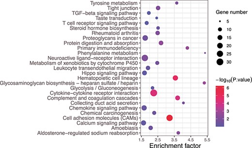
KEGG signal pathway enrichment analysis of differentially expressed mRNA on KIRC. The x-axis is the enrichment factor, which indicates the ratio of the proportion of proteins annotated to this pathway in the differentially expressed proteins to the proportion of proteins annotated to a certain pathway in the species. The larger the enrichment factor, the more reliable the enrichment significance of differential proteins in this pathway. The y-axis represents the KEGG path, and the path name is shown at the left vertical axis. The size and color of a dot represent the number of genes enriched in this pathway and the level of the |$P$|-value, respectively.
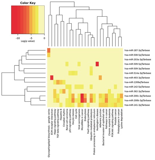
Significant signaling pathways about the differentially expressed miRNAs by utilizing the DIANA-miRPath.
We applied subtype-WESLR to eight publicly available multi-view datasets from TCGA, arranged and provided by [7]. These are Kidney Renal Clear Cell Carcinoma (KIRC), Breast Invasive Carcinoma (BRCA), Colon Adenocarcinoma (COAD), Skin Cutaneous Melanoma (SKCM), Lung Squamous Cell Carcinoma (LUSC), Glioblastoma Multiforme (GBM), Ovarian Serous Cystadenocarcinoma (OV), and Liver Hepatocellular Carcinoma (LIHC). Samples in each tumor dataset contain the following data types: miRNA expression, mRNA expression, DNA methylation and clinical profiles. Data preprocessing and normalization were performed to improve experimental results. Samples with more than |$20\%$| missing data of each data type were removed. Similarly, features with more than |$20\%$| missing data across samples were abandoned. We performed normalization provided by [15], and finally obtained 206 samples in KIRC, 623 in BRCA, 214 in COAD, 439 in SKCM, 271 in GBM, 337 in LUSC, 404 in LIHC and 290 in OV. As genomic data are largely redundant, Principal Component Analysis (PCA) was used for each data type, respectively, while maintaining |$95\%$| information before data integration. How to identify the number of subtypes is crucial for cancer subtype discovery. Since comparison methods have different criteria to determine the optimal number of subtypes, we did not require the same number of subtypes for each methods. We adopted the silhouette width[35] to determine the optimal number of clusters in subtype-WESLR, which is also is used in [15, 16, 19]. The silhouette width is an evaluation index of the density and dispersion of clusters, which is between - 1 and 1. The closer the value is to 1, the better the clusters are. Supplementary Figure S9 shows that four subtypes in KIRC, five in BRCA, four in COAD, five in SKCM, three in GBM, five in LUSC, four in LIHC and three in OV could be obtained according to the silhouette index. moCluster, LRAcluster, SNF and PFA were utilized as base method of subtype-WESLR for TCGA data. We did not consider identified subtypes with clusters of size below 10 across each methods. Supplementary Figures S10–S15 illustrate how to select parameters for KIRC.
Comparison with previous studies on eight cancer cohorts. As shown in Table 2, subtype-WESLR discovers subtypes with more significant survival differences for eight cancer cohorts in most case. Meanwhile, values of the C-index by different methods on TCGA data were shown in Supplementary Table S1. Results indicated that subtype-WESLR could obtain the higher value of C-index in accordance to the P-value in most case. Kmeans was also applied separately to DNA methylation, miRNA, mRNA and the combined data by concatenating the above three data types named as kmeans (methy), kmeans (miRNA), kmeans (mRNA), and kmeans (all), respectively. Table 2 demonstrates that integration of multi-omics data is more advantageous compared with one single data type. Note that none of competing methods can identify subtypes with more significant than subtype-WESLR in most case, which shows an advantage of subtype-WESLR over other methods. |$-{log}_{10}P$|-value of NEMO on KIRC is 4.48, second after subtype-WESLR. However, subtypes 1 and 2 of NEMO cannot be well discriminated. The |$P$|-values for BRCA and COAD by NEMO do not reach 0.01, in accordance with the results in NEMO itself. The superiority of subtype-WESLR over moCluster, LRAcluster, SNF and PFA for each cancer shows that subtype-WESLR can use poor base clustering results to achieve more reliable clustering. We also reported the results of subtype-WESLR with ClustOmics and subtype-GAN in their own work (Supplementary Table S2). Although both data processing and feature profiles may be distinct on TCGA data, Supplementary Table S2 shows that subtype-WESLR is still competitive over ClustOmics and subtype-GAN for subtype discovery. We also studied the consistency of obtained subtypes (Supplementary Figure S8) on TCGA data. Results illustrate that subtype-WESLR can identify consistent subtypes each time in most case. To intuitively explore the differences between subtypes, survival curves for eight cancers are shown in Figure 3 and Supplementary Figures S16–S22.
Analysis of identified subtypes on KIRC. For KIRC, four subtypes in subtype-WESLR, kmeans (methy), kmeans (miRNA), kmeans (mRNA), iClusterBayes and kmeans (all), three subtypes in NEMO, moCluster, LRAcluster and SNF and two subtypes in iClusterPlus and PFA were identified and analyzed by the Kaplan–Meier survival analysis. Figure 3 shows the survival curves of KIRC for each methods, and the significance of subtype-WESLR(|$-{log}_{10}$||$P$|-value |$=4.76$|) exceeds those of other methods in Table 2.
To study the subtypes identified by subtype-WESLR, we performed differential expression analysis to discover the differential mRNA expressions and miRNA expressions (|$P$|-adj value|${\leq 0.05}$|, FoldChange = 2) by R package edgeR [36] between any two subtypes. A set of differentially expressed mRNA were found in the profile named KIRC-differential-genes, and heatmaps are shown in Figure 4. Sets of differentially expressed mRNAs are made up of differentially expressed mRNAs of any two KIRC subtypes, so it is the whole differentially expressed mRNAs among all KIRC subtypes. We observe that differentially expressed mRNA can provide an intuitive distinction between any two subtypes, which demonstrates that the identified subtypes are meaningful and explicable.
To understand the biological roles and potential functions of the whole differentially expressed mRNA, Kyoto Encyclopedia of Genes and Genomes (KEGG) signal pathway enrichment analysis was performed on all differentially expressed mRNA for KIRC by DAVID [37]. Figure 5 shows the differentially expressed mRNA enriched in KEGG pathways. Some are concentrated in the KEGG pathways of TGF-beta signaling pathway, Hippo signaling pathway and metabolism of xenobiotics by cytochrome P450, which involve in the occurrence, progression and metastasis of malignant tumor.
We employed DIANA-miRPath [38] that can utilize predicted miRNA targets provided by experimentally validated miRNA interactions derived from DIANA-TarBase to probe the signaling pathways in which differentially expressed miRNAs may be involved. As shown in Figure 6, these miRNAs are involved in some pathways related to the development of tumorigenesis, such as the Hippo signaling pathway, Transforming Growth Factor-beta (TGF-beta) signaling pathway, p53 signaling pathway and PI3K-Akt signaling pathway. Moreover, miRNAs such as miR-141, miR-187 and miR-200c have been reported to play an important role in promoting kidney tumor growth and metastasis [39, 40]. Chow et al. [41] showed that miR-509-5p markedly inhibits cancer cell proliferation, suggesting that these miRNAs are candidate tumor suppressive miRNAs in kidney tumors.
Analysis of identified subtypes on other cancer cohorts. Similarly, we performed KEGG signal pathway enrichment analysis on differentially expressed mRNA for BRCA, COAD and SKCM. Differential mRNA expressions of BRCA are concentrated in the KEGG cancer-related pathways of the TGF-beta signaling pathway, p53 signaling pathway, metabolism of xenobiotics by cytochrome P450 and cell cycle (Supplementary Figure S23). Differential mRNA expressions of COAD are concentrated in the KEGG cancer-related pathways of the Wnt signaling pathway and metabolism of xenobiotics by cytochrome P450 (Supplementary Figure S24). Differential mRNA expressions of SKCM are concentrated in the KEGG cancer-related pathways of the PI3K-Akt signaling pathway, Hippo signaling pathway and focal adhesion (Supplementary Figure S25). To study these cancer-related pathways will help to clarify the mechanism of tumor occurrence progression and metastasis as well as the research of related targeted drugs.
To verify whether the subtyping results by subtype-WESLR are reasonable, we compared the resulted subtypes to the previously reported subtypes on BRCA based on molecular typing and molecular characteristics (Supplementary Tables S3 and S4). Integrating different omics data often leads to different subtyping results. The related subtypes on BRCA can be classified luminal-A, luminal-B, HER2-enriched, basal-like and normal-like based on PAM50 RNAseq. Estrogen receptor (ER) and progesterone receptor (PR) of luminal-A and luminal-B were positive, but human epidermal growth factor receptor-2 (HER-2) was negative. HER2-enriched had positive HER-2, negative ER and negative PR. Basal-like had negative ER, PR and HER-2. As shown in Supplementary Tables S3 and S4, subtype 2 and subtype 3 correspond to basal-like and luminal-A, and subtype 1 may be classified to luminal-B. HER2-enriched and normal-like cannot be corresponded well to the identified subtypes, which may be due to the small number of samples. We also studied the age distribution of five subtypes in Supplementary Figure S26. The average diagnosis age of subtype 2 is the smallest and lower than subtype 3 with significant difference(|$P$|-value |$=0.04$|) by two-sample t-test. In a word, the identified subtypes on BRCA are reasonable and have statistical interpretation.
Discussion and conclusion
With the rapid development of high-throughput technologies, much genomic data from the same sample are available. Integrating these partly independent and complementary data is conducive to the accurate identification of cancer subtypes. Many machine learning approaches integrate multi-omics data to identify cancer subtypes, resulting in distinct subtyping, which has certain guiding significance for cancer subtyping. To effectively exploit these subtyping clusters to identify more accurate and reliable subtypes is a challenge for subtype discovery.
We presented subtype-WESLR to discover cancer subtypes in multiple heterogeneous omics data. Inspired by a sparse subspace learning framework, subtype-WESLR projects each sample feature profile from each data type to a common latent subspace. Due to the independence of distinct multi-omics data, the common latent subspace should maintain the local structure of the original feature space for different omics data and be consistent with prior knowledge, i.e. weighted ensemble clustering from base methods. The latent common space was optimized by an iterative method. Experiments on simulated data demonstrated that subtype-WESLR is superior to other methods in terms of the concordance with ground-truth clusters across diverse noise settings. Subtype-WESLR also showed its robustness at different noise levels. There is only small fluctuation as the noise increases. We found that the better base clustering is, the more contribution it has in the weighted ensemble. In other words, a better-performing base clustering contributes more for discovering more accurate subtypes in subtype-WESLR. Experiments on eight public multi-view TCGA datasets showed that subtype-WESLR had advantages over other methods on |$P$|-value and survival curves. Heatmaps and signal pathway enrichment analysis of differential mRNA expressions and miRNA expressions intuitively demonstrated that the identified subtypes for cancer have some biological significance and provided insight to clarify the mechanisms of tumor occurrence, progression and metastasis as well as for research of related targeted drugs by studying cancer-related pathways.
Subtypes obtained by different methods on the same multi-omics data have certain guiding significance for subtype discovery. How to effectively utilize base clustering of methods for precise subtyping is a challenge.
Using a weighted ensemble strategy to fuse base clustering obtained by different approaches as prior knowledge, subtype-WESLR projects each feature matrix from each data type to a common latent subspace while maintaining the local structure of the original sample feature space and the consistency with weighted ensemble clustering and optimizes the common subspace by an iterative method to identify cancer subtypes.
Simulation study shows that subtype-WESLR is better than competing methods at discovering common patterns under different extra noise. The weighted ensemble adaptively learns contribution of local data structures and base clusterings. Experimental results on TCGA datasets demonstrate the superiority of subtype-WESLR over comparison methods on survival analysis.
Data availability statements
The data used in simulation study were generated by the method provided in [19]. TCGA-KIRC, TCGA-BRCA, TCGA- COAD, TCGA-SKCM,TCGA-GBM,TCGA-LIHC,TCGA-LUSC and TCGA-OV are publicly available at https://portal.gdc.cancer.gov/, and we acquired from http://acgt.cs.tau.ac.il/multi_omic_benchmark/download.html[7]. Source codes of subtype-WESLR are available at https://github.com/songwenjing123/subtype-WESLR.
Author contributions statement
S.W. proposed and formulated the idea and conducted the experiments; S.W. and W.W. analyzed the results. All authors wrote and reviewed the manuscript.
Funding
National Natural Science Foundation of China [grant numbers 11631015, 12026601, U1611265].
Wenjing Song is a graduate student in Intelligent Data Center, School of Mathematics at Sun Yat-Sen University, Guangdong, China. Her current research interests include machine learning and bioinformatics.
Weiwen Wang is a graduate student in Intelligent Data Center, School of Mathematics at Sun Yat-Sen University, Guangdong, China. His current research interests include machine learning and bioinformatics.
Dao-Qing Dai is a professor in Intelligent Data Center, School of Mathematics at Sun Yat-Sen University, Guangdong, China. His current research interests include image processing, wavelet analysis, face recognition and bioinformatics.
