


Abstract
In single-cell RNA-seq (scRNA-seq) data analysis, a fundamental problem is to determine the number of cell clusters based on the gene expression profiles. However, the performance of current methods is still far from satisfactory, presumably due to their limitations in capturing the expression variability among cell clusters. Batch effects represent the undesired variability between data measured in different batches. When data are obtained from different labs or protocols batch effects occur. Motivated by the practice of batch effect removal, we considered cell clusters as batches. We hypothesized that the number of cell clusters (i.e. batches) could be correctly determined if the variances among clusters (i.e. batch effects) were removed. We developed a new method, namely, removal of batch effect and testing (REBET), for determining the number of cell clusters. In this method, cells are first partitioned into k clusters. Second, the batch effects among these k clusters are then removed. Third, the quality of batch effect removal is evaluated with the average range of normalized mutual information (ARNMI), which measures how uniformly the cells with batch-effects-removal are mixed. By testing a range of k values, the k value that corresponds to the lowest ARNMI is determined to be the optimal number of clusters. We compared REBET with state-of-the-art methods on 32 simulated datasets and 14 published scRNA-seq datasets. The results show that REBET can accurately and robustly estimate the number of cell clusters and outperform existing methods. Contact: H.D.L. ([email protected]) or Q.S.X. ([email protected])
Introduction
Single-cell RNA sequencing (scRNA-seq) is a powerful technology in generating gene expression profiles at single-cell resolution [1, 2]. scRNA-seq enables unprecedented biological discoveries [3]. For example, researchers can use gene expression profiles to determine cell clusters and predict cell fates. They have been applied to many areas such as personalized medicine for cancer and biomarker recognition. They play an important role in many fields such as oncology, developmental biology, microbiology and neuroscience [4, 5]. scRNA-seq is gradually becoming a focus of life science research.
Clustering analysis is widely utilized in scRNA-seq studies. Clustering is a classic unsupervised machine learning problem that has been extensively studied in recent years. A wide range of clustering algorithms have been proposed, including hierarchical clustering (HC), k-means, density-based spatial clustering of applications with noise [6], self-organizing maps [7], spectral clustering [8] and deep learning methods [9]. In particular, many clustering methods based on gene expression data have been proposed, such as consensus clustering (CC) [10], shared nearest neighbor (SNN)-Cliq [11], single-cell consensus clustering (SC3) [12], single-cell interpretation via multi-kernel learning (SIMLR) [13] and Seurat [14, 15]. CC is a method that clusters the input data repeatedly through resampling, and it evaluates the stability of the discovered clusters [10]. The main idea of SNN-Cliq is to construct an SNN map by using the k-nearest-neighbors algorithm, which takes into account the effect of surrounding neighboring data points. SC3 is a consensus method that combines multiple clustering solutions. It is a user-friendly clustering method that works well for small datasets [16]. SIMLR is an analytic framework that learns an appropriate cell-to-cell similarity metric from the inputted single-cell data to perform dimensional reduction, clustering and visualization [13]. It first performs feature construction based on scRNA-seq data, and then performs similarity learning. Seurat is a toolkit for the analysis of sc-RNAseq. The clustering method in Seurat is based on SNN modularization optimization [14]. Other methods include clustering through imputation and dimensionality reduction [17] and deep learning methods [18].
A single tissue may contain multiple subpopulations of cells with different structures and functions. Understanding the development of an organ requires characteristic cell subpopulations, so it is important to quantify single-cell subpopulations accurately [19]. At present, the determination of the number of cell subpopulations is mainly based on clustering algorithms. Most clustering algorithms also need to provide the number of clusters in advance. However, the number of clusters is often the key to determining the performance of clustering algorithms [20].
Many methods have been developed recently for determining the number of cell clusters for scRNA-seq data [21]. SNN-Cliq is a graph partitioning algorithm that can identify the number of clusters in the SNN graph by finding the maximal number of cliques [11]. SC3 is a CC method with high accuracy. They first perform gene filtering on the original gene expression data. Next, they calculate the distance between the cells and transform it. Thirdly, they perform k-means clusterings for various parameters on transformed distance matrices. Then, a consensus matrix is calculated by averaging all similarity matrices of individual clusterings. Finally, they perform HC on the consensus matrix [12]. The number of clusters in SC3 is determined by the Tracy–Widom method [22]. SIMLR provides two methods to estimate the optimal number of clusters. One method, called Eigengap, is to analyze the eigenvalues of the Laplace matrix and seek the maximum reduction of the eigenvalue gap. The number of clusters determined by another Separation Cost method is the one with the largest drop in the value of separation cost [13]. Single-cell aggregated (from ensemble) clustering (SAFE-clustering) uses output results from multiple clustering methods to build one CC map [23]. This method selects the number of clusters based on the maximum value of the average normalized mutual information from the comparison between the output results and the ensemble label. ROGUE is an entropy-based statistic used to quantify the purity of a cell cluster. ROGUE can also be used to identify cell subpopulations and guide clustering [24]. In recent years, some methods have been developed to determine the number of clusters for multiple types of gene expression data, such as CC [10], integrative clustering (iCluster+) [25], similarity network fusion (SNF) [26] and perturbation clustering for data integration and disease subtyping (PINS) [27]. CC is a model-independent resampling-based approach that has been widely used for subtype discovery [10]. The algorithm begins with subsampling a proportion of items and a proportion of features from data. Then each subsample is clustered and the consensus matrix is obtained for each k. The number of clusters is determined so that the area under the empirical cumulative distribution curve of the consensus matrix levels off and |$\Delta k$| approaches zero. iCluster+ uses generalized linear regression for the formulation of a joint model and determines its number of clusters at a transition point of the deviation ratiometric, which can be interpreted as a percentage of the total change in the current model interpretation. Other divisions larger than this transition point will no longer provide significant improvement. However, iCluster+ is based on the Gaussian assumption, which is inadequate when the data are too heterogeneous in terms of the signal distribution [25]. SNF is a theoretical graph approach that can discover disease subtypes based on data from a single data type or by integrating data from multiple data types [26]. SNF is sensitive to minor changes in molecular measurements or parameter settings because of the unstable nature of kernel-based clustering. For PINS, the original connectivity matrix is first constructed for all possible cluster numbers, then it perturbs the data by adding Gaussian noise. It finally evaluates the stability of the clustering results. The number of clusters estimated by PINS is that its clustering result is the most stable to perturbation. [27].
Batch effects generally consist of undesired variability and system errors in high-throughput data, which are due to differences in results caused by different groupings of sources of variability [28]. Specifically, batch effects occur when cells from one biological group or with one condition are cultured, isolated and sequenced separately from cells with a second condition [29]. There are many tools for batch correction of gene expression data, such as limma and ComBat. limma uses a linear model to capture batch effects [30]. There is a unique strategy in limma that all genes are restricted to share the same intrablock correlations, and these correlation structures are incorporated into the linear model fitting [31]. ComBat is a method to adjust batch effects using an empirical Bayesian approach [32]. The method is often used to adjust for known batches [33].
Cell clusters can be regarded as batches and batch effects (i.e. between-cluster variances) are optimally removed only if the number of batches (i.e. cell clusters) is correctly specified. Based on the analysis above, we propose a method to determine the number of cell clusters via REmoving Batch Effect and Testing (REBET). We hypothesize that clustering results are regarded as batch variables, and the batch effects can be completely removed if and only if the number of clusters is correctly defined. After removing the batch effect, different clusters of cells are evenly mixed. The first step of REBET is to use SC3 to perform clustering for a range of potential cluster numbers k (by default |$ k\in [2,K] $|; K is the maximum number of clusters), then we treat the clusters as batches and remove these batch effects. We believe that the number of clusters is the optimal number of clusters when the cells with different labels in the data after removing the batch effect are mixed evenly. We define an indicator to describe the degree of the uniformity of mixing between different cells. We applied REBET to simulated and real scRNA-seq datasets, and the experimental results showed the advantages of REBET in determining the number of clusters.
Materials and methods
Method
The input is an |${n \times p}$| gene expression matrix |$ \textbf{D}$|, where n is the number of cells and p is the number of genes or features. In brief, the rows of matrix D represent cells, and the columns represent the gene expression features (Fig. 1A). We need to provide the maximum number of clusters K. In general, we first set K to 10, and if the estimated number of clusters happens to be 10, we then increase the value of K. REBET is carried out in the following steps (Fig. 1).
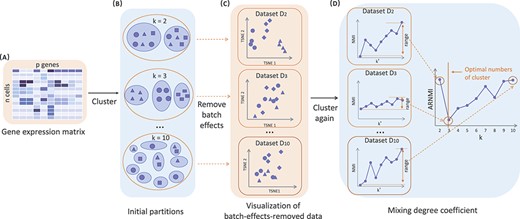
The workflow of REBET. (A). Inputs of this method: a gene expression data matrix of |$n$| cells in rows and |$p$| genes in columns. (B). SC3 was used to cluster the input data with a range of potential cluster numbers (From top to bottom, |$k $| from 2 to 10). Small squares, triangles and circles all represent cells, and different shapes indicate different cell clusters (there are three cell clusters in total). When the cells are in the same blue background color circle, it means they are partitioned into the same cluster. (C). Each clustering result was treated as a batch variable to remove the batch effect from the input data. To illustrate the effect of removing batch effects, we visualized the batch-effect-removed data by applying t-distributed Stochastic Neighbor Embedding(t-SNE) for dimensionality reduction. When the |$k $| value is less than the true number of cell clusters, the batch-effect-removed data |$\textbf{D}_{k}$| still contains the information of the cell cluster label. Such as Dataset |$\textbf{D}_{2}$| can still be separated by the first principal component. (D). The batch-effect-removed data were clustered separately again, and the mixing degree coefficient, ARNMI, was calculated. The number of clusters corresponding to the minimum ARNMI value is the number of cell clusters determined by REBET.
Generation of initial clusters
We first applied median centralization to gene expression data. We partition the cells using all possible numbers of clusters |$ k\in [2,K] $|. Then for each k, we can obtain labels |$\textbf{y}_{k}$| for each of the cells being clustered, and |$\textbf{y}_{k}$| is a vector of the resulting integers indicating the cluster to which each cell is allocated.
For each possible number of clusters k, each cell will be allocated a label. After the first step, we generate K-1 initial clusters.
Removal of between-cluster variance
Cells from different clusters can be regarded as cells from different batches, and the batch effect removal is equivalent to eliminating differences between clusters. Therefore, in the second step, we treat each |$\textbf{y}_{k}$| as a batch variable, and remove the batch effects from the input data D to obtain K-1 datasets |$ \lbrace \textbf{D}_{2},...,\textbf{D}_{K}\rbrace $|. We specify |$\textbf{y}_{k}$| as the known batch variable and remove batch effects using the ComBat function in the R package sva.
ComBat assumes that for gene |$j$|, the sample |$i$| of batch |$b$| follows the following model: |$D_{bij}=\alpha _{j}+Y_{bi} \beta _{b}+\gamma _{jb}+\delta _{jb} \varepsilon _{bij}$|, where |$\alpha _{j}$| is the overall gene expression, |$Y_{bi}$| is a design matrix for sample conditions (In our case, it is |$\textbf{y}_{k}$|), and |$ \beta _{b}$| is the vector of regression coefficients corresponding to |$Y_{bi}$|. |$\gamma _{jb}$| and |$\delta _{jb}$| represent additive and multiplicative batch effects of batch |$b$| on the gene |$j$|, affecting the mean and variance of gene expression in batch |$b$|, respectively. The error terms |$\varepsilon _{bij}$| are assumed to follow a normal distribution with an expected value of zero and the variance of |$ \sigma _{b}^2$|. ComBat then uses the empirical Bayesian method to estimate the parameters [32, 34].
We assume that cells from different clusters are evenly mixed after batch effect is removed if and only if k corresponds to a true number of clusters of |$k_t$|. We then identified the number of cell clusters by evaluating the mixed uniformity of batch-effect-removed data |$\textbf{D}_{k}$|. The closer |$k$| is to the true number of cell clusters |$k_t$|, the more thoroughly the between-cluster variance is removed. The batch-effect-removed data will allow the cells of different clusters to mix more uniformly.
Identifying the number of cell types based on clustering of batch-effect-removed data
Datasets
Simulated data
To demonstrate that REBET can find the number of clusters, we used the Splatter package to simulate scRNA-seq data with known cluster information [36]. In Splatter, the dispersion between clusters is determined by two parameters, de.prob and de.facLoc. De.prob represents the probability of a gene being selected as a differentially expressed gene, and de.facLoc represents the expression level of differentially expressed genes. A higher de.prob means that more genes are differentially expressed, but changing de.facLoc would change the differentially expressed level of the same number of genes. The larger the values of de.prob and de.facLoc, the greater the difference between clusters. We set the parameters de.prob and de.facLoc to 0.1 and 0.2, respectively to generate four different parameter settings, which were denoted as Exp1, Exp2, Exp3and Exp4 (Table 1). Each parameter setting generated eight datasets, and the number of their clusters ranged from 2 to 9 (Supplementary Tables S1–S4). Each dataset has 200 cells, with each cell measured on 10 000 genes. The probability of cells being divided into each cluster was the same.
The performance of SC3-TW, CC, PINS, SNF, Seurat, SIMLR, ROGUE and REBET in determining the number of cell clusters of simulated datasets with different dispersion between clusters. Eight datasets were simulated for each parameter setting*
| Parameters | Number of datasets accurately estimated | |||||||||
|---|---|---|---|---|---|---|---|---|---|---|
| de. prob | de. facLoc | SC3- TW | CC | PINS | SNF | Seurat | SIMLR | ROGUE | REBET | |
| Exp1 | 0.1 | 0.1 | 0 | 1 | 0 | 1 | 5 | 1 | 3 | 4 |
| Exp2 | 0.2 | 0.1 | 1 | 4 | 0 | 1 | 4 | 3 | 4 | 8 |
| Exp3 | 0.1 | 0.2 | 0 | 1 | 0 | 1 | 4 | 0 | 2 | 7 |
| Exp4 | 0.2 | 0.2 | 1 | 5 | 0 | 1 | 6 | 2 | 5 | 6 |
| All | – | – | 2 | 11 | 0 | 4 | 19 | 6 | 14 | 25 |
*The number in bold indicates the maximum number of datasets that accurately estimated.
scRNA-seq data
To test and verify the effectiveness of our method, we applied the REBET and seven other classical subtyping methods to fourteen published scRNA-seq datasets with known cell subtypes [4, 5, 37–50]. All datasets have defined cell type information. For each dataset, we used the expression units and cell types provided by the authors (Table 2). The t-distributed Stochastic Neighbor Embedding (t-SNE) plots of the original gene expression data of Engel dataset and Zhou dataset is shown in Figure 2 and Supplementary Figure S1A, and the t-SNE plots of other datasets are shown in Supplementary Figure S2. The real scRNA-seq datasets can be accessed through the GEO database.
Summary of the 14 real benchmarking datasets
| Datasets | # Cells | # Genes | Units | Organisms | References |
|---|---|---|---|---|---|
| Zhou | 181 | 23624 | FPKM | Mouse | Zhou et al., 2016 [38] |
| Yan | 90 | 20214 | RPKM | Human | Yan et al., 2013 [40] |
| Treutlein | 80 | 23129 | FPKM | Mouse | Treultein et al., 2014 [45] |
| Ramskold | 33 | 21042 | RPKM | Mouse | Ramskold et al., 2012 [5] |
| Patel | 430 | 5948 | TPM | Human | Patel et al., 2014 [44] |
| Leng | 247 | 19080 | TPM | Human | Leng et al., 2015 [48] |
| Grover | 135 | 15158 | RPKM | Mouse | Grover et al., 2016 [43] |
| Goolam | 124 | 40315 | CPM | Mouse | Goolam et al., 2016 [41] |
| Engel | 203 | 23337 | RPM | Mouse | Engel et al., 2014 [46] |
| Deng | 259 | 22147 | RPKM | Mouse | Deng et al., 2014 [42] |
| Chung | 518 | 41821 | TPM | Human | Chung et al., 2017 [4] |
| Biase | 49 | 25384 | FPKM | Mouse | Biase et al., 2014 [39] |
| Usoskin | 622 | 19153 | RPM | Mouse | Usoskin et al., 2015 [50] |
| Cirstea | 1534 | 21785 | TPM | Human | Karaayvaz et al., 2018 [49] |
![REBET illustrated on the Engel dataset (The true number of clusters is 4). (A) The t-SNE plot of the original gene expression data with cells colored according to the true label. (B–E). The scatter plots of batch-effect-removed data $\textbf{D}_{k}$ ($ k\in [2,5] $) with the first dimension reduction component as the x-axis and the second dimension reduction component as the y-axis after t-SNE dimensionality reduction. Cells are colored according to the true label. (B) Batch-effect-removed data still have obvious clusters. (C) The cells of NKT0 subpopulation shown in the lower-left corner and the top still clustered together. (D) All cells are mixed together, containing cells from the NKTO subpopulation and the NTK2 subpopulation. (E) Except for the cells of NTK2 subpopulation, other cell subpopulations are also mixed together. (F) Error bar plot of the mixing degree coefficient ARNMI values in the range $k=2,3,...,9$. When $k$ is between 2 and 4, ARNMI goes down. From (B) to (D), the different subpopulations of cells are also increasingly uniformly mixed together. REBET accurately estimated the number of cell subpopulations.](https://oup.silverchair-cdn.com/oup/backfile/Content_public/Journal/bib/22/6/10.1093_bib_bbab204/1/m_bbab204f2.jpeg?Expires=1750207983&Signature=UySu8YcckkA~uJnD9jeZoB5CoXut-ZcrccOJS85AyTQAUjN4nGm-fdJJltBfSMoxDMtvD1johDJAd9MdwYx43K6ZN6usJcR9nYYXzCaWozh9zdjt1ANKDKuiMFW2i-DO7ass581YztCUsOPFGLj-KaY-gRV8tT4eaNftaPOMrjUDrDooq~k6wjGyDXGyZBknP6l93aCJts8vacdAzR0ehZ6xQMvYRdPUfAUQ276I0MQtq2ujb0bnPkVYTEp~RA~SnOr~9zSoFeuFaeozL31qJUHmhqxCi641O7dWwkiyJcRH7tVGapKJ13T025uqr83N9MKbrHF7vKuVncFfviaUmA__&Key-Pair-Id=APKAIE5G5CRDK6RD3PGA)
REBET illustrated on the Engel dataset (The true number of clusters is 4). (A) The t-SNE plot of the original gene expression data with cells colored according to the true label. (B–E). The scatter plots of batch-effect-removed data |$\textbf{D}_{k}$| (|$ k\in [2,5] $|) with the first dimension reduction component as the x-axis and the second dimension reduction component as the y-axis after t-SNE dimensionality reduction. Cells are colored according to the true label. (B) Batch-effect-removed data still have obvious clusters. (C) The cells of NKT0 subpopulation shown in the lower-left corner and the top still clustered together. (D) All cells are mixed together, containing cells from the NKTO subpopulation and the NTK2 subpopulation. (E) Except for the cells of NTK2 subpopulation, other cell subpopulations are also mixed together. (F) Error bar plot of the mixing degree coefficient ARNMI values in the range |$k=2,3,...,9$|. When |$k$| is between 2 and 4, ARNMI goes down. From (B) to (D), the different subpopulations of cells are also increasingly uniformly mixed together. REBET accurately estimated the number of cell subpopulations.
Data preprocessing
Before applying these methods, we preprocessed the data with reference to SC3, including gene filtering and logarithmic transformation [12]. Gene filters remove genes that are expressed in cells (expression value >2) less than 6%, or those that have a variance of 0. Then logarithmic transformation is performed on the filtered expression matrix after adding pseudo-count 1. To avoid changing the distribution of the data, we do not apply logarithmic transformation when we use the ROGUE method.
Benchmark methods
We applied the SC3, CC, PINS, SNF, Seurat, SIMLR and ROGUE methods to the above twelve published scRNA-seq datasets for evaluation and comparison of determining the number of cell clusters. SC3 is a consensus method that combines multiple clustering solutions. The first step is to use z-score to normalize the input data and record the normalized data as matrix Z. The second step is to calculate the eigenvalue of |$\textbf{Z} ^{\prime }\textbf{Z} $|. The final number of clusters is the number of eigenvalues that are significantly different from the Tracy–Widom distribution at a significance level of 0.001 [12]. To distinguish the cluster number determination from the clustering method SC3, we denote this method for determining the number of clusters as SC3–TW. In the CC method, a proportion of samples and a proportion of features are subsampled from the data to form subsamples. Then, each subsample is clustered and the consensus matrix of each k is calculated. When the area under the curve leveling off and |$ \Delta k$| approaching zero, the corresponding k value is the number of clusters [51]. For PINS, the data are perturbed by adding Gaussian noise, and then a connectivity matrix is constructed based on the original data and perturbed data for each k (|$ k\in [2,K] $|) to calculate the absolute difference. Next, the empirical cumulative distribution functions of the connectivity difference matrices are calculated. It performs the partitioning based on the highest AUC [27]. The main idea of SNF is to construct a sample network and then effectively fuse the patient similarity network representing the full spectrum of the underlying data [26]. SNF determines the number of clusters by using eigengaps based on network connections. SIMLR provides two methods to estimate the number of clusters. The first method is the Eigengap method. It first calculates the eigenvalues of the Laplace matrix and sorts them in descending order (i.e. |$\lambda _{1},\lambda _{2},\cdots ,\lambda _{n}$|). The number of clusters is estimated as |$\max _{i>1}\left (\lambda _{i+1}-\lambda _{i}\right )$| [13]. The second method is Separation Cost, it determines the number of clusters which results in the greatest largest drop in the value of the separation cost [52]. We get most of the same results using Eigengap method and Separation Cost method, so our results below only show the results of Separation Cost method. Seurat first calculates k-nearest neighbors, constructs the SNN graph, and then uses a smart local moving algorithm to identify community structures [14, 53]. ROGUE first uses differential entropy to describe the distribution of gene expression in single-cell data, and then builds an S-E model to describe the relationship between differential entropy and the mean of gene expression. Based on this model, a ROGUE uniform measurement is designed to evaluate the purity of a cell cluster [24]. For ROUGE, we first used SC3 to cluster gene expression data for all possible cluster numbers (|$ k\in [2,K] $|), and then used ROGUE to select the number of cell clusters according to the clustering results.
Evaluation criteria
Accuracy evaluation of the estimated number of cell clusters
For each dataset, we can calculate the deviation between the estimated number of cell clusters and the true number of cell clusters. To compare the accuracy of each method in estimating the number of cell clusters, we use the median of absolute deviations of the 14 datasets as the evaluation index of accuracy.
Evaluation metric for clustering
After determining the number of clusters with REBET, we used SC3 to cluster the gene expression data and denoted it as REBET-SC3. After using SC3-TW, CC, PINS, SNF, Seurat, SIMLR and ROGUE to estimate the number of clusters, we use SC3, CC, PINS, SNF, Seurat, SIMLR and SC3 to cluster the original data. The adjusted Rand index (ARI) is used to calculate the similarity between the clustering results and the known true clusters, which can be used to evaluate the clustering result. If the estimated label is the same as the true label, the ARI is 1, and the ARI decreases with increasing inconsistency [54].
Results
Simulated Datasets
To evaluate the accuracy of our method, we applied REBET and other compared methods to 32 simulation datasets with the different number of clusters and dispersion between clusters.The median of the absolute deviation between the number of cell clusters estimated by REBET, SIMLR and Seurat methods and the true cell clusters is 0 across the 32 simulated datasets (Fig. 3). The deviation of REBET was less variable than other methods (Figure 3). REBET accurately estimated the number of cell clusters in 25 datasets, which was the most accurate estimate among the above methods (Table 1). Followed by Seurat and ROGUE, which accurately estimated 19 and 14 datasets, respectively (Table 1).
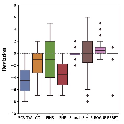
The deviations between the estimated number of cell clusters and the true number of cell clusters for the 32 simulated datasets.
For the datasets in Exp1 with a small dispersion between clusters, REBET accurately estimated the number of clusters in four datasets (Table 1, Supplementary Table S1). Except that Seurat accurately estimated the number of clusters of five datasets, other methods performed worse (Table 1, Supplementary Table S1). REBET accurately estimated the number of clusters in all eight datasets of Exp2. All of the other seven methods performed worse (Table 1, Supplementary Table S2). For all the datasets in Exp3, REBET only incorrectly estimated the dataset with eight clusters (Supplementary Table S3). REBET estimated the number of clusters to 7, and other methods had not accurately estimated (Supplementary Table S3). For the datasets in Exp4 with a large dispersion between clusters, both REBET and Seurat accurately estimated the number of clusters in six datasets (Table 1). The number of clusters in the dataset with the true number of clusters 5 and 6 were estimated by REBET to be 6 and 7 (Supplementary Table S4). This may be because even if the correct batch effect is defined, the removal of the batch effect may be incomplete. The number of clusters determined by REBET is still close to the true number of clusters. No matter what the true number of clusters |$k$| is, REBET can robustly determine the number of clusters in the majority datasets.
We use the simulated dataset with a true number of clusters of 3 in Exp2 to illustrates how REBET determines the number of clusters (Figure 4). As mentioned above, the input data were first partitioned into k classes. In the second step, for each k (|$ k\in [2, K] $|), we removed the differences between different clusters by treating the cluster label as a batch variable and then removing the effect of this batch variable. When k is equal to the true number of clusters, the batch-effect-removed data for each true cluster should be mixed uniformly. To explain more clearly, we applied t-SNE to the batch-effect-removed data |$\textbf{D}_{k}$|. Figure 4B- 4D show the t-SNE plots for the batch-effect-removed data |$\textbf{D}_{k}$| with cells colored according to the true label for |$k=2$|, |$k=3$| and |$k=4$|. When |$k=2$|, we can see that the first dimension component can divide the cells into three classes, indicating that the batch-effect-removed data |$\textbf{D}_{2}$| still contains information of the label. When |$k>2$|, no clear cluster is seen based on the dimension reduction components. When |$k$| is the true number of clusters 3, the average range of normalized mutual information (ARNMI) reaches its minimum (Figure 4E). The result shows that REBET can correctly estimate the true clusters of this dataset.
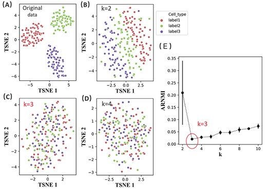
The REBET algorithm applied on the simulated dataset with a true number of clusters of 3 in Exp2. The dataset consists of 200 samples and 10 000 genes. Each of the second and third classes has 65 samples whereas the first class has 70 samples (a total of 200 samples). (A) The t-SNE plot of the original gene expression data with cells colored according to the true label. (B–D) The t-SNE plots of the batch-effect-removed data |$ \textbf{D}_{k}$| with cells colored according to the true label for |$k=2$|, |$k=3$| and |$k=4$|. (E) Error bar plot of the ARNMI values for the dataset. REBET correctly estimated the true number of clusters.
For the 32 simulated datasets, we found that the ARI of REBET-SC3 of 25 datasets was the highest or the same as the ARI obtained by the other seven methods (Supplementary Figure S3). Table 3 shows the median ARI for the simulation datasets under the same parameter settings. The method with the highest ARI in each row is in boldface. We find that REBET can improve the clustering performance (Table 3).
The median ARI values for SC3, CC, PINS, SNF, Seurat, SIMLR, ROGUE-SC3 and REBET-SC3 of simulated datasets with different dispersion between clusters. Eight datasets were simulated for each parameter setting*
| Parameters | Median ARI | |||||||||
|---|---|---|---|---|---|---|---|---|---|---|
| de. prob | de. facLoc | SC3 | CC | PINS | SNF | Seurat | SIMLR | ROGUE -SC3 | REBET -SC3 | |
| Exp1 | 0.1 | 0.1 | 0 | 0 | 0 | 0 | 0.85 | 0.19 | 0.96 | 0.92 |
| Exp2 | 0.2 | 0.1 | 0 | 0.99 | 0.43 | 0.01 | 0.95 | 0.75 | 0.95 | 1 |
| Exp3 | 0.1 | 0.2 | 0 | 0 | 0 | 0 | 0.89 | 0.39 | 0.92 | 1 |
| Exp4 | 0.2 | 0.2 | 0 | 1 | 0.47 | 0.01 | 0.99 | 0.73 | 1 | 1 |
*The method with the highest ARI in each row is in boldface.
We changed the method of removing batch effect in the second step to limma [31]. We found that the number of clusters can be estimated accurately on the majority of datasets. It accurately estimated the number of clusters for the five datasets of Exp1. For the datasets in Exp2 and Exp3, the number of clusters of seven datasets can be accurately estimated. It accurately estimated the number of clusters for all eight datasets in Exp4 (Supplementary Table S5).
scRNA-seq Datasets
We applied REBET and the other seven methods to 14 scRNA-seq datasets. By default, we set the maximum number of cell clusters K to 10. As shown in Table 4, the absolute deviation between the true number of clusters and the number of clusters estimated by REBET was less than or equal to 2 for all datasets except the Patel and Deng datasets. The estimated number of clusters for the eight datasets (Yan, Grover, Biase, Ramskold, Patel, Engel, Leng and Usoskin) were the same as the true number of clusters, whereas the deviation of the Cristea dataset was only one. For the Chung, Treutlein and Goolam datasets, the number of cell clusters estimated by REBET differed from the true number of cell clusters by 2. Furthermore, the number of cell clusters estimated by REBET were still closest to the true number of cell clusters in the Deng and Chung datasets.
The performance of SC3-TW, CC, PINS, SNF, Seurat, SIMLR, ROGUE and REBET in determining the number of cell clusters from scRNA-seq data*
| Datasets | # True clusters | Estimated number of cell clusters | |||||||
|---|---|---|---|---|---|---|---|---|---|
| SC3-TW | CC | PINS | SNF | Seurat | SIMLR | ROGUE | REBET | ||
| Zhou | 8 | 6 | 10 | 3 | 2 | 4 | 6 | 4 | 2 |
| Yan | 6 | 4 | 2 | 2 | 2 | 3 | 2 | 4 | 6 |
| Treutlein | 5 | 4 | 10 | 2 | 3 | 2 | 4 | NA | 3 |
| Ramskold | 7 | 3 | 2 | 2 | 4 | 1 | 4 | 2 | 7 |
| Patel | 5 | 17 | 7 | 7 | 2 | 6 | 4 | 2 | 5 |
| Leng | 3 | 2 | 3 | 2 | 3 | 4 | 2 | 4 | 3 |
| Grover | 2 | 3 | 2 | 3 | 2 | 4 | 3 | 2 | 2 |
| Goolam | 5 | 3 | 2 | 3 | 4 | 4 | 4 | 6 | 7 |
| Engel | 4 | 3 | 3 | 2 | 2 | 5 | 4 | NA | 4 |
| Deng | 10 | 6 | 2 | 3 | 2 | 7 | 3 | 6 | 7 |
| Chung | 4 | 15 | 9 | 2 | 2 | 11 | 1 | 9 | 2 |
| Biase | 3 | 3 | 2 | 3 | 2 | 2 | 6 | 2 | 3 |
| Usoskin | 4 | 9 | 2 | 7 | 2 | 7 | 3 | 10 | 4 |
| Cristea | 6 | 39 | 3 | 4 | 2 | 13 | 9 | 8 | 7 |
*For each dataset, the numbers highlighted in bold are the most accurate estimates of the number of cell clusters. ROGUE produced errors for Treutlein and Engel datasets, shown as an NA value.
The cell clusters are treated as batches, and we assumed that when the number of clusters is the same as the number of batches, the batch effect is removed from the original gene expression data, and the cells from different subpopulations will mix most uniformly. To illustrate the effect of removing batch effects, we applied t-SNE to reduce the dimensionality of batch-effect-removed data. Here, we take the Engel dataset as an example. First, the Engel dataset was clustered into k classes (|$ k\in [2,10] $|) and the clustering labels were recorded as |$\textbf{y}_{k}$|. Then we used |$\textbf{y}_{k}$| as the batch variable to remove the batch effect from the input data for the Engel dataset and obtained the batch-effect-removed data |$\textbf{D}_{k}$|. We visualized the batch-effect-removed data |$\textbf{D}_{k}$| with t-SNE (Figure 2B–2E). Cells are colored according to the true label. There are obvious clusters in data |$\textbf{D}_{2}$| (Figure 2B). As |$k$| goes from 2 to 4, the cells from different subpopulations are increasingly uniformly mixed together (Fig. 2B–2D). And ARNMI goes down (Figure 2F). When |$k=3$|, the cells of the NKT0 subpopulation shown in the lower-left corner and the top still clustered together (Figure 2C). When |$k=5$|, the cells from different subpopulations are mixed except for the cells from the NTK2 subpopulation with the color purple (Figure 2E). This is because |$k$| is larger than the true number of cell subpopulations, and the cells of the NTK2 subpopulation are initially partitioned into two clusters. Although the NTK2 subpopulation and NTK0 subpopulation are mixed in each cell subpopulation in Figure 2D. These findings validated our assumptions. Our proposed mixing degree coefficient ARNMI is minimum when |$k$| is equal to 4 (Figure 2F). Therefore, REBET accurately estimated that the number of cell subpopulations of the Engel dataset was 4.
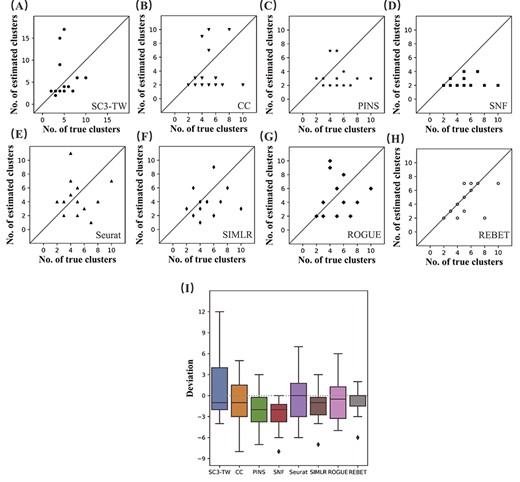
Accuracy of the estimated number of cell clusters. (A–H) Correlations between the cluster numbers estimated by SC3-TW, CC, PINS, SNF, Seurat, SIMLR, ROGUE and REBET and the true cluster numbers, for the 14 benchmarking datasets. (I) The deviations between the estimated number of cell clusters and the true number of cell clusters. The median absolute deviation for the estimate by REBET of the number of cell clusters is the smallest of the eight methods.
We compared our method with other methods in terms of the accuracy of the number of clusters estimation and the clustering results. We first compared the accuracy of the estimated number of cell clusters. Table 4 shows the performance of the SC3-TW, CC, PINS, SNF, Seurat, SIMLR, ROGUE and REBET methods in determining the number of cell clusters based on the gene expression data. The numbers highlighted in bold are the most accurate estimates of the number of cell clusters (The estimated number of cell clusters is the closest to the true number of cell clusters) in their respective rows. As shown in Table 4, REBET performed robustly across various datasets in estimating the number of cell clusters. For the 14 datasets, the number of cell clusters estimated by the REBET in 11 datasets was the most accurate. SNF and SIMLR made the most accurate estimation for four datasets, whereas SC3-TW only made the most accurate estimation for three datasets. To view the accuracy of the estimation by each method of the number of clusters more clearly, we drew a scatter plot with the number of clusters estimated by each method as the y-axis and the true number of clusters as the x-axis (Figure 5). SC3-TW, PINS and SNF tend to underestimate the number of clusters (Figure 5). For the fourteen datasets, the median absolute deviation of the number of cell clusters estimated by REBET was 0, which was the smallest among the eight methods (Figure 5I). And the variance of REBET was smaller. In short, REBET outperformed existing solutions according to the median absolute deviation.
For the outlier of REBET in Figure 5I, REBET incorrectly estimated the number of clusters of the Zhou dataset as 2 (Table 4). No matter what |$k$| is, after removing batch effect, the cells of different clusters do not mix, especially the cells colored by yellow (Supplementary Figure S1). The reason why REBET incorrectly estimated the number of clusters of the Zhou dataset may be that the initial partition obtained by clustering was not accurate enough, or that the batch effect is complex so that it can not be captured by ComBat.
Figure 6 shows the final clustering result evaluation index ARI of each method for the fourteen datasets. REBET-SC3 performed better than all of the other seven methods for eight datasets: Usoskin, Biase, Deng, Engel, Grover, Leng, Patel and Ramskold (Supplementary Table S6). Furthermore, REBET-SC3 performed better than at least five methods for the other two datasets (Yan and Treutlein) (Figure 6). Then, we observed that the ARI values of REBET-SC3 were higher than that of the original SC3, except for the Cristea, Yan, Treutlein, Goolam, Chung and Zhou datasets. For the Yan dataset, although the original SC3 had a higher ARI than REBET-SC3, REBET accurately estimated the number of cell clusters. The mean and median ARI of REBET-SC3 were both the highest among the compared methods (Figure 6).
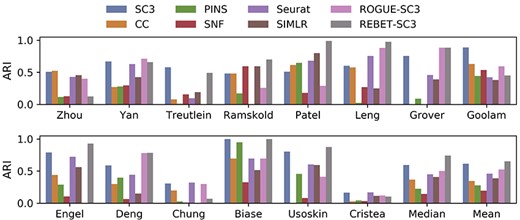
Comparison of clustering performances of SC3, CC, PINS, SNF, Seurat, SIMLR, ROGUE-SC3 and REBET-SC3, measured by Adjusted Rand Index (ARI). ARI is employed to measure the consistency between cluster labels and true labels. The labels “Median” and “Mean” represent the median and mean values across all 14 datasets. The exact ARI values of the 14 datasets are shown in Supplementary Table S6.
Robustness
To test the robustness of REBET, we randomly selected 95% of the cells from each cluster in each dataset and reran the REBET and the other methods 10 times [55]. We found that REBET estimated a relatively stable and accurate number of cell clusters. For the 32 simulated datasets, there are 25 datasets in which the median absolute deviation between the true number of clusters and the number of clusters estimated by REBET is 0 (Figure 7). For the remaining seven datasets, the median absolute deviation of REBET for 5 datasets is still the smallest among the eight methods. When the median absolute deviation of the number of clusters estimated by REBET is 0, the variance of the number of clusters estimated by REBET is also close to 0 (Figure 7).
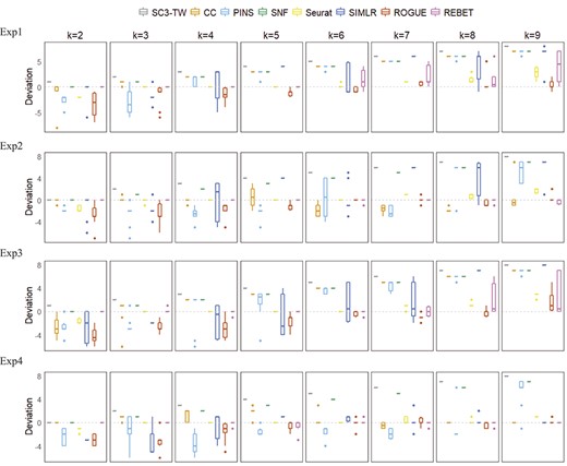
Accuracy and robustness of the estimated number of cell clusters in the simulated datasets. Panels are box plots of the deviation between the true number of cell clusters and the estimated number of cell numbers for the 32 simulated datasets, across 10 times of randomly sampling 95% of cells. Panels in the same row indicate the same separation parameter setting between clusters (Exp1, Exp2, Exp3 and Exp4), and panels in the same column indicate the true number of cell clusters |$k$|.
For the 14 real scRNA-seq datasets, the median absolute deviation of the estimated number of clusters of REBET after 10 samplings is the minimum on the 8 datasets (Yan, Ramskold, Patel, Grover, Chung, Biase, Usoskin and Cristea) (Figure 8, Supplementary Table S7). Especially for Yan, Ramskold, Patel, Usoskin and Cristea datasets, REBET performed best in terms of robustness and accuracy (Figure 8). For the Grover dataset, REBET, ROGUE and SNF accurately estimated the number of cell clusters each time (Figure 8).
Discussion
In this study we proposed a new method, REBET, to estimate the number of clusters of cells based on clustering of batch-effect-removed data. We treated different clusters as different batches, and then removed the batch effects, that is, the between-cluster variance was removed. When the number of cell clusters is correctly estimated and the clustering result is treated as a batch variable, the batch effect can be completely removed. From the scatter plot of t-SNE dimensionality reduction for batch-effect-removed data, it can be seen that the data will not have obvious clustering and will be evenly mixed. The optimal number of clusters can be achieved by minimizing the mixed degree coefficient that we defined. The source codes for the REBET are freely available at https://github.com/genemine/REBET.
Determining the number of cell clusters is the main challenge in scRNA-seq data analysis. Whereas, both simulation studies and real data applications indicated that REBET can accurately estimate the number of cell clusters in the majority of data. We generated four sets of simulated datasets, each consisting of eight datasets. The median absolute deviation of the number of cell clusters estimated by REBET was 0. REBET accurately estimated the number of cell clusters in 25 datasets, and the estimated deviations for the other six datasets were small. No matter what the true number of clusters |$k$| is, REBET can robustly determine the number of clusters in the majority of data.
We also benchmarked REBET along with other seven subtyping methods (SC3-TW, CC, SNF, PINS, SIMLR, Seruat and ROGUE) for 14 published scRNA-Seq datasets. REBET achieves consistently satisfactory performance in the majority of datasets. The median deviation of the number of cell clusters estimated by REBET was 0, and the variance was the smallest among the eight methods. The resampling experiment evaluated the robustness of REBET in determining the number of clusters. We found that REBET estimated a relatively robust and accurate number of clusters. After determining the number of clusters with REBET, we used SC3 to cluster the gene expression data. The results of this study show that REBET can improve the clustering performance.
We tested whether our method can correctly estimate the number of clusters for data with batch effect. We generated eight simulation datasets with the true number of cell clusters ranging from 2 to 9. The cells of each cluster of these eight datasets are from 2 batches (Supplementary Figure S4). We first used ComBat to remove batch effects from the original data, and then use REBET to estimate the number of cell clusters. REBET accurately estimated the number of clusters in the all datasets (Supplementary Figure S5). For data with batch effect, we suggest removing batch effects before applying REBET.
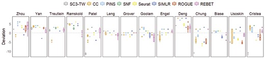
Accuracy and robustness of the estimated number of cell clusters. Panels are box plots of the deviation between the true number of cell clusters and the estimated number of cell numbers for the 14 real datasets, across 10 times of randomly sampling 95% of cells.
REBET does not have any other parameters (except for the maximum number of clusters K). REBET relies on methods to remove batch effects and clustering methods. By default, the clustering method we choose is SC3, and the method used for removing batch effects is Combat. We can also use the limma method to remove batch effects (Supplementary Table S5). The eight methods consume almost the same memory. For example, when the number of cells is 200, the running time is about 30 minutes (Supplementary Table S8). However, other methods (SC3-TW, CC, Seurat, SIMLR and PINS) are as fast as a few seconds, and ROGUE only takes a few minutes (Supplementary Table S8). The SC3 method does not run fast, and SC3 needs to be run multiple times in REBET. So REBET is time-consuming.
With the explosive growth of scRNA-seq data, efficient analysis methods are demanding. The determination of the number of cell clusters is fundamental to scRNA-seq analysis [55]. REBET can accurately and robustly estimate the number of cell clusters, which will facilitate further analysis of scRNA-seq data. Indeed, there are still some topics that can be further expanded. First, we can improve the method to remove the batch effect, to remove the batch effect better. Second, we can select genes that accurately contain the information of cell clusters, which will contribute to more accurate initial partitioning and more thorough removal of batch effects. Thirdly, we can analyze the difference of isoform between different clusters, so we can consider adding isoform information when determining the number of cell clusters.
Understanding the development of an organ requires characteristic cell subpopulations, so it is important to quantify single-cell subpopulations accurately. Motivated by the practice of batch effect removal, we considered cell clusters as batches. We developed REBET (REmoving Batch Effect and Testing), a new method for determining the number of cell clusters based on single-cell RNA-seq (scRNA-seq) data.
The performances of REBET and other seven state-of-the-art methods are compared on simulated datasets with different number of clusters and dispersion between clusters. No matter what the true number of clusters is, REBET can robustly determine the number of clusters in the majority of data.
The performances of REBET and other seven state-of-the-art methods are compared on 14 published scRNA-seq datasets. REBET can accurately and robustly estimate the number of cell clusters and outperform existing methods. By comparing the clustering evaluation metric adjusted Rand index (ARI), we find that REBET can improve the clustering performance.
Funding
This work is supported by National Natural Science Foundation of China (61972185, U1909208), 111 Project (No. B18059) and Hunan Provincial Science and Technology Program (2018WK4001).
Zhao-Yu Fang is a graduate student at the School of Mathematics and Statistics, Central South University, Hunan, China. Her research interests include bioinformatics and machine learning.
Cui-Xiang Lin is a graduate student in the Hunan Provincial Key Lab on Bioinformatics, School of Computer Science and Engineering at Central South University, Hunan, China. Her research interests include bioinformatics and systems biology.
Yun-Pei Xu is a graduate student in the Hunan Provincial Key Lab on Bioinformatics, School of Computer Science and Engineering at Central South University, Hunan, China. His research interests include single-cell RNA-seq data analysis and machine learning.
Hong-Dong Li is an associate professor in the Hunan Provincial Key Lab on Bioinformatics, School of Computer Science and Engineering at Central South University, Hunan, China. His research interests include alternative splicing, computational medicine and systems biology.
Qing-Song Xu is a professor at the School of Mathematics and Statistics, Central South University, Hunan, China. His research interests include bioinformatics, computational medicine and chemometrics.
References
