A survey on predicting microbe-disease associations: biological data and computational methods

Wen, Zhongqi; Yan, Cheng; Duan, Guihua; Li, Suning; Wu, Fang-Xiang; Wang, Jianxin

doi:10.1093/bib/bbaa157

Abstract

Various microbes have proved to be closely related to the pathogenesis of human diseases. While many computational methods for predicting human microbe-disease associations (MDAs) have been developed, few systematic reviews on these methods have been reported. In this study, we provide a comprehensive overview of the existing methods. Firstly, we introduce the data used in existing MDA prediction methods. Secondly, we classify those methods into different categories by their nature and describe their algorithms and strategies in detail. Next, experimental evaluations are conducted on representative methods using different similarity data and calculation methods to compare their prediction performances. Based on the principles of computational methods and experimental results, we discuss the advantages and disadvantages of those methods and propose suggestions for the improvement of prediction performances. Considering the problems of the MDA prediction at present stage, we discuss future work from three perspectives including data, methods and formulations at the end.

microbe-disease prediction, microbe/disease similarity, similarity calculation method, cross validation

Introduction

Microbial communities, which are composed of bacteria, archaea, fungi, viruses and protozoa [1], ubiquitously colonize in the human body. Microorganisms are usually beneficial to human beings. For instance, probiotics in guts are good for fermenting undigested carbohydrates so as to manufacture nutrition which is needed by the human beings [2, 3]. They also make great contributions to the maturity of the immune system [4, 5]. In addition, microbial communities are essential to guarantee that the homeostasis of extracellular fluid and intracellular environment are stable [6]. Hydrogen peroxide and lactic acid, the product of the vaginal Lactobacillus species, protect female vaginas from invasion of pathogens [7, 8]. The microbiota is also able to activate the repair process of the damaged physiological functions as well, such as fixing the intestinal epithelium through the MyD88-dependent process [9].

A group of balanced microorganisms keep the human body away from physiological disorders, while the unusual growth or decline of microorganism population is possibly related to the occurrence of disease. More clinical trials and advanced sequencing technologies make it possible to study intricate microbe-disease associations (MDAs) [10, 11]. For example, infections of facial follicles are typically caused by the massive reproduction of Staphylococcus aureus [12]. It is also known that many regions inside the human body are suitable habitats for various microorganisms, such as the oral cavity. Several studies have implicated that changes in the composition of oral microbiota contribute to periodontitis [13, 14]. The gut microbiota is greatly involved in host metabolic and immunomodulatory activities, forming the most complex microecosystem in human body. Abnormal host–gut microbiota interactions greatly affect host physical health and possibly lead to diseases. For example, the dysbiosis of gut microbiome is a prominent contributor to the chronic inflammation in inflammatory bowel disease [15] and hypertension [16] patients. The colonic mucosa is cumulatively exposed to diet-induced microbial carcinogenic metabolites, promoting colorectal cancer [17]. With regard to obesity that has been proved to correlate with the gut microbiota, a strategy for identifying the pathogenic agent in the gut microbiota has been already proposed, combining with a spectrum of microbiome-wide association studies [18].

As mentioned previously, studies on pathomicrobiology open up promising perspectives. Some small-scale databases focusing on genomic information of specific microbes have been established [19, 20]. Other comprehensive microbial databases such as SILVA [21], IMG/M [22], Pfam [23], M3D [24], MiST [25] and TCDB [26], covering diverse branches of microbiology (e.g. genome, metagenome, proteome, transcription and metabolism), have also been created. Meanwhile, some researchers develop and adopt computational methods to detect microbial influences on human diseases. For example, Coelho et al. have proposed a computational method to predict the impact of microbial proteins on human biological events, which takes the relationship between microbial and human proteins into consideration [27]. Another famous instance related to the microbe project is the Human Microbiome Project launched in 2007 [28].

Discovering MDAs would be truly useful in disease-related areas (e.g. pathogenic genes and drugs) [29]. Taking drug repositioning as an example, type 2 diabetes shares a high similarity with colorectal carcinoma based on their associations with microbes, which infers that these two diseases could be treated with the same drug. This hypothesis has been tested and verified [30, 31]. Moreover, discoveries of MDAs provide plenty of perspectives on disease mechanisms. Accurate prediction of associations narrows down the MDA potential search space, which reduces the time, effort and cost of wet labs’ projects. Figure 1 depicts an entire process that includes data collection, computational prediction, clinical validation and pathology inference.

Figure 1

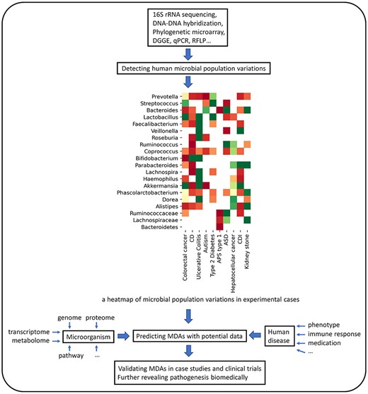
Three main procedures of exploring the relationship between microbes and diseases: (i) Differences between the diseased group and healthy group in microbial populations are captured from metagenome samples based on sequencing technologies. Researchers normalize quantitative differences from reported cases and curate the MDA dataset. (ii) High-confidence MDAs are derived by the computational prediction based on the MDA dataset, microbe-centric data and disease-centric data. (iii) Biologists screen the candidates and seek biomedical interpretation.

Open in new tab Download slide

However, there is no overarching survey so far regarding the MDA prediction. Therefore, we try to comprehensively review computational methods for the MDA prediction in this study. We divide the computational methods into five categories [32, 33] as shown in Table 1. The following itemized list briefly describes their nature:

Path-based methods: In heterogeneous networks, path-based methods make the prediction by computing path-based scores between microbe nodes and disease nodes.
Random Walk methods: A walker randomly walks in the transition probability network consisting of microbe and disease nodes. These methods search for a potential association by measuring the probability of a random walker that has completed a path starting a node from a side of the association and ending a node from another side.
Bipartite local models (BLMs): BLMs compute the prediction scores of MDAs from two perspectives: diseases and microbes. Prediction scores of both sides are integrated, which is regarded as final prediction score.
Matrix factorization methods: An association matrix is factorized into two low-dimensional matrices where one represents features of diseases while another represents features of microbes. The product of two low-dimensional matrices is the final predicted matrix.
Other methods: Some methods could not be classified into the above-mentioned categories, and thus these methods are grouped into ‘other methods’.

Table 1

Open in new tab

Different methods to predict MDAs in each category

Category	Method	Description
Path-based methods	KATZHMDA [40], PBHMDA [63], MDPH_HMDA [40], BWNMHMDA [60],WMGHMDA [47]	Path-based methods generally take into account numbers and weighted scores of various types of paths between two nodes.
Random walk methods	RWRH [51], BiRWHMDA [58], PRWHMDA [49], NTSHMDA [65], BDSILP [53], BiRWMP [69], BRWMDA [68], NBLPIHMDA [67], RWHMDA [66]	Random walk methods construct graph-based transition probability matrix for iterative walking.
BLMs	LRLSHMDA [72], NGRHMDA [70], Wang et al. [36], NCPHMDA [71], KATZBNRA [57]	BLMs perform independent predictions from both microbe and disease sides.
Matrix factorization methods	CMFHMDA [80], GRNMFHMDA [59], NMFMDA [56], KBMF [84], MDLPHMDA [82], mHMDA [86]	Matrix factorization methods optimize two latent informative matrices, whose multiplication approximates the association matrix with different constraint terms.
Other methods	ABHMDA [87], BMCMDA [88], MCHMDA [89]	These methods mainly include ensemble learning and matrix completion.

Category	Method	Description
Path-based methods	KATZHMDA [40], PBHMDA [63], MDPH_HMDA [40], BWNMHMDA [60],WMGHMDA [47]	Path-based methods generally take into account numbers and weighted scores of various types of paths between two nodes.
Random walk methods	RWRH [51], BiRWHMDA [58], PRWHMDA [49], NTSHMDA [65], BDSILP [53], BiRWMP [69], BRWMDA [68], NBLPIHMDA [67], RWHMDA [66]	Random walk methods construct graph-based transition probability matrix for iterative walking.
BLMs	LRLSHMDA [72], NGRHMDA [70], Wang et al. [36], NCPHMDA [71], KATZBNRA [57]	BLMs perform independent predictions from both microbe and disease sides.
Matrix factorization methods	CMFHMDA [80], GRNMFHMDA [59], NMFMDA [56], KBMF [84], MDLPHMDA [82], mHMDA [86]	Matrix factorization methods optimize two latent informative matrices, whose multiplication approximates the association matrix with different constraint terms.
Other methods	ABHMDA [87], BMCMDA [88], MCHMDA [89]	These methods mainly include ensemble learning and matrix completion.

Table 1

Open in new tab

Different methods to predict MDAs in each category

Category	Method	Description
Path-based methods	KATZHMDA [40], PBHMDA [63], MDPH_HMDA [40], BWNMHMDA [60],WMGHMDA [47]	Path-based methods generally take into account numbers and weighted scores of various types of paths between two nodes.
Random walk methods	RWRH [51], BiRWHMDA [58], PRWHMDA [49], NTSHMDA [65], BDSILP [53], BiRWMP [69], BRWMDA [68], NBLPIHMDA [67], RWHMDA [66]	Random walk methods construct graph-based transition probability matrix for iterative walking.
BLMs	LRLSHMDA [72], NGRHMDA [70], Wang et al. [36], NCPHMDA [71], KATZBNRA [57]	BLMs perform independent predictions from both microbe and disease sides.
Matrix factorization methods	CMFHMDA [80], GRNMFHMDA [59], NMFMDA [56], KBMF [84], MDLPHMDA [82], mHMDA [86]	Matrix factorization methods optimize two latent informative matrices, whose multiplication approximates the association matrix with different constraint terms.
Other methods	ABHMDA [87], BMCMDA [88], MCHMDA [89]	These methods mainly include ensemble learning and matrix completion.

Category	Method	Description
Path-based methods	KATZHMDA [40], PBHMDA [63], MDPH_HMDA [40], BWNMHMDA [60],WMGHMDA [47]	Path-based methods generally take into account numbers and weighted scores of various types of paths between two nodes.
Random walk methods	RWRH [51], BiRWHMDA [58], PRWHMDA [49], NTSHMDA [65], BDSILP [53], BiRWMP [69], BRWMDA [68], NBLPIHMDA [67], RWHMDA [66]	Random walk methods construct graph-based transition probability matrix for iterative walking.
BLMs	LRLSHMDA [72], NGRHMDA [70], Wang et al. [36], NCPHMDA [71], KATZBNRA [57]	BLMs perform independent predictions from both microbe and disease sides.
Matrix factorization methods	CMFHMDA [80], GRNMFHMDA [59], NMFMDA [56], KBMF [84], MDLPHMDA [82], mHMDA [86]	Matrix factorization methods optimize two latent informative matrices, whose multiplication approximates the association matrix with different constraint terms.
Other methods	ABHMDA [87], BMCMDA [88], MCHMDA [89]	These methods mainly include ensemble learning and matrix completion.

In following sections, we firstly introduce types of data including MDAs and other data for the similarity calculation. Then similarity calculation methods for MDAs and other data are presented. Next, we describe each prediction method with its classification shown in Table 1. A simplified flowchart of predicting MDAs is shown in Figure 2. After that, we evaluate the methods by comparing prediction performances. Finally, we make recommendations for future work of the MDA prediction.

Figure 2

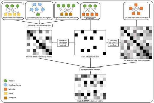
A typical working pattern of computational MDA prediction methods.

Open in new tab Download slide

Materials

Association and similarity data are usually the inputs of computational methods. There are two types of similarity data. One is computed based on original MDAs, and the other is computed based on other data. A description of all raw data used in the MDA prediction is shown in Table 2.

Table 2

Open in new tab

A description of all data used in the MDA prediction

Data	Source	Original form	Size/coverage in HMDAD	Similarity process
MDA data [29]	HMDAD contains evidence of the perturbation of microorganism populations associated with diseases from PubMed (http://www.cuilab.cn/hmdad).	483 deregulatory (increase/decrease) evidence of 292 microbes associated with 39 diseases from published studies	292 microbes mainly at genus and species level, 39 diseases	They are simplified as 450 de-duplicated known MDAs and then used for GIP kernel, Cosine and Spearman correlation similarity calculation.
Gene-based disease data [34, 35]	DisGeNET contains GDAs from UNIPROT, CGI, ClinGen, Genomics England, CTD (human subset), PsyGeNET, Orphanet and those obtained by text mining MEDLINE abstracts (https://www.disgenet.org).	628 685 GDAs, covering GDA scores, diseases specificity index for genes, PMID evidence and so on, between 17 549 genes and 24 166 diseases	37 mapped diseases, 1850 genes, 2715 GDAs	Neighbor-based similarity method uses GDA scores to calculate supplementary similarities among a subset of diseases.
Symptom-based disease data [37, 38]	HSDN integrates large-scale medical bibliographic records of disease–symptom relationships from PubMed (https://www.nature.com/articles/ncomms5212).	Counts and TF-IDF weighted values of co-occurrence between 322 symptoms and 4442 diseases, including 147 978 connections	22 mapped diseases, 269 symptoms, 1858 symptom-disease connections	TF-IDFs of co-occurrence between one disease and all symptoms serve to calculate the symptom-based disease similarity.
Semantics-based disease data [41, 42]	The National Library of Medicine contains MeSH trees to define diseases hierarchically (https://meshb.nlm.nih.gov/search).	Systematically organized disease categories represented by hierarchy trees	33 mapped diseases	Two disease trees consisting of hierarchical descriptors are used for calculating their DAG-based semantic similarity.
Protein family-based microbe data [44]	STRING database contains protein–protein interactions and protein-related knowledge from many data sources (https://string-db.org).	11 362 951 Species-COG mappings and gene neighbor scores between 62 816 502 pairs of COGs	1391 mapped microbes at species level, gene neighbor scores of 932 370 pairs of COGs	The gene neighbor score defines whether an edge between two COGs exists or not. The ratio of edges across two microorganisms to those within either measures their microbe functional similarity and is averaged for genus level.

Data	Source	Original form	Size/coverage in HMDAD	Similarity process
MDA data [29]	HMDAD contains evidence of the perturbation of microorganism populations associated with diseases from PubMed (http://www.cuilab.cn/hmdad).	483 deregulatory (increase/decrease) evidence of 292 microbes associated with 39 diseases from published studies	292 microbes mainly at genus and species level, 39 diseases	They are simplified as 450 de-duplicated known MDAs and then used for GIP kernel, Cosine and Spearman correlation similarity calculation.
Gene-based disease data [34, 35]	DisGeNET contains GDAs from UNIPROT, CGI, ClinGen, Genomics England, CTD (human subset), PsyGeNET, Orphanet and those obtained by text mining MEDLINE abstracts (https://www.disgenet.org).	628 685 GDAs, covering GDA scores, diseases specificity index for genes, PMID evidence and so on, between 17 549 genes and 24 166 diseases	37 mapped diseases, 1850 genes, 2715 GDAs	Neighbor-based similarity method uses GDA scores to calculate supplementary similarities among a subset of diseases.
Symptom-based disease data [37, 38]	HSDN integrates large-scale medical bibliographic records of disease–symptom relationships from PubMed (https://www.nature.com/articles/ncomms5212).	Counts and TF-IDF weighted values of co-occurrence between 322 symptoms and 4442 diseases, including 147 978 connections	22 mapped diseases, 269 symptoms, 1858 symptom-disease connections	TF-IDFs of co-occurrence between one disease and all symptoms serve to calculate the symptom-based disease similarity.
Semantics-based disease data [41, 42]	The National Library of Medicine contains MeSH trees to define diseases hierarchically (https://meshb.nlm.nih.gov/search).	Systematically organized disease categories represented by hierarchy trees	33 mapped diseases	Two disease trees consisting of hierarchical descriptors are used for calculating their DAG-based semantic similarity.
Protein family-based microbe data [44]	STRING database contains protein–protein interactions and protein-related knowledge from many data sources (https://string-db.org).	11 362 951 Species-COG mappings and gene neighbor scores between 62 816 502 pairs of COGs	1391 mapped microbes at species level, gene neighbor scores of 932 370 pairs of COGs	The gene neighbor score defines whether an edge between two COGs exists or not. The ratio of edges across two microorganisms to those within either measures their microbe functional similarity and is averaged for genus level.

Table 2

Open in new tab

A description of all data used in the MDA prediction

Data	Source	Original form	Size/coverage in HMDAD	Similarity process
MDA data [29]	HMDAD contains evidence of the perturbation of microorganism populations associated with diseases from PubMed (http://www.cuilab.cn/hmdad).	483 deregulatory (increase/decrease) evidence of 292 microbes associated with 39 diseases from published studies	292 microbes mainly at genus and species level, 39 diseases	They are simplified as 450 de-duplicated known MDAs and then used for GIP kernel, Cosine and Spearman correlation similarity calculation.
Gene-based disease data [34, 35]	DisGeNET contains GDAs from UNIPROT, CGI, ClinGen, Genomics England, CTD (human subset), PsyGeNET, Orphanet and those obtained by text mining MEDLINE abstracts (https://www.disgenet.org).	628 685 GDAs, covering GDA scores, diseases specificity index for genes, PMID evidence and so on, between 17 549 genes and 24 166 diseases	37 mapped diseases, 1850 genes, 2715 GDAs	Neighbor-based similarity method uses GDA scores to calculate supplementary similarities among a subset of diseases.
Symptom-based disease data [37, 38]	HSDN integrates large-scale medical bibliographic records of disease–symptom relationships from PubMed (https://www.nature.com/articles/ncomms5212).	Counts and TF-IDF weighted values of co-occurrence between 322 symptoms and 4442 diseases, including 147 978 connections	22 mapped diseases, 269 symptoms, 1858 symptom-disease connections	TF-IDFs of co-occurrence between one disease and all symptoms serve to calculate the symptom-based disease similarity.
Semantics-based disease data [41, 42]	The National Library of Medicine contains MeSH trees to define diseases hierarchically (https://meshb.nlm.nih.gov/search).	Systematically organized disease categories represented by hierarchy trees	33 mapped diseases	Two disease trees consisting of hierarchical descriptors are used for calculating their DAG-based semantic similarity.
Protein family-based microbe data [44]	STRING database contains protein–protein interactions and protein-related knowledge from many data sources (https://string-db.org).	11 362 951 Species-COG mappings and gene neighbor scores between 62 816 502 pairs of COGs	1391 mapped microbes at species level, gene neighbor scores of 932 370 pairs of COGs	The gene neighbor score defines whether an edge between two COGs exists or not. The ratio of edges across two microorganisms to those within either measures their microbe functional similarity and is averaged for genus level.

Data	Source	Original form	Size/coverage in HMDAD	Similarity process
MDA data [29]	HMDAD contains evidence of the perturbation of microorganism populations associated with diseases from PubMed (http://www.cuilab.cn/hmdad).	483 deregulatory (increase/decrease) evidence of 292 microbes associated with 39 diseases from published studies	292 microbes mainly at genus and species level, 39 diseases	They are simplified as 450 de-duplicated known MDAs and then used for GIP kernel, Cosine and Spearman correlation similarity calculation.
Gene-based disease data [34, 35]	DisGeNET contains GDAs from UNIPROT, CGI, ClinGen, Genomics England, CTD (human subset), PsyGeNET, Orphanet and those obtained by text mining MEDLINE abstracts (https://www.disgenet.org).	628 685 GDAs, covering GDA scores, diseases specificity index for genes, PMID evidence and so on, between 17 549 genes and 24 166 diseases	37 mapped diseases, 1850 genes, 2715 GDAs	Neighbor-based similarity method uses GDA scores to calculate supplementary similarities among a subset of diseases.
Symptom-based disease data [37, 38]	HSDN integrates large-scale medical bibliographic records of disease–symptom relationships from PubMed (https://www.nature.com/articles/ncomms5212).	Counts and TF-IDF weighted values of co-occurrence between 322 symptoms and 4442 diseases, including 147 978 connections	22 mapped diseases, 269 symptoms, 1858 symptom-disease connections	TF-IDFs of co-occurrence between one disease and all symptoms serve to calculate the symptom-based disease similarity.
Semantics-based disease data [41, 42]	The National Library of Medicine contains MeSH trees to define diseases hierarchically (https://meshb.nlm.nih.gov/search).	Systematically organized disease categories represented by hierarchy trees	33 mapped diseases	Two disease trees consisting of hierarchical descriptors are used for calculating their DAG-based semantic similarity.
Protein family-based microbe data [44]	STRING database contains protein–protein interactions and protein-related knowledge from many data sources (https://string-db.org).	11 362 951 Species-COG mappings and gene neighbor scores between 62 816 502 pairs of COGs	1391 mapped microbes at species level, gene neighbor scores of 932 370 pairs of COGs	The gene neighbor score defines whether an edge between two COGs exists or not. The ratio of edges across two microorganisms to those within either measures their microbe functional similarity and is averaged for genus level.

MDA data

A publicly accessible database, Human Microbe-disease Association Database (HMDAD), provides major data for prediction methods [29]. There are currently hundreds of microorganisms and dozens of diseases sorted out from scraps of published studies in HMDAD by Ma et al. [29]. If there exists a known association between a microbe-disease pair, the corresponding entity in the association matrix is equal to 1, otherwise 0. Furthermore, known associations can be formatted into a bipartite graph that is composed of microbe nodes, disease nodes and edges (associations) connecting them.

Supplementary data for similarity calculation

For the disease similarity:

Gene-based disease data: DisGeNET integrates the massive human gene-disease association (GDA) information from expert-curated repositories [34]. MEDLINE (i.e. an international comprehensive bibliographic database of integrated biomedical information) stores quite a few GDAs [35]. Diseases documented in both HMDAD and human GDA databases were selected and used for the similarity calculation methods [36].
Symptom-based disease data: Human symptom-disease associations have been collected to construct the human symptoms-disease network (HSDN) by Zhou et al. from PubMed [37, 38]. Meanwhile, they used term frequency-inverse document frequency (TF-IDF) [39] to measure the symptom-based disease similarity based on the co-occurrence frequency between a disease and a symptom. Based on these data, Chen et al. extracted those symptom-based similarities of common diseases from HMDAD [40].
Semantics-based disease data: The National Library of Medicine records Medical Subject Headings (MeSHs) describe a given disease in hierarchical descriptor [41], and thus the overlap among parental descriptors for a pair of diseases could be used to measure how semantically similar the pair is. In addition, Disease Ontology is an intuitive scheme to encapsulate the structure of disease and disease-related concepts using terminologies with standards of MeSH, ICD and so on [42]. These efforts enable a sequence of hierarchical descriptors to be viewed as a directed acyclic graph (DAG) where a descriptor corresponds to a node as in Figure 3. The disease similarity can be measured based on two DAGs [43].

Figure 3

Two types of semantic DAG of liver cirrhosis.

Open in new tab Download slide

For the microbe similarity:

Protein family-based microbe data: The STRING database consists of a considerable variety of protein–protein interactions, the presence/absence of clusters of orthologous groups (COGs) in species, relationships among COGs (e.g. neighborhood, fusion, co-occurrence and co-expression) and so on, currently involving more than 5000 organisms [44]. Each COG holds a group of proteins (i.e. a protein family) having common ancestry and related function (be orthologous across at least three lineages), which is useful for studying evolutionarily interspecific relationships. Based on the STRING database, Kamneva defined the microbe-microbe functional association index [45]. It is measured by the scale of edges (defined based on the neighborhood score between two COGs) which are distributed in the transboundary network of functionally linked protein families of a microbe-microbe pair. Moreover, although microbes used for the quantification of functional association index are at the species level, Fan et al. picked up those species-level microorganisms affiliated to the genus-level microorganisms in HMDAD [46]. Then, they averaged those functional association indexes as the microbe functional similarity at the genus level. Long et al. additionally provided a simple example to show how microbe functional similarity is calculated [47].

Similarity calculation methods

Based on the microbe and disease data mentioned in Section ‘Materials’, many similarity calculation methods have been designed and adopted for MDA prediction. We summarize these similarity calculation methods that are tailored to the MDA prediction with the mechanistic explanations. We then divide them into two categories: one is aiming at calculating both microbe and disease similarity based on MDAs and the other is based on the supplementary data.

Calculating similarity based on MDAs

These methods take the MDA matrix A as the input, inter-microbe matrix S_m and inter-disease similarity matrix S_d as output. The processes of deriving the two similarity matrices are similar. Therefore, we only present disease similarity here as an example.

Gaussian interaction profile kernel similarity: So far, the Gaussian interaction profile (GIP) kernel has been widely used in the MDA prediction. The GIP kernel similarity between disease d_i and disease d_j, |${S}_d({d}_i,{d}_j)$|⁠, is computed as follows:

$$\begin{equation} {\displaystyle \begin{array}{l}{S}_d\left({d}_i,{d}_j\right)=\exp \left(-\gamma{\left\Vert A\left({d}_i\right)-A\left({d}_j\right)\right\Vert}^2\right)\\{}\gamma =\frac{\gamma^{\prime }}{\frac{1}{n_d}\sum \limits_{k=1}^{n_d}{\left\Vert A\left({d}_k\right)\right\Vert}^2}\end{array}}, \end{equation}$$

(1)

where |$A({d}_i)$| denotes the interaction profile of disease d_i (i.e. the ith row of the association matrix A), |$\Vert \cdot \Vert$| denotes the L₂ norm, n_d denotes the number of involved diseases, γ is a parameter which controls the kernel bandwidth for the normalization and γ’ is an adjustable parameter [48].

Cosine similarity: The cosine similarity calculates cosine of the angle between two interaction profiles in Euclidean space. A few studies acquired the microbe and disease similarity matrix by taking this method [29, 49]. The cosine similarity between disease d_i and disease d_j is computed as follows:

$$\begin{equation} {S}_d\left({d}_i,{d}_j\right)=\cos \left(A\left({d}_i\right),A\left({d}_j\right)\right)=\frac{A\left({d}_i\right)\cdot A\left({d}_j\right)}{\left\Vert A\left({d}_i\right)\right\Vert \times \left\Vert A\left({d}_j\right)\right\Vert }. \end{equation}$$

(2)

The result is then projected into |$[0,1]$| by the min–max normalization.

Spearman correlation similarity: Sequences of locations or time points of pairwise microbes are used to calculate Spearman correlation coefficients as similarity scores [50]. This method has been employed by Shen and Zhang et al. [51–53] with some adaptation, where each interaction profile serves as a variable sequence to assess the monotonous correlation with others. The Spearman correlation coefficient of a pair of diseases is computed as follows:

$$\begin{equation} {S}_d\left({d}_i,{d}_j\right)=\frac{\sum_{k=1}^{n_m}\left({R}_{A\left({d}_i,{m}_k\right)}-\overline{R_{A\left({d}_i\right)}}\right)\left({R}_{A\left({d}_j,{m}_k\right)}-\overline{R_{A\left({d}_j\right)}}\right)}{\sqrt{\sum_{k=1}^{n_m}{\left({R}_{A\left({d}_i,{m}_k\right)}-\overline{R_{A\left({d}_i\right)}}\right)}^2}\sqrt{\sum_{k=1}^{n_m}{\left({R}_{A\left({d}_j,{m}_k\right)}-\overline{R_{A\left({d}_j\right)}}\right)}^2}}, \end{equation}$$

(3)

where n_m denotes the number of involved microbes. |${R}_{A({d}_i,{m}_k)}$| denotes the rank of the kth observation in the interaction profile of disease d_i. |$\overline{R_{A({d}_i)}}$| denotes the averaged rank of each observation in the interaction profile of disease d_i. For those observations whose values are equal, they may have ranks in consecutive number. For this specific instance, we average their ranks so they have a common rank in the sorted interaction profile. The result is then projected into |$[0,1]$| by the min–max normalization.

Neighbor-based similarity for MDAs: Wang et al. adopted a neighbor-based approach to calculate disease similarity considering the shared neighborhood information on the MDA adjacency matrix [36]. |$D({d}_i)$| is defined as the degree of disease node d_i, namely the number of microbes associated with disease d_i. Let |$A({d}_i,{m}_j)$| with the value of |$\{0,1\}$| represent whether disease d_i associates with microbe m_j. The neighbor-based disease similarity |${S}_d({d}_i,{d}_j)$| is computed as follows:

$$\begin{equation} {S}_d\left({d}_i,{d}_j\right)=\exp \left(\frac{1}{D{\left({d}_i\right)}^{\lambda }D{\left({d}_j\right)}^{1-\lambda }}\cdot \sum \limits_{k=1}^{n_m}\frac{A\left({d}_i,{m}_k\right)\cdot A\left({d}_j,{m}_k\right)}{D\left({m}_k\right)}\right), \end{equation}$$

(4)

where |$\sum \limits_{k=1}^{n_m}A({d}_i,{m}_k)A({d}_j,{m}_k)$| is the number of shared neighbors by diseases d_i and d_j, and λ denotes a weighted parameter.

Calculating similarity based on supplementary data

There are two similarity calculation methods publicly reported in the MDA studies based on other data, which are gene-based disease data (GDAs) and semantics-based disease data (the disease hierarchical descriptors represented by a DAG).

Neighbor-based similarity for gene-based disease data: A neighbor-based similarity calculation method using gene-based disease data was designed by Wang et al. [36]. The score of a GDA, |$G({d}_i,{g}_j)\in [0,1]$|⁠, comes from human GDA database [34, 35]. It represents whether disease d_i associates with gene g_j. If |$G({d}_i,{g}_j)$| is greater than 0, disease d_i associates with gene g_j, otherwise d_i does not associate with g_j. The neighbor-based disease similarity |${S}_d({d}_i,{d}_j)$| is computed as follows:

$$\begin{equation} {S}_d\left({d}_i,{d}_j\right)=N{\left({d}_i,{d}_j\right)}^{S\left({d}_i,{d}_j\right)/N\left({d}_i,{d}_j\right)}, \end{equation}$$

(5)

where |$S({d}_i,{d}_j)$| denotes|$\sum \limits_k\min (G({d}_i,{g}_k),G({d}_j,{g}_k))$| and |$N({d}_i,{d}_j)$| means the number of common genes associated with both diseases d_i and d_j.

DAG-based semantic similarity: In this method, each node in a DAG can obtain a score through the contribution of its ancestor nodes and itself. Specifically, the complete descriptor for a kind of disease at the bottom of a DAG is contributed by its parent descriptors [43, 53]. For disease d_i, DAG_i consists of a set of nodes V_i and a set of edges E_i. The contribution of an ancestor node a to the tip node t that represents the complete descriptor for disease d_i is recursively computed as follows:

$$\begin{equation} {C}_i(a)=\left\{\begin{array}{ll}1,& \mathrm{if}\ a=t\\{}\mathit{\max}\left\{\lambda \cdot{C}_i\left({a}^{\prime}\right)|{a}^{\prime}\in \mathrm{children}\ \mathrm{of}\ a\right\},& \mathrm{if}\ a\ne t\end{array}\right., \end{equation}$$

(6)

where |$\lambda \in (0,1)$| is a decay factor. The score of disease d_i sums up all ancestor nodes’ contributions. Then, the DAG-based semantic similarity between diseases d_i and d_j could be calculated by aggregating all contributions of common ancestor nodes as follows:

$$\begin{equation} {S}_d\left({d}_i,{d}_j\right)=\frac{\sum_{a\in{V}_i\cap{V}_j}\left({C}_i\left(\alpha \right)+{C}_j\left(\alpha \right)\right)}{\sum_{a\in{V}_i}{C}_i\left(\alpha \right)+{\sum}_{a\in{V}_j}{C}_j\left(\alpha \right)}. \end{equation}$$

(7)

Similarity adjustment

Based on the above similarity calculation methods, several strategies have been proposed to improve their results. According to the analysis of [54], the similarity value of a pair of diseases below a threshold tends to reflect a weak relationship, while the similarity value greater than a threshold indicates a strong relationship. The logistic function, which serves as an activation function to address this issue, has firstly been applied to GDAs [55] and then introduced to MDAs [40, 56–58].

Another approach to adjust the similarity distribution uses the topological structure of similarity networks. There is a decay multiplier imposed on the value of similarity between a pair of diseases or microbes when they do not mutually belong to the k-nearest neighbors of each other [56, 59, 60].

Methods

In this section, we give detailed description of some state-of-the-art prediction methods in Table 1. All methods in the following subsections take three types of data as input including an association matrix |$A\in{\mathrm{\mathbb{R}}}^{n_d\times{n}_m}$|⁠, a microbe similarity matrix |${S}_m\in{\mathrm{\mathbb{R}}}^{n_m\times{n}_m}$| and a disease similarity matrix |${S}_d\in{\mathrm{\mathbb{R}}}^{n_d\times{n}_d}$|⁠.

Path-based methods

Path-based methods make use of the path information among three kinds of networks. These methods generally measure the weight of a potential path as the score of an unknown association by considering indirect paths across networks.

KATZ measure

Chen et al. employed the KATZ centrality measure [61] to predict MDAs via KATZHMDA [40]. The GIP kernel is used for the similarity calculation, and the logistic function is applied to adjust the similarity distribution. In addition, the symptom-based disease similarity is integrated into the GIP kernel disease similarity. The final prediction matrix F is obtained from the power of heterogeneous adjacency matrix A^* which consists of A, S_m and S_d as follows:

$$\begin{equation} {A}^{\ast }=\left[\begin{array}{cc}A& {S}_d\\{}{S}_m& {A}^T\end{array}\right] \end{equation}$$

(8)

$$\begin{equation} F=\sum \limits_{l\ge 1}{\beta}^l{A}^{\ast l}, \end{equation}$$

(9)

where β is a decay factor used to dampen the contribution of the longer paths (the higher power of A^*). When β is less than the reciprocal of the absolute value of the largest eigenvalue of A^*, F can be reformed as |${(I-\beta{A}^{\ast})}^{-1}-I$| [61, 62], where I is the identity matrix. Considering the sparsity of data in HMDAD database, Chen et al. set l as 2 to avoid the disturbance of long lengths [40]. It is the theoretical key that the power of an adjacency matrix indicates the length of paths that connect two nodes [61].

Weighted Path

The weighted path carried one step further by taking all edges of each path into consideration in PBHMDA [63]. By this method, microbe similarity and disease similarity are calculated by the GIP kernel. Given a disease d_i and a microbe m_j, an indirect path consisting of a sequence of edges (known associations) between them, p_k, is scored as follows:

$$\begin{equation} S\left({p}_k\right)={\left(\prod \limits_{e=1}^{len\left({p}_k\right)}{w}_e\left({p}_k\right)\right)}^{a\times len\left({p}_k\right)}, \end{equation}$$

(10)

where |${w}_e({p}_k)$| represents the weight of edge e in path p_k. All paths’ scores between disease d_i and microbe m_j are aggregated, and the final prediction score is computed as follows:

$$\begin{equation} F\left({d}_i,{m}_j\right)=\sum \limits_{k=1}^{num_{ij}}S\left({p}_k\right), \end{equation}$$

(11)

where num_ij denotes the number of paths between disease d_i and microbe m_j. However, searching for indirect paths consumes a lot of resources. It was improved by BWNMHMDA where Li et al. placed more relational constraints into building paths to highlight key paths and restrict weak paths in a fine scale [60].

HeteSim measure

HeteSim is a framework searching for all possible paths consisting of a sequence of staggered nodes and relationships between them [64]. The definition of the HeteSim score can be recursively decomposed into multiple HeteSim scores of a shorter subsequence of the complete relationship chain. A generalized formula for calculating the HeteSim score is given as follows:

$$\begin{equation} {\displaystyle \begin{array}{l}\mathrm{HeteSim}\left(s,d|{R}_1{}^{\circ}{R}_2{}^{\circ}\cdots{}^{\circ}{R}_l\right)=\frac{1}{\mid \mathrm{OD}\left(s|{R}_1\right)\Vert \mathrm{ID}\left(d|{R}_l\right)\mid}\times \\{}\sum \limits_{s^{\prime}\in OD\left(s|{R}_1\right)}\sum \limits_{d^{\prime}\in ID\left(d|{R}_l\right)}\mathrm{HeteSim}\left({s}^{\prime },{d}^{\prime }|{R}_2{}^{\circ}{R}_3{}^{\circ}\cdots{}^{\circ}{R}_{l-1}\right)\end{array}}, \end{equation}$$

(12)

where R denotes a kind of relation. |$OD(s|{R}_1)$| represents the set of nodes that the source node s can reach based on the relation R₁, and |$ID(d|{R}_l)$| represents the set of nodes that can reach the destination node d over the relation R_l.

The relationships of a microbe-disease path were simplified in MDPH_HMDA based on path-based HeteSim scores by Fan et al. [46]. They chose two types of paths with the length of 3: microbe-disease-disease paths and microbe-microbe-disease paths. Microbe similarities could be served as microbe–microbe relationships, while disease similarities could be served as disease–disease relationships. Moreover, six types of customized paths called meta-graphs were defined in WMGHMDA [47]. These meta-graphs are composed of different combinations of adjacency matrices. Both MDPH_HMDA and WMGHMDA take the GIP kernel similarity and integrate them with the symptom-based disease similarity and the microbe functional similarity, respectively, to ensure more informative homogeneous paths.

Random walk methods

The random walk methods predict an unknown association by measuring the probability that the walker arrives the final node (one end of the association) from the seed node (the other end of the association). There are several subcategories based on the random walk, such as the random walk on a heterogeneous network, the bi-random walk and the graph inference.

Random walk on a heterogeneous network

The Random Walk with Restart on the Heterogeneous network (RWRH) [51] generally needs to construct a transition matrix simulating a heterogeneous network on which the walker starts a random walk

$$\begin{equation} M=\left[\begin{array}{cc}{M}_{mm}& {M}_{md}\\{}{M}_{dm}& {M}_{dd}\end{array}\right], \end{equation}$$

(13)

where M_mm and M_dd are normalized microbe and disease similarity matrices calculated by the Spearman correlation, respectively. M_dm and M_md are association matrices and its transpose, respectively. Although different weights are assigned to the two types of matrices, the composite transition matrix is normalized so that the sum of each row is 1. By the method of NTSHMDA [65], M_dm and M_md are modified to integrate inter-microbe similarity and inter-disease similarity.

To predict MDAs simultaneously, the initial probability vector of every node could be integrated into an initial probability matrix. At step t + 1, the probability matrix is computed as follows:

$$\begin{equation} {P}^{t+1}=\left(1-\gamma \right){MP}^t+\gamma{P}^0, \end{equation}$$

(14)

where γ is the restart probability. Due to the need of adjusting complex parameters, Particle Swarm Optimization was introduced into the random walk on a heterogeneous network to obtain the globally best parameters by the method of PRWHMDA [49]. In addition, Niu et al. reconstructed an unweighted hypergraph for the random walk [66]. They proposed a new concept of hyperedge which assigns the walker a tough rule to restrict its movable region.

Bi-random walk

BiRWHMDA [58] is a method where the initial walker starts to bi-walk randomly from two seed nodes on the microbe similarity network and the disease similarity network, respectively. After each separate iteration, both probability matrices get weighted and summed. For example, the iterative formula of a random walk on a disease network is given as follows:

$$\begin{equation} {P}_d^{t+1}=\left(1-\gamma \right){M}_d{P}^t+\gamma A, \end{equation}$$

(15)

where M_d is the transition matrix transformed from the Laplacian normalized disease similarity matrix. In addition, the random walk on the microbe network results in P_m in the same way. After finite iterations, their weighted sum P tends to reach convergence and results in another format in BDSILP [53]. Meanwhile, Zhang et al. firstly introduced disease hierarchical descriptors into BDSILP for similarity calculation. The convergent probability matrix P_d that only walks on the disease similarity network is expressed as follows:

$$\begin{equation} {P}_d=\underset{t\to \infty }{\lim }{P}_d^{t+1}=\eta{\left(I-\left(1-\eta \right){M}_d\right)}^{-1}A. \end{equation}$$

(16)

Similarly, probability matrix P_m that walks on the microbe similarity network will finally converge in this way. In NBLPIHMDA [67], the iterative formula to calculate P_t + 1 is rewritten so that restarting the initial state, P₀, is replaced by restarting the previous state, P_t. When P_t + 1 converges, P₀, P₁ … P_t + 1 average the final probabilities rather than P_t + 1. Yan et al. made an improvement by proposing BRWMDA that combines the similarity network fusion (SNF) process with the bi-random walk [68]. The SNF method performs an effective integration of the GIP kernel similarity and the symptom-based disease similarity by using the k-nearest neighbor and the iterative fusion operation.

Graph inference

The graph inference adopts the bi-random walk in a similar way. In terms of graph inference, Shen et al. proposed a method, BiRWMP, that each iteration involves two similarity matrices simultaneously [69]. The method is expressed by the following equation:

$$\begin{equation} {P}^{t+1}=\left(1-\gamma \right){S}_d{P}^t{S}_m+\gamma{P}^0. \end{equation}$$

(17)

Note that both S_d and S_m need to be normalized.

Bipartite local models

BLMs work independently on the basis of both sides of a microbe-disease pair and can be combined to yield a definitive prediction result.

Collaborative filtering

The collaborative filtering is commonly used in recommender system, and it considers the solution from both user and item perspectives. As to the prediction method NGRHMDA, the collaborative filtering works in view of both sides of the predicted associations in the same way [70]. For instance, the equation from the perspective of the disease is given as follows:

$$\begin{equation} {F}_d\left({d}_i,{m}_j\right)=\frac{\sum \limits_{k=1}^{n_d}{S}_d\left({d}_i,{d}_k\right)A\left({d}_k,{m}_j\right)}{n_d}, \end{equation}$$

(18)

where S_d is computed via the GIP kernel integrated with the symptom-based disease similarity. In a similar way, the prediction scores from the perspective of microbe F_m could be obtained. Given disease d_i and microbe m_j, their prediction score is the average of two results above. Then, NGRHMDA imposes the two-step network diffusion on the pre-processed association matrix for better prediction performance. In addition, Xie et al. proposed a bipartite network recommendation model integrating collaborative filtering with the KATZ measure [57].

Network consistency projection

Zou et al. proposed a method that utilized the network consistency projection called NCPHMDA [71]. It calculates the length of similarity vector projections on the vectors of the association matrix as the prediction score. Similarly, the network consistency projection works from both perspectives of microbes and diseases. For example, a given pair of a microbe and a disease is scored by the microbe space projection as follows:

$$\begin{equation} {F}_m\left({d}_i,{m}_j\right)=\frac{A\left({d}_i\right)\times{S}_m\left({m}_j\right)}{\left\Vert A\left({d}_i\right)\right\Vert }, \end{equation}$$

(19)

where |${S}_m({m}_j)$| represents similarities between microbe m_j and other microbes computed by the GIP kernel, and |$A({d}_i)$| means the interaction profile of disease d_i.

Laplacian regularized least squares

The Laplacian regularized least squares for the MDA prediction (LRLSHMDA) [72] constructs two objective functions and minimizes them with the graph Laplacian regularization terms from the microbe side and the disease side, respectively. The first step is to normalize the GIP kernel similarity S_d and S_m for generating graph Laplacians L_d and L_m [73]. Then, the objective functions from both sides could be given as follows:

$$\begin{equation} {\displaystyle \begin{array}{l}{\min}_{F_m}{\left\Vert{A}^T-{F}_m\right\Vert}_F^2+{\eta}_m{\left\Vert{F}_m^T{L}_m{F}_m\right\Vert}_F^2\\{}{\min}_{F_d}{\left\Vert A-{F}_d\right\Vert}_F^2+{\eta}_d{\left\Vert{F}_d{L}_d{F}_d^T\right\Vert}_F^2\end{array}}\kern-4pt, \end{equation}$$

(20)

where |${\Vert \cdot \Vert}_F$| represents the Frobenius norm. To obtain an appropriate observation of |${F}_m\in{\mathrm{\mathbb{R}}}^{n_m\times{n}_d}$| and |${F}_d\in{\mathrm{\mathbb{R}}}^{n_d\times{n}_m}$|⁠, the graph Laplacian regularization term with the Frobenius norm |${\Vert{F}_m^T{L}_m{F}_m\Vert}_F^2$| exhibits a difference from the normal graph Laplacian regularization term |$Tr\left({F}_m^T{L}_m{F}_m\right)$|⁠, where |$Tr({F}_m^T{L}_m{F}_m)=\frac{1}{2}\sum \limits_{k=1}^{n_d}\sum \limits_{i,j=1}^{n_m}({({F}_m(i,k)-{F}_m(j,k))}^2\cdot{S}_m(i,j))$| [74], and F_m is smoothed on the manifolds of each disease’s association data. By contrast, LRLSHMDA minimizes the graph Laplacian regularization terms and smoothed F_m and F_d on the manifold of the whole association data. Finally, the predicted matrix aggregated F_m and F_d with the adjustable weights.

Inference on bipartite networks

Wang et al. proposed a novel microbe-disease prediction approach regarding bipartite networks where the information on GDAs was firstly introduced for the neighbor-based similarity calculation [36]. To build inference from a bipartite network, several kinds of kernel matrices are computed with the microbe and disease similarity based on multi-source association data. As for diseases, the potential prediction associations scored by the product of a low-dimensional projection matrix and kernel matrices are transformed from the multi-source disease similarity. An analogous process is implemented with regard to microbes. Finally, the inference on the bipartite network is gathered as the predicted outcome.

Matrix factorization methods

Matrix factorization methods are based on the idea that the input matrix decomposes into two low-dimensional matrices, and the product of the two low-dimensional matrices is approximately equal to the input matrix [75, 76]. Two low-dimensional matrices |$W\in{\mathrm{\mathbb{R}}}^{n_d\times k}$| and |$H\in{\mathrm{\mathbb{R}}}^{n_m\times k}$| are trained to meet that |${WH}^T\approx A$|⁠. Referring to [77], columns of W and H contain feature information of diseases and microbes, respectively, and the unknown associations in matrix A could be completed by the multiplication of two feature vectors.

Graph regularized non-negative matrix factorization

The graph regularized non-negative matrix factorization (NMF) uses the graph Laplacian regularization which forms the data space as a submanifold and implements the matrix factorization on the manifold [74]. The graph regularization makes full use of geometric structure of microbe and disease similarity networks by their scattered nearest neighbors [59]. Meanwhile, Tikhonov regularization has been also introduced for the prevention of overfitting [78]. The optimization function proposed in NMFMDA [56] is expressed as follows:

$$\begin{equation} {\displaystyle \begin{array}{r}{\min}_{W,H}{\left\Vert A-{WH}^T\right\Vert}_F^2+{\lambda}_l\left({\left\Vert W\right\Vert}_F^2+{\left\Vert H\right\Vert}_F^2\right)+\\{}{\lambda}_d Tr\left({W}^T{L}_dW\right)+{\lambda}_m Tr\left({H}^T{L}_mH\right),\\{}\mathrm{s}.\mathrm{t}.W\ge 0,H\ge 0\end{array}}, \end{equation}$$

(21)

where λ_l, λ_d and λ_m are adjustable regularization coefficients, and |$Tr(\cdot )$| is the trace of a matrix. |${\Vert \cdot \Vert}_F$| means the Frobenius norm of a matrix. L_d and L_m are Laplacian matrices of the GIP kernel similarity matrices S_d and S_m, respectively.

In addition, He et al. presented an improved method, namely GRNMFHMDA [59]^, that incorporates Weighted K Nearest Known Neighbors (WKNKN) [79]. By WKNKN, a binary association matrix turns into a non-zero matrix that takes the pre-estimation of potential associations.

Collaborative matrix factorization

The collaborative matrix factorization aims to update the two decomposed matrices W and H with three approximate equalities that |${WH}^T\approx A$|⁠, |${WW}^T\approx{S}_d$| and |${HH}^T\approx{S}_m$|⁠. In CMFHMDA [80], the optimization problem is designed as follows:

$$\begin{equation} {\displaystyle \begin{array}{r}{\min}_{W,H}{\left\Vert A-{WH}^T\right\Vert}_F^2+{\lambda}_l\left({\left\Vert W\right\Vert}_F^2+{\left\Vert H\right\Vert}_F^2\right)+\\{}{\lambda}_d{\left\Vert{S}_d-{WW}^T\right\Vert}_F^2+{\lambda}_m{\left\Vert{S}_m-{HH}^T\right\Vert}_F^2\end{array}}, \end{equation}$$

(22)

where |${\Vert \cdot \Vert}_F$| represents the Frobenius norm, and the second term in the formula is Tikhonov regularization term that could avoid over-fitting problem. The GIP kernel is taken for the similarity calculation.

Updating rules of W and H could be obtained by taking partial derivatives of the objective function with respect to W and H. Moreover, it is common that W and H are initialized randomly, but the reasonable initialization can accelerate convergence. For example, the singular value decomposition of A could be used in initializing W and H [80].

Sparse learning method

Qu et al. adopted the sparse learning method (SLM) [81] in MDLPHMDA [82]. In order to reduce noises in association matrix A, they used the SLM to find a low-rank matrix X and a sparse matrix E and reshape A in the format as

$$\begin{equation} A= AX+E. \end{equation}$$

(23)

Subsequently, the optimization function contributes to the update of X and E as

$$\begin{equation} {\min}_{X,E}{\left\Vert X\right\Vert}_{\ast }+\alpha{\left\Vert E\right\Vert}_{2,1}\kern1em \mathrm{s}.\mathrm{t}.\kern0.5em A= AX+E, \end{equation}$$

(24)

where |${\Vert \cdot \Vert}_{\ast }$| denotes the nuclear norm that equals the sum of all singular values of a matrix, and |${\Vert \cdot \Vert}_{2,1}$| denotes the sparse norm (i.e. |${\Vert E\Vert}_{2,1}=\sum \limits_{j=1}^{n_m}\sqrt{\sum \limits_{i=1}^{n_d}E{(i,j)}^2}$|⁠). α is an adjustable parameter to balance the contributions of X and E. After the optimization problem, equation (24) is transformed into an augmented Lagrange function, the inexact augmented Lagrange multipliers algorithm could be implemented to solve the augmented Lagrange function [83]. With X and E converged, the new adjacency matrix A^* could eliminate noises by a linear combination of A and X without E (i.e. |${A}^{\ast }= AX$|⁠). With MDLPHMDA, further label propagation is imposed on the new adjacency matrix A^* to get a better prediction performance.

Kernelized Bayesian matrix factorization

The kernelized Bayesian matrix factorization (KBMF) [84] has been used in previous studies [85]. To solve the complex computation of posterior distribution, the variational approximation is applied to infer the distribution of the low-dimensional subspace for approximating the complicated distribution. Especially, low-dimensional projection matrices P_m and P_d, where the projection parameters correspond to the priors λ_m and λ_d, respectively, are constructed. Then, kernel matrices S_m and S_d are projected into a uniform low-dimensional space by projection matrices, and potential associations could be searched among the low-dimensional space containing informative representations of microbes and diseases. Additionally, Wu et al. modified Tikhonov regularization terms in the NMF optimization function [86].

Other methods

Besides methods mentioned above, there are still some methods that do not belong to any of the categories. Hence, we discuss these methods and put them in this subsection.

Ensemble learning with adaptive boosting

The ensemble learning with adaptive boosting was adopted from the prediction method ABHMDA [87]. The decision trees are chosen as weak learners. Because of lacking other types of concrete feature information and property labels, the combination of the GIP kernel microbe similarity and the symptom-based disease similarity is served as the feature vector of a training sample. Due to the lack of known associations regarded as positive samples, unknown associations regarded as negative samples are randomly divided into different parts. The same number of negative samples as the number of positive samples is drawn from each part in order to keep the balance between positive and negative samples during the training of a decision tree. According to the adaptive boosting, the misclassified samples are more critical to inform the subsequent training of weak classifiers, and a weak classifier with less error yields a higher proportion of the final combined output of all weak classifiers.

Matrix completion

Shi et al. proposed a novel method BMCMDA [88] based on the binary matrix completion which assumes that an unobserved microbe-disease pair (i.e. an unknown microbe-disease pair) is likely to be associated at the probability |$f({x}_{i,j})$| or unassociated at the probability |$1-f({x}_{i,j})$|⁠. |$X=\{{x}_{i,j}\}$| is the probability parameter matrix corresponding to association matrix A, and |$f(\cdot )$| denotes the cumulative distribution function. The matrix X is optimized by maximizing the log-likelihood function of the present observation. After that, incomplete matrix A could be recovered with the optimal probability parameters.

In addition, another method, MCHMDA [89], uses the singular value thresholding algorithm [90] to carry out the matrix completion. Specifically, a low-rank heterogeneous matrix, whose elements belong to the set of known associations remained unchanged, is completed via two iteration steps based on the Uzawa algorithm [91] and the linearized Bregman iteration [92]. It also expands similarity calculation methods by considering the microorganism-inhabited organs and measuring gene-based disease similarity differently.

Experiment and comparison

In this section, we selected one or two prediction methods from each category to conduct comparative experiments. Candidates were chosen after comprehensive consideration including the aspects of similarity, the characteristics of their algorithms, code availability and reproducibility. In total, five typical methods including KATZHMDA, BRWMDA, NGRHMDA, LRLSHMDA and NMFMDA were experimentally compared. These methods adopt a common similarity calculation method, the GIP kernel similarity (some of them integrated with symptom-based disease similarity). Their parameters were set to default values according to the primary literature for optimal prediction performance.

Assessment methods

Owing to the single data source (i.e. HMDAD [29]), we selected two of the widely used evaluation methods, the global leave-one-out cross validation (LOOCV) and 5-fold cross validation (CV) [93], to obtain a performance comparison. In the meantime, the local LOOCV was also selected to assess the prediction performance for reference. We took turns leaving out one known MDA (i.e. set value of the corresponding entity in the association matrix to be 0) as the test sample in LOOCV. Conducting LOOCV on a small dataset is not time-consuming, and the result from LOOCV is stable and non-random. The global LOOCV differs from the local LOOCV because they have different scales of candidate samples that determine the ranking range of a predicted score. The global LOOCV indicates that the predicted score of a test sample ranks among all candidate samples that are not yet verified, whereas the score is compared with those of candidate samples connecting the tested disease in the local LOOCV.

By taking 5-fold CV for 100 times, we also obtained a stable result. The known MDAs are randomly divided into 5 folds, and each fold is drawn out in turn as the test sample set while the remaining folds are considered as the training sample set.

The receiver operating characteristic (ROC) curve reflects that the relationship between sensitivity and 1-specificity changes along with the varying cut-off threshold. The area under curve (AUC) of the ROC has been widely used as an evaluation metric to measure the performances of MDA prediction methods at this stage [94, 95]. We primarily compared prediction methods by their AUCs of the global and local LOOCV. As for 100 times of 5-fold CVs, AUCs were averaged as the final metric.

We additionally assessed the influences of using different similarity data on prediction performances. Six combinations of processed similarity data were tried with selected methods and judged by AUCs of the global and local LOOCV.

The AUCs and ROC curves of three types of CVs are drawn in Figure 4. Figure 5 shows the numbers of predicted MDAs ranking in different top portions with global LOOCV. Based on this, we visualize the overlaps of MDAs predicted by each method in the form of Venn diagrams which are placed in Figure 6. Table 3 shows the results of a predictive ability comparison via using different similarity data. Then, we discuss the prediction performances of different methods and give brief comments.

Figure 4

Three types of ROC curves of five representative methods.

Open in new tab Download slide

Figure 5

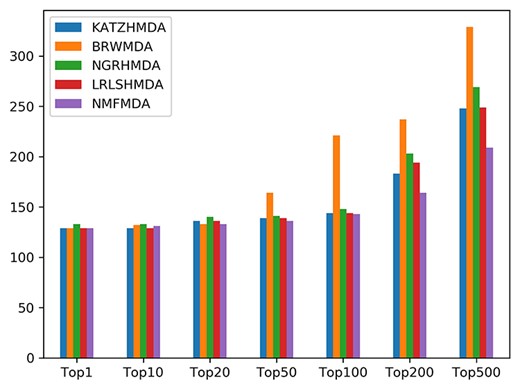
The numbers of correctly predicted MDAs from five representative methods with the global LOOCV.

Open in new tab Download slide

Figure 6

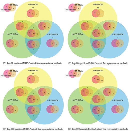
Four overlapping relationships among top 50 (a), top 100 (b), top 200 (c) and top 500 (d) ranked MDAs of five representative methods. The top left Venn diagram of each sub-figure shows the overlapping relationships of high-score MDAs which are just predicted by NGRHMDA and NMFMDA but not by the other three methods. The main Venn diagram of each sub-figure shows the overlapping relationships of high-score MDAs predicted by five methods together.

Open in new tab Download slide

Experimental analysis

From the results of the prediction performances, the random walk methods represented by BRWMDA achieved the best performance among the selected methods in terms of all three validations. The good results are caused by the logistic function and the SNF method, which bring reliable transition matrices for bi-walk [68]. The performances of random walk methods highly depend on the property of the walking network. A well-integrated and informative network leads the walker to a proper destination. The SNF processing captures the vital information and integrates the complementary information from diverse networks by an iterative update based on message-passing [96]. According to Table 3, fusing the Spearman correlation coefficient similarity and the symptom-based disease similarity by the SNF method outperformed all other combinations (AUC = 0.9527), even is better than the original results. It indicates that both the SNF method and the Spearman correlation coefficient similarity generally fit this method, since the iterative fusion approach and the monotonic relationship assessment of two profiles may play an important role in constructing a more reasonable similarity network for walkers [97].

According to the ROC curves in Figure 4, NMFMDA failed to achieve a superior result. However, the matrix factorization methods are common alternatives in other field such as drug–target interaction prediction [32]. Although the MDA matrix factorization is less intuitive as the image decomposition where NMF learns the combination of components, it indeed captures latent properties from both sides. The dissatisfactory prediction result could be partly explained by the unbalanced distribution of associations. A significant fraction of associations are clustered with several common diseases. Hoyer et al. who improve the NMF algorithm by incorporating sparseness constraints provide us with a solution [98]. In our case, the unbalanced distribution (disease-specific centralized distribution of MDAs) simulates a ‘rare’ phenomenon [98]. To overcome this defect, the basis vectors W containing latent properties of diseases should be sparse [98]. Due to this phenomenon, NMFMDA performed better under 5-fold CV when the centralized distribution was alleviated in contrast to LOOCV. Table 3 illustrates that the effect of the GIP kernel similarity far exceeded other similarities. By observing different similarity distributions, the values computed by the GIP kernel similarity were found densely located in the neighborhoods of 0 and 1, having a higher distinguishability, while those computed by the Spearman correlation coefficient similarity mainly ranged from 0 to 0.5. This binary centralized distribution resulting from the GIP kernel similarity may generate sparser basis vectors W in terms of the deduction of the graph regularization term [56, 74, 98]. As a result, matrix factorization methods are not the optimal approach.

Among path-based methods, the representative method, KATZHMDA, did not perform as well as others. It could be explained that the sparse data cause rare paths linking with isolated nodes and therefore these nodes are unable to be identified precisely. It also indicates that path-based methods are more intuitive methods based on the association network. While random walk methods focus on the possible locations that a walker may arrive at, path-based methods pay more attention to the details of all paths. Hence, a convincing roadmap deserves to be assured. However, path across homogeneous networks measured with computational association-based similarities are still not reliable enough due to the computational dimension-reduction deviation during the similarity calculation. The results derived from a series of experiments on different similarity data in Table 3 are supportive evidence for our arguments. When adopting path-based methods, we should concern about new similarity sources and measurements to construct more efficient homogeneous paths like what we tested on extra similarity data.

Relatively, BLMs cover an extensive range of methods based on diverse ideas. From the prediction results of the two selected BLMs, they presented a satisfactory solution to the MDA prediction by taking advantage of disease and microbe similarity information separately. In addition, the further two-step diffusion in NGRHMDA and the modified graph Laplacian regularization term in LRLSHMDA also contribute to the reliable prediction performance. Notably, BLMs are not entirely independent for their processes share mutual associations, but neither of the models participates in the operation of each other until the mergence. We recommend that this approach could be considered as the prime candidate owes to its fast speed and weak dependence on conditional hyperparameters and similarity data as shown in Table 3.

Table 3

Open in new tab

Results of different similarity data applied to typical MDA prediction methods. M: microbe; D: disease; GIP kernel: the GIP kernel similarity; Spearman: the Spearman correlation coefficient similarity; Ave(X + sym): the average of the X similarity and the symptom-based disease similarity and SNF(X + sym): the SNF fusion of the X similarity and the symptom-based disease similarity. We underline the original results and highlight the best result of each method in bold and the global best result in italics

AUC of global/local LOOCV	M: GIP kernel D: GIP kernel	M: Spearman D: Spearman	M: GIP kernel D: Ave (GIP kernel + sym)	M: GIP kernel D: Ave (Spearman + sym)	M: GIP kernel D: SNF (GIP kernel + sym)	M: GIP kernel D: SNF (Spearman + sym)	Average AUC
KATZHMDA	0.8382/0.6806	0.8769/0.5632	0.8644/0.7	0.876/0.5576	0.8786/0.7688	0.8632 /0.5262	0.8662/0.6327
BRWMDA	0.9293/0.8595	0.9406/0.8895	0.922/0.8552	0.9431/0.8861	0.9397/0.8614	*0.9527/0.8894*	0.9379/0.8735
NGRHMDA	0.9111/0.7951	0.8930/0.5967	0.9117/0.7964	0.8943/0.5917	0.9025/0.7889	0.8931/0.6020	0.901/0.6951
LRLSHMDA	0.8909/0.7657	0.8610/0.6429	0.8930/0.7612	0.8429/0.5244	0.8854/0.7367	0.832/0.5222	0.8675/0.6589
NMFMDA	0.8470/0.6973	0.6167/0.4817	0.8568/0.6949	0.6433/ 0.4766	0.8510/0.7012	0.6963/0.4836	0.7519/0.5892
Average AUC	0.8833/0.7596	0.8376/0.6348	0.8896/ 0.7615	0.8399/0.6073	0.8914/0.7714	0.8475/0.6047	0.8649/0.6899

AUC of global/local LOOCV	M: GIP kernel D: GIP kernel	M: Spearman D: Spearman	M: GIP kernel D: Ave (GIP kernel + sym)	M: GIP kernel D: Ave (Spearman + sym)	M: GIP kernel D: SNF (GIP kernel + sym)	M: GIP kernel D: SNF (Spearman + sym)	Average AUC
KATZHMDA	0.8382/0.6806	0.8769/0.5632	0.8644/0.7	0.876/0.5576	0.8786/0.7688	0.8632 /0.5262	0.8662/0.6327
BRWMDA	0.9293/0.8595	0.9406/0.8895	0.922/0.8552	0.9431/0.8861	0.9397/0.8614	*0.9527/0.8894*	0.9379/0.8735
NGRHMDA	0.9111/0.7951	0.8930/0.5967	0.9117/0.7964	0.8943/0.5917	0.9025/0.7889	0.8931/0.6020	0.901/0.6951
LRLSHMDA	0.8909/0.7657	0.8610/0.6429	0.8930/0.7612	0.8429/0.5244	0.8854/0.7367	0.832/0.5222	0.8675/0.6589
NMFMDA	0.8470/0.6973	0.6167/0.4817	0.8568/0.6949	0.6433/ 0.4766	0.8510/0.7012	0.6963/0.4836	0.7519/0.5892
Average AUC	0.8833/0.7596	0.8376/0.6348	0.8896/ 0.7615	0.8399/0.6073	0.8914/0.7714	0.8475/0.6047	0.8649/0.6899

Table 3

Open in new tab

Results of different similarity data applied to typical MDA prediction methods. M: microbe; D: disease; GIP kernel: the GIP kernel similarity; Spearman: the Spearman correlation coefficient similarity; Ave(X + sym): the average of the X similarity and the symptom-based disease similarity and SNF(X + sym): the SNF fusion of the X similarity and the symptom-based disease similarity. We underline the original results and highlight the best result of each method in bold and the global best result in italics

AUC of global/local LOOCV	M: GIP kernel D: GIP kernel	M: Spearman D: Spearman	M: GIP kernel D: Ave (GIP kernel + sym)	M: GIP kernel D: Ave (Spearman + sym)	M: GIP kernel D: SNF (GIP kernel + sym)	M: GIP kernel D: SNF (Spearman + sym)	Average AUC
KATZHMDA	0.8382/0.6806	0.8769/0.5632	0.8644/0.7	0.876/0.5576	0.8786/0.7688	0.8632 /0.5262	0.8662/0.6327
BRWMDA	0.9293/0.8595	0.9406/0.8895	0.922/0.8552	0.9431/0.8861	0.9397/0.8614	*0.9527/0.8894*	0.9379/0.8735
NGRHMDA	0.9111/0.7951	0.8930/0.5967	0.9117/0.7964	0.8943/0.5917	0.9025/0.7889	0.8931/0.6020	0.901/0.6951
LRLSHMDA	0.8909/0.7657	0.8610/0.6429	0.8930/0.7612	0.8429/0.5244	0.8854/0.7367	0.832/0.5222	0.8675/0.6589
NMFMDA	0.8470/0.6973	0.6167/0.4817	0.8568/0.6949	0.6433/ 0.4766	0.8510/0.7012	0.6963/0.4836	0.7519/0.5892
Average AUC	0.8833/0.7596	0.8376/0.6348	0.8896/ 0.7615	0.8399/0.6073	0.8914/0.7714	0.8475/0.6047	0.8649/0.6899

AUC of global/local LOOCV	M: GIP kernel D: GIP kernel	M: Spearman D: Spearman	M: GIP kernel D: Ave (GIP kernel + sym)	M: GIP kernel D: Ave (Spearman + sym)	M: GIP kernel D: SNF (GIP kernel + sym)	M: GIP kernel D: SNF (Spearman + sym)	Average AUC
KATZHMDA	0.8382/0.6806	0.8769/0.5632	0.8644/0.7	0.876/0.5576	0.8786/0.7688	0.8632 /0.5262	0.8662/0.6327
BRWMDA	0.9293/0.8595	0.9406/0.8895	0.922/0.8552	0.9431/0.8861	0.9397/0.8614	*0.9527/0.8894*	0.9379/0.8735
NGRHMDA	0.9111/0.7951	0.8930/0.5967	0.9117/0.7964	0.8943/0.5917	0.9025/0.7889	0.8931/0.6020	0.901/0.6951
LRLSHMDA	0.8909/0.7657	0.8610/0.6429	0.8930/0.7612	0.8429/0.5244	0.8854/0.7367	0.832/0.5222	0.8675/0.6589
NMFMDA	0.8470/0.6973	0.6167/0.4817	0.8568/0.6949	0.6433/ 0.4766	0.8510/0.7012	0.6963/0.4836	0.7519/0.5892
Average AUC	0.8833/0.7596	0.8376/0.6348	0.8896/ 0.7615	0.8399/0.6073	0.8914/0.7714	0.8475/0.6047	0.8649/0.6899

In conclusion, each computational method has its own advantages, applicability and disadvantages. An informative similarity network integrated effectively with prior knowledge could generally improve the prediction results for most methods. Compared with the GIP kernel similarity, the Spearman correlation coefficient similarity fits the methods better based on topological networks (the random walk and path-based methods). Considering the specific predictive capability and the characteristic of each method, it is possible to conduct a combination prediction on the basis of results as shown in Figure 6. Although we analyzed the experimental results by category, we would like to give supplementary explanations on prior experiments: (i) hindered by the unbalanced dataset, we were more focused on comparing computational methods mathematically and horizontally and ignored their biomedical authenticity judged by the empirical validation. This will be discussed in Subsection ‘Biomedical interpretation for computational discovery’. (ii) The prediction accuracy of top-ranked associations is a valuable metric to evaluate the applicability and practical significance of a method. (iii) As shown in Figure 6, the overlapping top-ranked associations predicted by several methods are the highest confidence alternatives for the biomedical validation.

Future work

According to previous studies and our observations, we make some suggestions in perspectives of the data, methods and formulations in order to achieve higher precision, better generalization ability and wider applicability of the MDA prediction in the future.

Enriching data sources

Collecting data from different sources is the top priority which could be divided into two parts. On the one hand, original association data are still sparse and unevenly distributed. So firstly, rigorously verified prediction results could be added to the original association data. A webtool, EviMass, has been developed and conduced to solve this issue [99]. Reported literature will return when users query with an MDA or even association networks. It provides a channel for biologists to test their hypotheses by mining biomedical evidence. Secondly, searching recent related literature for a novel association data is necessary. For example, Yan et al. extended the MDA dataset as HMDAD-SUP [89]. Furthermore, the MDA prediction prefers more independent datasets for training and testing models. For example, Janssens et al. constructed the Disbiome database which continuously organizes experimental cases linking the microorganism to disease from PubMed publications [100]. Recently, an insightful review meticulously outlined existing knowledge bases of human MDAs and discussed current challenges in the process of constructing them [101]. Readers can obtain relevant information of natural language processing, text mining, terminology unification and data consolidation to have an overall grasp on a new MDA-related knowledge base.

On the other hand, multi-source data need to be introduced to enhance the generalization performance and support innovative approaches. For example, other data for similarity, including GDA, symptom-based disease similarity and so on [36, 40, 46, 47, 53, 89], have been successfully applied to the MDA prediction. However, these data could also be used as microbe and disease features in feature-based learning models. Likewise, other microbe-related and disease-related information that could identify a microorganism or a disease should be considered in the MDA prediction. For example, PHI-base stores a lot of genetic information about pathogens and their various mutant phenotypes [102]. EuPathDB is a large-scale retrieval platform for eukaryotic microbes, serving to identify genes with an all-round search strategy [103]. The therapeutic drug list of a given disease can be retrieved in KEGG [104].

There is yet no certain microbe-disease non-association dataset to date. The label ‘0’ has two possible interpretations, unknown association or non-association. It affects the effectiveness of supervised learning methods. Although some technical solutions have already been proposed in ABHMDA (balanced sampling from bi-class sets) [87], BMCMDA (unobserved states with the probability of being non-associations) [88] and other studies (in silico screening) [105, 106], it is necessary to curate verified non-association entries manually.

Unifying taxonomy and terminology

Another measure for the enhancement of prediction reliability is to define the taxonomic level of each microorganism and perform the prediction at the same level [71]. Organisms could be classified and mapped with taxonomy (e.g. NCBI [107] and SILVA [21] taxonomy). Moreover, the introduction of taxonomy would facilitate a precise identification of microorganisms among microbiology databases, which aids in incorporating microbiome (e.g. microbial genome sequences [21, 22] and patient-derived microbial metagenome [22, 108], transcriptome and metabolome [24–26]) into the MDA prediction. Microbiomic data could be used to identify microorganisms and measure inter-microorganism similarities, whereas relevant work has been done with the aim at predicting virus-host associations. Ahlgren et al. measured inter-viruses dissimilarities utilizing genomic oligonucleotide frequencies and Liu et al. constructed the virus similarity network based on the prediction of virus-host associations, which provide examples of using microbiome in microbe-related association prediction [109, 110].

Additionally, it is necessary to expand the current size of diseases and requires a basic terminology dictionary to regulate disease synonyms and classifications [101]. Because of complex aliases, extended description (e.g. ‘new-onset untreated’ rheumatoid arthritis) and ambiguity between symptoms and diseases [38], hierarchical classifications, such as Medical Dictionary for Regulatory Activities [111] and MeSH [112] are required. They could contribute in organizing disease terms with a structured standard and hence allow to retrieve standardized disease terms from different disease repositories in a consistent way.

Introducing deep learning methods

Machine learning is a powerful tool, and related algorithms have been widely applied to our issue, such as least squares, matrix factorization and completion. However, feature-based machine learning algorithms are trapped in the dilemma of lacking effective features and hence received little attention. Compared with machine learning, deep learning, which is regarded as a meaningful attempt, has not yet been introduced into MDA prediction. In response to the dilemma above, deep learning-based algorithms that target a complicated topological network and capture its node embeddings have been proposed in many studies [113–118].

Inspired by representation learning such as DeepWalk [115], refining characteristics of the topological structure of the MDA network by deep learning methods is an available way to obtain distinctive representations. For example, Masashi et al. extracted topological information from the drug molecular structure by encoding all atoms and chemical bonds in a variable dimensional space. They then converted these stochastic pre-encodings to final molecular embeddings in the form of vector representations by the graph neural network [119]. In our case, a microbe or disease node can be represented as the co-contribution of its neighbors and itself in the homogeneous network through graph neural networks, and then the end-to-end model is a preferred choice for handling the subsequent prediction.

Furthermore, Zitnik et al. proposed an approach for modeling a node encoder in the heterogeneous network constituted of multigraph convolutional networks [120]. When we introduce new interactive networks into the MDA prediction, the encoder integrating multi-graph information for a node would take effect. Although topography-based deep learning methods mentioned above, especially the graph neural network, are effective tools, these types of methods are unable to predict novel associations because the encoding dictionary (or one-hot codes) is pre-fixed. Hence, it is urgent to curate valid features capable of identifying a microorganism or a disease.

Fusing multi-source similarities in an effective manner is also an essential task that we can apply deep learning methods to. For example, Zeng et al. assembled 10 types of drug-drug networks and converted them to a common feature space that generates reconstructed drug features via multi-modal deep autoencoder [121]. The step of aggregating similarity features could be addressed by multi-input concatenation or summation layer.

Evaluating diversely

Comprehensively, evaluating prediction methods is also a critical part of the MDA prediction. In this article, we mainly focus on discussing non-feature-based prediction methods. These methods require a reconstruction of the association matrix via removing label ‘1’ when testing novel associations. Therefore, the association matrix changes by different test sampling modes. In order to evaluate the prediction ability comprehensively, more test sampling modes should be designed besides CVs. For example, to evaluate the capability of predicting associations of a new disease with known microbes (or vice versa), the corresponding profile should be excluded from the association matrix and recovered by a set of predicted scores. Note that supplementary similarities (i.e. based on data mentioned in Section ‘DATA’) are still available for predicting new diseases and microbes. Besides probabilistic outcome for a pair of microbe-disease, we could further determine a threshold to estimate whether they associate by maximizing the Matthews correlation coefficient [122] theoretically, which could serve as an evaluation metric other than the rank.

Reforming predictive tasks

The MDA prediction is a typical binary classification task but able to develop a much finer-grained prediction. Predicting drug–target binding affinities, for example, is a further work based on drug–target interaction prediction [123]. HMDAD records additional entries whether the quantity of microbial population is increased or decreased in the reported cases [29]. Furthermore, the Disbiome database provides the microbial population variation between control-derived and patient-derived groups [100]. Most of population indexes are given in the absolute quantitative value responded in a given unit (the unit is dependent on the used detection method) [100]. Such quantitative relationships could be used for predicting disease-induced microbial population variations, physiological disorders in response to microbial population dynamics, inter-microbe interactions and even synergisms in combinations of human microbiota in the future.

The network analysis is a worthwhile strategy that further extends more refined prediction tasks methodologically for a better mechanistic inference. On the one hand, applying network analysis to the combined heterogeneous network is a popular trend along with the enrichment of microbe-centric and disease-centric networks. Microbe-centric networks (e.g. microbe co-occurrence [124, 125], microbe-gene [22], microbe-protein [44] and microbe-host [126]) and disease-centric networks (e.g. disease-gene [34, 127], disease-symptom [38] and disease-drug [128, 129]) could cooperate to construct a comprehensive relational database based on MDAs. This is a challenging task requiring the screening and consolidation of these massive data based on specialized knowledge. On the other hand, the network analysis has been more common in studying community-level microbiome-host relationships to explain pathogenesis [130]. For example, a literature-curated network, composed of the gut microbiome and host cells that metabolically interact annotated with small-molecule transport and macromolecule degradation events, has been constructed and serves to reveal microbial metabolism functionally for a specific disease [131]. Additionally, identifying enzyme-coding genes and their annotated enzymes from microbial metagenomics data derived from healthy individuals and diseased individuals has been used to compare topological differences based on metabolic networks [132]. These networks take enzymes as nodes, and there is an edge between two enzymes if they catalyze successive reactions. These studies indicate that networks constructed of a given population-derived microbiomic data truly help to analyze and infer disease mechanisms, which is worthy of consideration for predictive tasks ahead.

Developing related tools

There are only a few web-based platforms where researchers can perform a customized MDA prediction. For instance, MicroPattern is a web-based tool that divides microorganisms into different disease-related sets for reference and provides the function of similarity calculation [133]. Such platforms have integrated various state-of-the-art prediction methods, which are specialized for other fields (e.g. meta-PPISP [134], DINIES [135] and DIANA-microT [136]). However, we could not ignore other related works which explore microbe-disease and microbe-host relationships. For example, an open-source pipeline, MicroPro, can estimate abundance profiles of unknown microbial organisms based on unmapped reads from the metagenomic data and predict phenotypes using complete abundance profiles of the cases and the controls [137]. Furthermore, an online tool, NetCooperate, can quantify the ability of the nutritive support of a host for a parasitic or commensal organism and the complementarity of a pair of microorganisms based on their metabolic networks [138]. Such open web-based platforms and available software packages truly facilitate further studies of microorganism–human relationships from both methodological and biomedical perspectives.

Biomedical interpretation for computational discovery

A pair of high-confidence MDA could be interpreted from two biomedical perspectives as follows: (i) species-specific changes in microbial community composition are found within patients, but there is no evidence to suggest that it is a pathogen or even a diagnostic signature [139]. (ii) It is a pathogen [140]. The pathogenicity is not the intrinsic nature of microorganisms, and the host response to potential virulence factors varies [141]. More importantly, identifying the causality of microbe-outcome relationships is sometimes unrealistic [142]. Therefore, interpreting any computational discovery is a complex and tough work. When obtaining potential candidates, computational scientists usually seek for empirical literature to conduct case studies [72]. However, biologists can purposefully identify species-specific microbial biomarkers from the host response and link microorganism to disease with the novel computational discovery [143]. Based on this, biologists and bioinformaticians can work together and carry out a thorough research on the detailed mechanism, combining the subjects such as genetics, metabolism, toxicology and so on. For example, considering genetic and metabolic strategies of microbiota, biologists curated organ-specific and patient-specific microbial community-level metabolic networks and developed computational frameworks to study the biomedical interpretation of specific microbial impact on human health [131, 132]. Additionally, some biologists have modelled dynamic simulators based on immune responses and environment-driven microbial behaviors for the pathological interpretation. For example, Wendelsdorf et al. developed a gastrointestinal immune system simulator and applied it to find a treatment strategy for Brachyispira hyodysenteriae infection-induced dysentery [144]. The agent-based models have been established to study gastrointestinal cell-pathogen interaction mechanisms of Pseudomonas aeruginosa and Helicobacter pylori from the aspects of pathway regulation of immunity and virulence [145, 146]. The shift of computational discovery to biomedical discovery heavily relies on expert experiences. Therefore, computational scientists are encouraged to increase the accessibility of the MDA discovery to biomedical research community.

Conclusion

The MDA prediction is critical in revealing relationships between human diseases and microorganisms. In this study, a comprehensive overview of the MDA prediction has been given. Firstly, we introduced multi-source data applied for the MDA prediction and their purposes, respectively. Secondly, we described several similarity calculation methods that are widely used in the MDA prediction. We then classified computational prediction methods and give detailed descriptions of them. Meanwhile, we conducted a comparative assessment of similarity calculation methods and computational prediction methods and then analyzed their prediction performances. Finally, we offered a series of recommendations on enhancing the prediction performance and discussed top tasks in the future.

The development of sequencing technologies lays the basis for conducting a detection in microorganism population abundance [147]. High-throughput sequencing technologies and advanced omics technologies allow diversified means to detect the changes in patient-derived microbial composition [148]. However, these data are still deficient with the problems of information loss, sparsity, small-scale data, unbalanced distribution, lack of a unified taxonomic standard and ambiguity in disease terms at this stage. The problems of small-scale data and unregulated use of terms need the most attention. Enriching data, introducing the taxonomy and the terminology dictionary and performing fine-grained predictions are effective approaches to alleviate these problems. Each method proposed its unique strategy by adopting, integrating, improving and inventing algorithms adapted to our issue. Besides the methodology, we should also guide future efforts to a practical and broad direction like the instances that we talked over in future work. Microbe-related association prediction is a rising research field and has broad prospects of development and application because its interdisciplinary perspective relates to fields including medication [149], genome [150], pathogenesis [151] and phenotype [152]. It is to be expected that more and more advanced computational methods as well as comprehensive datasets will be developed in the future.

Key Points

The microbe-disease association (MDA) prediction is an in silico pre-screening instrument for the clinical trials of pathogenic mechanisms related to microorganisms. Various raw data used for predicting MDAs and computational similarity pre-processes methods are summarized.
Computational MDA prediction methods based on diverse strategies and algorithms, to our knowledge, are classified and elaborated. A series of experiments with different combinations of prediction methods and similarity data are performed. An analysis of the results and possible improvement based on their nature are discussed.
Considering the small-scale dataset and the lack of feature data, data enrichment and regularization are the prime tasks that could be ameliorated in many ways. Deep learning technologies can help address it by learning latent topological information based on the MDA network structure, and more machine learning models are encouraged to be proposed and adopted as the data are expanded and regularized.
Concerning further work after the MDA prediction, quantitative records of the microbial population variation in experimental cases enable the models to perform fine-grained prediction tasks, and the network analysis could be applied to the inference of microbiological pathogenesis with annotated networks of biological events in the future.

Funding

NSFC-Zhejiang Joint Fund for the Integration of Industrialization and Informatization under grant No. U1909208, National Natural Science Foundation of China (grant nos. 61772552, 61962050); 111 Project (grant no. B18059); Hunan Provincial Science and Technology Program (grant no. 2018WK4001).

Conflict of Interest

None declared.

Zhongqi Wen is a graduate student in the Hunan Provincial Key Lab of Bioinformatics, School of Computer Science and Engineering at Central South University, Hunan, China. His research interests include microbe-related and drug toxicity prediction.

Cheng Yan is currently a postdoctoral in the School of Computer Science and Engineering, Central South University, Changsha, Hunan, China. His current research interests include bioinformatics and machine learning.

Guihua Duan is an Associate Professor in the School of Computer Science and Engineering, Central South University. Her research interests include bioinformatics, network security and computer network.

Suning Li is a Research Assistant in the Hunan Provincial Key Lab of Bioinformatics, School of Computer Science and Engineering, Central South University, Changsha, Hunan, China.

Fang-Xiang Wu is a Professor in the College of Engineering and the Department of Computer Sciences, University of Saskatchewan, Saskatoon, Canada. His research interests include artificial intelligence and computational biology.

Jianxin Wang is a Professor in the Hunan Provincial Key Lab of Bioinformatics, School of Computer Science and Engineering at Central South University, Hunan, China. His research interests include computational genomics and proteomics.

References

1.

Huttenhower

C

,

Gevers

D

,

Knight

R

, et al.

Structure, function and diversity of the healthy human microbiome

.

Nature

2012

;

486

(

7402

):

207

–

14

.

Google Scholar

PubMed

OpenURL Placeholder Text

WorldCat

2.

Gill

SR

,

Pop

M

,

DeBoy

RT

, et al.

Metagenomic analysis of the human distal gut microbiome

.

Science

2006

;

312

(

5778

):

1355

–

9

.

3.

Marco

ML

,

Heeney

D

,

Binda

S

, et al.

Health benefits of fermented foods: microbiota and beyond

.

Curr Opin Biotechnol

2017

;

44

:

94

–

102

.

4.

Hooper

LV

,

Littman

DR

,

Macpherson

AJ

.

Interactions between the microbiota and the immune system

.

Science

2012

;

336

(

6086

):

1268

–

73

.

5.

Mazmanian

SK

,

Liu

CH

,

Tzianabos

AO

, et al.

An immunomodulatory molecule of symbiotic bacteria directs maturation of the host immune system

.

Cell

2005

;

122

(

1

):

107

–

18

.

6.

Bouskra

D

,

Brézillon

C

,

Bérard

M

, et al.

Lymphoid tissue genesis induced by commensals through NOD1 regulates intestinal homeostasis

.

Nature

2008

;

456

(

7221

):

507

.

7.

Petrova

MI

,

Lievens

E

,

Malik

S

, et al.

Lactobacillus species as biomarkers and agents that can promote various aspects of vaginal health

.

Front Physiol

2015

;

6

:

81

.

8.

Wang

ZK

,

Yang

YS

,

Stefka

AT

, et al.

Fungal microbiota and digestive diseases

.

Aliment Pharmacol Ther

2014

;

39

(

8

):

751

–

66

.

9.

Brandl

K

,

Plitas

G

,

Schnabl

B

, et al.

MyD88-mediated signals induce the bactericidal lectin RegIIIγ and protect mice against intestinal listeria monocytogenes infection

.

J Exp Med

2007

;

204

(

8

):

1891

–

900

.

10.

Jesmok

EM

,

Hopkins

JM

,

Foran

DR

.

Next-generation sequencing of the bacterial 16S rRNA gene for forensic soil comparison: a feasibility study

.

J Forensic Sci

2016

;

61

(

3

):

607

–

17

.

11.

Ranjan

R

,

Rani

A

,

Metwally

A

, et al.

Analysis of the microbiome: advantages of whole genome shotgun versus 16S amplicon sequencing

.

Biochem Biophys Res Commun

2016

;

469

(

4

):

967

–

77

.

12.

Laureano

AC

,

Schwartz

RA

,

Cohen

PJ

.

Facial bacterial infections: folliculitis

.

Clin Dermatol

2014

;

32

(

6

):

711

–

4

.

13.

Colombo

APV

,

Boches

SK

,

Cotton

SL

, et al.

Comparisons of subgingival microbial profiles of refractory periodontitis, severe periodontitis, and periodontal health using the human oral microbe identification microarray

.

J Periodontol

2009

;

80

(

9

):

1421

–

32

.

14.

Jorth

P

,

Turner

KH

,

Gumus

P

, et al.

Metatranscriptomics of the human oral microbiome during health and disease

.

MBio

2014

;

5

(

2

):

e01012

–

4

.

15.

Hold

GL

,

Smith

M

,

Grange

C

, et al.

Role of the gut microbiota in inflammatory bowel disease pathogenesis: what have we learnt in the past 10 years?

World J Gastroenterol: WJG

2014

;

20

(

5

):

1192

.

Google Scholar

Crossref

WorldCat

16.

Li

J

,

Zhao

F

,

Wang

Y

, et al.

Gut microbiota dysbiosis contributes to the development of hypertension

.

Microbiome

2017

;

5

(

1

):

14

.

17.

Louis

P

,

Hold

GL

,

Flint

HJ

.

The gut microbiota, bacterial metabolites and colorectal cancer

.

Nat Rev Microbiol

2014

;

12

(

10

):

661

–

72

.

18.

Zhao

L

.

The gut microbiota and obesity: from correlation to causality

.

Nat Rev Microbiol

2013

;

11

(

9

):

639

–

47

.

19.

Chen

T

,

Yu

W-H

,

Izard

J

, et al.

The human oral microbiome database: a web accessible resource for investigating oral microbe taxonomic and genomic information

.

Database

2010

;

2010

:baq013.

Google Scholar

OpenURL Placeholder Text

WorldCat

20.

Matsumoto

M

,

Sakamoto

M

,

Hayashi

H

, et al.

Novel phylogenetic assignment database for terminal-restriction fragment length polymorphism analysis of human colonic microbiota

.

J Microbiol Methods

2005

;

61

(

3

):

305

–

19

.

21.

Quast

C

,

Pruesse

E

,

Yilmaz

P

, et al.

The SILVA ribosomal RNA gene database project: improved data processing and web-based tools

.

Nucleic Acids Res

2012

;

41

(

D1

):

D590

–

6

.

22.

Chen

I-MA

,

Chu

K

,

Palaniappan

K

, et al.

IMG/M v. 5.0: an integrated data management and comparative analysis system for microbial genomes and microbiomes

.

Nucleic Acids Res

2019

;

47

(

D1

):

D666

–

77

.

23.

Finn

RD

,

Coggill

P

,

Eberhardt

RY

, et al.

The Pfam protein families database: towards a more sustainable future

.

Nucleic Acids Res

2016

;

44

(

D1

):

D279

–

85

.

24.

Faith

JJ

,

Driscoll

ME

,

Fusaro

VA

, et al.

Many microbe microarrays database: uniformly normalized Affymetrix compendia with structured experimental metadata

.

Nucleic Acids Res

2007

;

36

(

1

):

866

–

70

.

Google Scholar

OpenURL Placeholder Text

WorldCat

25.

Ulrich

LE

,

Zhulin

IB

.

MiST: a microbial signal transduction database

.

Nucleic Acids Res

2007

;

35

(

suppl_1

):

D386

–

90

.

Google Scholar

PubMed

OpenURL Placeholder Text

WorldCat

26.

Saier

MH

, Jr,

Reddy

VS

,

Tamang

DG

, et al.

The transporter classification database

.

Nucleic Acids Res

2014

;

42

(

D1

):

D251

–

8

.

27.

Coelho

ED

,

Santiago Ae

M

,

Arrais

JP

, et al.

Computational methodology for predicting the landscape of the human--microbial interactome region level influence

.

J Bioinform Comput Biol

2015

;

13

(

05

):

1550023

.

28.

Turnbaugh

PJ

,

Ley

RE

,

Hamady

M

, et al.

The human microbiome project

.

Nature

2007

;

449

(

7164

):

804

.

29.

Ma

W

,

Zhang

L

,

Zeng

P

, et al.

An analysis of human microbe--disease associations

.

Brief Bioinform

2016

;

18

(

1

):

85

–

97

.

30.

Richard

CL

,

Blay

J

.

Thiazolidinedione drugs down-regulate CXCR4 expression on human colorectal cancer cells in a peroxisome proliferator activated receptor γ-dependent manner

.

Int J Oncol

2007

;

30

(

5

):

1215

–

22

.

Google Scholar

PubMed

OpenURL Placeholder Text

WorldCat

31.

Svacina

S

.

Colorectal cancer and diabetes

.

Vnitrni lekarstvi

2011

;

57

(

4

):

378

–

80

.

Google Scholar

PubMed

OpenURL Placeholder Text

WorldCat

32.

Ezzat

A

,

Wu

M

,

Li

X-L

, et al.

Computational prediction of drug-target interactions using chemogenomic approaches: an empirical survey

.

Brief Bioinform

2019

;

20

(

4

):

1337

–

57

.

33.

Zou

Q

,

Li

J

,

Song

L

, et al.

Similarity computation strategies in the microRNA-disease network: a survey

.

Brief Funct Genomics

2015

;

15

(

1

):

55

–

64

.

Google Scholar

PubMed

OpenURL Placeholder Text

WorldCat

34.

Piñero

J

,

Bravo

Á

,

Queralt-Rosinach

N

, et al.

DisGeNET: a comprehensive platform integrating information on human disease-associated genes and variants

.

Nucleic Acids Res

2016

;

gkw943

.

Google Scholar

OpenURL Placeholder Text

WorldCat

35.

Bravo

Á

,

Piñero

J

,

Queralt-Rosinach

N

, et al.

Extraction of relations between genes and diseases from text and large-scale data analysis: implications for translational research

.

BMC Bioinformatics

2015

;

16

(

1

):

55

.

36.

Wang

L

,

Ping

P

,

Kuang

L

, et al.

A novel approach based on bipartite network to predict human microbe-disease associations

.

Current Bioinformatics

2018

;

13

(

2

):

141

–

8

.

Google Scholar

Crossref

WorldCat

37.

Wheeler

DL

,

Church

DM

,

Federhen

S

, et al.

Database resources of the National Center for biotechnology

.

Nucleic Acids Res

2003

;

31

(

1

):

28

–

33

.

38.

Zhou

X

,

Menche

J

,

Barabási

A-L

, et al.

Human symptoms--disease network

.

Nat Commun

2014

;

5

:

4212

.

39.

Salton

G

,

Wong

A

,

Yang

C-S

.

A vector space model for automatic indexing

.

Commun ACM

1975

;

18

(

11

):

613

–

20

.

Google Scholar

Crossref

WorldCat

40.

Chen

X

,

Huang

Y-A

,

You

Z-H

, et al.

A novel approach based on KATZ measure to predict associations of human microbiota with non-infectious diseases

.

Bioinformatics

2016

;

33

(

5

):

733

–

9

.

Google Scholar

OpenURL Placeholder Text

WorldCat

41.

Lowe

HJ

,

Barnett

GO

.

Understanding and using the medical subject headings (MeSH) vocabulary to perform literature searches

.

JAMA

1994

;

271

(

14

):

1103

–

8

.

42.

Schriml

LM

,

Mitraka

E

,

Munro

J

, et al.

Human disease ontology 2018 update: classification, content and workflow expansion

.

Nucleic Acids Res

2019

;

47

(

D1

):

D955

–

62

.

43.

Wang

D

,

Wang

J

,

Lu

M

, et al.

Inferring the human microRNA functional similarity and functional network based on microRNA-associated diseases

.

Bioinformatics

2010

;

26

(

13

):

1644

–

50

.

44.

Szklarczyk

D

,

Gable

AL

,

Lyon

D

, et al.

STRING v11: protein–protein association networks with increased coverage, supporting functional discovery in genome-wide experimental datasets

.

Nucleic Acids Res

2019

;

47

(

D1

):

D607

–

13

.

45.

Kamneva

OK

.

Genome composition and phylogeny of microbes predict their co-occurrence in the environment

.

PLoS Comput Biol

2017

;

13

(

2

):

e1005366

.

46.

Fan

C

,

Lei

X

,

Guo

L

, et al.

Predicting the associations between microbes and diseases by integrating multiple data sources and path-based HeteSim scores

.

Neurocomputing

2019

;

323

:

76

–

85

.

Google Scholar

Crossref

WorldCat

47.

Long

Y

,

Luo

J

.

WMGHMDA: a novel weighted meta-graph-based model for predicting human microbe-disease association on heterogeneous information network

.

BMC Bioinformatics

2019

;

20

(

1

):

541

.

48.

van Laarhoven

T

,

Nabuurs

SB

,

Marchiori

E

.

Gaussian interaction profile kernels for predicting drug--target interaction

.

Bioinformatics

2011

;

27

(

21

):

3036

–

43

.

49.

Wu

C

,

Gao

R

,

Zhang

D

, et al.

PRWHMDA: human microbe-disease association prediction by random walk on the heterogeneous network with PSO

.

Int J Biol Sci

2018

;

14

(

8

):

849

–

57

.

50.

Faust

K

,

Raes

J

.

Microbial interactions: from networks to models

.

Nat Rev Microbiol

2012

;

10

(

8

):

538

–

50

.

51.

Shen

X

,

Chen

Y

,

Jiang

X

, et al. Predicting disease-microbe association by random walking on the heterogeneous network. In:

Bioinformatics and Biomedicine (BIBM), 2016 IEEE International Conference on

2016

, pp.

771

–

4

.

52.

Shen

X

,

Chen

Y

,

Jiang

X

, et al.

Prioritizing disease-causing microbes based on random walking on the heterogeneous network

.

Methods

2017

;

124

:

120

–

5

.

53.

Zhang

W

,

Yang

W

,

Lu

X

, et al.

The bi-direction similarity integration method for predicting microbe-disease associations

.

IEEE Access

2018

;

6

:

38052

–

61

.

Google Scholar

Crossref

WorldCat

54.

Van Driel

MA

,

Bruggeman

J

,

Vriend

G

, et al.

A text-mining analysis of the human phenome

.

Eur J Hum Genet

2006

;

14

(

5

):

535

.

55.

Vanunu

O

,

Magger

O

,

Ruppin

E

, et al.

Associating genes and protein complexes with disease via network propagation

.

PLoS Comput Biol

2010

;

6

(

1

):

e1000641

.

56.

Liu

Y

,

Wang

S-L

,

Zhang

J-F

.

Prediction of microbe--disease associations by graph regularized non-negative matrix factorization

.

J Comput Biol

2018

;

25

(

12

):

1385

–

94

.

Google Scholar

Crossref

WorldCat

57.

Xie

M

,

Liu

X

,

Li

S

.

A novel approach based on bipartite network recommendation and KATZ model to predict potential micro-disease associations

.

Front Genet

2019

;

10

:

1147

.

Google Scholar

PubMed

OpenURL Placeholder Text

WorldCat

58.

Zou

S

,

Zhang

J

,

Zhang

Z

.

A novel approach for predicting microbe-disease associations by bi-random walk on the heterogeneous network

.

PLoS One

2017

;

12

(

9

):

e0184394

.

59.

He

B-S

,

Peng

L-H

,

Li

Z

.

Human microbe-disease association prediction with graph regularized non-negative matrix factorization

.

Front Microbiol

2018

;

9

:

2056

.

Google Scholar

PubMed

OpenURL Placeholder Text

WorldCat

60.

Lee

H

,

Wang

Y

,

Wang

L

, et al.

A novel human microbe-disease association prediction method based on the bidirectional weighted network

.

Front Microbiol

2019

;

10

:

676

.

Google Scholar

PubMed

OpenURL Placeholder Text

WorldCat

61.

Katz

L

.

A new status index derived from sociometric analysis

.

Psychometrika

1953

;

18

(

1

):

39

–

43

.

Google Scholar

Crossref

WorldCat

62.

Junker

BH

,

Schreiber

F

.

Analysis of Biological Networks

.

Weinheim, Germany: John Wiley & Sons

,

2011

.

Google Scholar

Google Preview

OpenURL Placeholder Text

WorldCat

63.

Huang

Z-A

,

Chen

X

,

Zhu

Z

, et al.

PBHMDA: path-based human microbe-disease association prediction

.

Front Microbiol

2017

;

8

:

233

.

Google Scholar

PubMed

OpenURL Placeholder Text

WorldCat

64.

Shi

C

,

Kong

X

,

Huang

Y

, et al.

Hetesim: a general framework for relevance measure in heterogeneous networks

.

IEEE Trans Knowl Data Eng

2014

;

26

(

10

):

2479

–

92

.

Google Scholar

Crossref

WorldCat

65.

Luo

J

,

Long

Y

.

NTSHMDA: prediction of human microbe-disease association based on random walk by integrating network topological similarity

.

IEEE/ACM Trans Comput Biol Bioinform

2018

, doi:

10.1109/TCBB.2018.2883041

.

Google Scholar

OpenURL Placeholder Text

WorldCat

Crossref

66.

Niu

Y

,

Wang

G

,

Qu

C

, et al.

RWHMDA: random walk on Hypergraph for microbe-disease association prediction

.

Front Microbiol

2019

;

10

:

1578

.

67.

Wang

L

,

Wang

Y

,

Li

H

, et al.

A bidirectional label propagation based computational model for potential microbe-disease association prediction

.

Front Microbiol

2019

;

10

:

684

.

68.

Yan

C

,

Duan

G

,

Wu

F

, et al.

BRWMDA: predicting microbe-disease associations based on similarities and bi-random walk on disease and microbe networks

.

IEEE/ACM Trans Comput Biol Bioinform

2019

, doi:

10.1109/TCBB.2019.2907626

.

Google Scholar

OpenURL Placeholder Text

WorldCat

Crossref

69.

Shen

X

,

Zhu

H

,

Jiang

X

, et al. A Novel Approach Based on Bi-Random Walk to Predict Microbe-Disease Associations. In:

International Conference on Intelligent Computing

,

2018

, pp.

746

–

52

.

70.

Huang

Y-A

,

You

Z-H

,

Chen

X

, et al.

Prediction of microbe--disease association from the integration of neighbor and graph with collaborative recommendation model

.

J Transl Med

2017

;

15

(

1

):

209

.

71.

Zou

S

,

Zhang

J

,

Zhang

Z

.

Novel human microbe-disease associations inference based on network consistency projection

.

Sci Rep

2018

;

8

(

1

):

8034

.

72.

Wang

F

,

Huang

Z-A

,

Chen

X

, et al.

LRLSHMDA: laplacian regularized least squares for human microbe--disease association prediction

.

Sci Rep

2017

;

7

(

1

):

7601

.

73.

Chung

FR

,

Graham

FC

.

Spectral graph theory

. Providence, RI: American Mathematical Soc.,

1997

.

OpenURL Placeholder Text

WorldCat

74.

Cai

D

,

He

X

,

Han

J

, et al.

Graph regularized nonnegative matrix factorization for data representation

.

IEEE Trans Pattern Anal Mach Intell

2011

;

33

(

8

):

1548

–

60

.

Google Scholar

PubMed

OpenURL Placeholder Text

WorldCat

75.

Li

L-X

,

Wu

L

,

Zhang

H-S

, et al.

A fast algorithm for nonnegative matrix factorization and its convergence

.

IEEE T Neur Net Lear

2014

;

25

(

10

):

1855

–

63

.

Google Scholar

Crossref

WorldCat

76.

Tian

L-P

,

Luo

P

,

Wang

H

, et al.

CASNMF: a converged algorithm for symmetrical nonnegative matrix factorization

.

Neurocomputing

2018

;

275

:

2031

–

40

.

Google Scholar

Crossref

WorldCat

77.

Lee

DD

,

Seung

HS

.

Learning the parts of objects by non-negative matrix factorization

.

Nature

1999

;

401

(

6755

):

788

.

78.

Guan

N

,

Tao

D

,

Luo

Z

, et al.

Manifold regularized discriminative nonnegative matrix factorization with fast gradient descent

.

IEEE Trans Image Process

2011

;

20

(

7

):

2030

–

48

.

79.

Ezzat

A

,

Zhao

P

,

Wu

M

, et al.

Drug-target interaction prediction with graph regularized matrix factorization

.

IEEE ACM T Comput Bi

2017

;

14

(

3

):

646

–

56

.

Google Scholar

OpenURL Placeholder Text

WorldCat

80.

Shen

Z

,

Jiang

Z

,

Bao

W.

CMFHMDA: Collaborative matrix factorization for human microbe-disease association prediction. In:

International Conference on Intelligent Computing

,

2017

, pp.

261

–

9

.

81.

Pech

R

,

Hao

D

,

Po

M

, et al.

Predicting drug-target interactions via sparse learning

.

Drugs

2017

;

801

(

445

):

210

.

Google Scholar

OpenURL Placeholder Text

WorldCat

82.

Qu

J

,

Zhao

Y

,

Yin

J

.

Identification and analysis of human microbe-disease associations by matrix decomposition and label propagation

.

Front Microbiol

2019

;

10

:291.

Google Scholar

OpenURL Placeholder Text

WorldCat

83.

Meng

F

,

Yang

X

,

Zhou

C

.

The augmented Lagrange multipliers method for matrix completion from corrupted samplings with application to mixed Gaussian-impulse noise removal

.

PLoS One

2014

;

9

(

9

):

e108125

.

84.

Chen

S

,

Liu

D

,

Zheng

J

et al. Predicting microbe-disease association by kernelized Bayesian matrix factorization. In:

International Conference on Intelligent Computing

,

2018

, pp.

389

–

94

.

85.

Gönen

M

.

Predicting drug–target interactions from chemical and genomic kernels using Bayesian matrix factorization

.

Bioinformatics

2012

;

28

(

18

):

2304

–

10

.

86.

Wu

C

,

Gao

R

,

Zhang

Y

.

mHMDA: human microbe-disease association prediction by matrix completion and multi-source information

.

IEEE Access

2019

;

7

:

106687

–

93

.

Google Scholar

Crossref

WorldCat

87.

Peng

L-H

,

Yin

J

,

Zhou

L

, et al.

Human microbe-disease association prediction based on adaptive boosting

.

Front Microbiol

2018

;

9

:

2440

.

88.

Shi

J-Y

,

Huang

H

,

Zhang

Y-N

, et al.

BMCMDA: a novel model for predicting human microbe-disease associations via binary matrix completion

.

BMC Bioinformatics

2018

;

19

(

9

):

169

.

Google Scholar

PubMed

OpenURL Placeholder Text

WorldCat

89.

Yan

C

,

Duan

G

,

Wu

F

, et al.

MCHMDA: predicting microbe-disease associations based on similarities and low-rank matrix completion

.

IEEE/ACM Trans Comput Biol Bioinform

2019

, doi:

10.1109/TCBB.2019.2926716

.

Google Scholar

OpenURL Placeholder Text

WorldCat

Crossref

90.

Cai

J-F

,

Candès

EJ

,

Shen

Z

.

A singular value thresholding algorithm for matrix completion

.

SIAM J Optimiz

2010

;

20

(

4

):

1956

–

82

.

Google Scholar

Crossref

WorldCat

91.

Uzawa

AH

.

Studies in Linear and Nonlinear Programming

. Stanford, CA: Stanford University Press,

1958

.

92.

Yin

W

,

Osher

S

,

Darbon

J

, et al.

Bregman iterative algorithms for compressed sensing and related problems

.

SIAM J Imaging Sciences

2008

;

1

(

1

):

143

–

68

.

Google Scholar

Crossref

WorldCat

93.

Kohavi

R.

A study of cross-validation and bootstrap for accuracy estimation and model selection. In:

International Joint Conference on Articial Intelligenc

,

1995

, pp.

1137

–

1145

.

Montreal, Canada

.

94.

Hanley

J

,

McNeil

B

.

The meaning and use of the area under a receiver operating characteristic (ROC) curve

.

Radiology

1982

;

143

(

1

):

29

–

36

.

95.

Mason

SJ

,

Graham

NE

.

Areas beneath the relative operating characteristics (ROC) and relative operating levels (ROL) curves: statistical significance and interpretation

.

Q J Roy Meteorol Soc

2002

;

128

(

584

):

2145

–

66

.

Google Scholar

Crossref

WorldCat

96.

Wang

B

,

Mezlini

AM

,

Demir

F

, et al.

Similarity network fusion for aggregating data types on a genomic scale

.

Nat Methods

2014

;

11

(

3

):

333

.

97.

Yan

C

,

Wang

J

,

Lan

W

, et al.

Sdtrls: predicting drug-target interactions for complex diseases based on chemical substructures

.

Complexity

2017

;

2017

.

Google Scholar

OpenURL Placeholder Text

WorldCat

98.

Hoyer

PO

.

Non-negative matrix factorization with sparseness constraints

.

J Mach Learn Res

2004

;

5

(

Nov

):

1457

–

69

.

Google Scholar

OpenURL Placeholder Text

WorldCat

99.

Srivastava

D

,

Das Baksi

K

,

Bhusan

KK

, et al.

‘EviMass’: a literature evidence based miner for human microbial associations

.

Front Genet

2019

;

10

:

849

.

100.

Janssens

Y

,

Nielandt

J

,

Bronselaer

A

, et al.

Disbiome database: linking the microbiome to disease

.

BMC Microbiol

2018

;

18

(

1

):

50

.

101.

Badal

VD

,

Wright

D

,

Katsis

Y

, et al.

Challenges in the construction of knowledge bases for human microbiome-disease associations

.

Microbiome

2019

;

7

(

1

):

1

–

15

.

102.

Winnenburg

R

,

Baldwin

TK

,

Urban

M

, et al.

PHI-base: a new database for pathogen host interactions

.

Nucleic Acids Res

2006

;

34

(

suppl_1

):

D459

–

64

.

Google Scholar

PubMed

OpenURL Placeholder Text

WorldCat

103.

Aurrecoechea

C

,

Barreto

A

,

Brestelli

J

, et al.

EuPathDB: the eukaryotic pathogen database

.

Nucleic Acids Res

2012

;

41

(

D1

):

D684

–

91

.

104.

Kanehisa

M

,

Goto

S

.

KEGG: Kyoto encyclopedia of genes and genomes

.

Nucleic Acids Res

2000

;

28

(

1

):

27

–

30

.

105.

Lan

W

,

Wang

J

,

Li

M

, et al.

Predicting drug–target interaction using positive-unlabeled learning

.

Neurocomputing

2016

;

206

:

50

–

7

.

Google Scholar

Crossref

WorldCat

106.

Liu

H

,

Sun

J

,

Guan

J

, et al.

Improving compound–protein interaction prediction by building up highly credible negative samples

.

Bioinformatics

2015

;

31

(

12

):

i221

–

9

.

107.

Federhen

S

.

The NCBI taxonomy database

.

Nucleic Acids Res

2012

;

40

(

D1

):

D136

–

43

.

108.

Forster

SC

,

Browne

HP

,

Kumar

N

, et al.

HPMCD: the database of human microbial communities from metagenomic datasets and microbial reference genomes

.

Nucleic Acids Res

2016

;

44

(

D1

):

D604

–

9

.

109.

Ahlgren

NA

,

Ren

J

,

Lu

YY

, et al.

Alignment-free oligonucleotide frequency dissimilarity measure improves prediction of hosts from metagenomically-derived viral sequences

.

Nucleic Acids Res

2017

;

45

(

1

):

39

–

53

.

110.

Liu

D

,

Hu

X

,

Jiang

X.

Virus-host association prediction by using Kernelized logistic matrix factorization on heterogeneous networks. In:

2018 IEEE International Conference on Bioinformatics and Biomedicine (BIBM)

.

Madrid, Spain: IEEE

,

2018

, p.

108

–

13

. .

111.

Brown

EG

,

Wood

L

,

Wood

S

.

The medical dictionary for regulatory activities (MedDRA)

.

Drug Saf

1999

;

20

(

2

):

109

–

17

.

112.

Coletti

MH

,

Bleich

HL

.

Medical subject headings used to search the biomedical literature

.

J Am Med Inform Assoc

2001

;

8

(

4

):

317

–

23

.

113.

Grover

A

,

Leskovec

J

. node2vec: Scalable feature learning for networks. In:

Proceedings of the 22nd ACM SIGKDD international conference on Knowledge Discovery and Data Mining

,

2016

,

855

–

64

.

114.

Huang

Z

,

Mamoulis

N

.

Heterogeneous information network embedding for meta path based proximity

.

arXiv preprint arXiv

1701.05291 2017

.

OpenURL Placeholder Text

WorldCat

115.

Perozzi

B

,

Al-Rfou

R

,

Skiena S.

Deepwalk

: Online learning of social representations. In:

Proceedings of the 20th ACM SIGKDD international conference on Knowledge discovery and data mining

,

2014

,

701

–

10

.

116.

Shang

J

,

Qu

M

,

Liu

J

, et al.

Meta-path guided embedding for similarity search in large-scale heterogeneous information networks

.

arXiv preprint arXiv

1610.09769 2016

.

OpenURL Placeholder Text

WorldCat

117.

Tang

J

,

Qu

M

,

Mei

Q

. Pte: Predictive text embedding through large-scale heterogeneous text networks. In:

Proceedings of the 21th ACM SIGKDD International Conference on Knowledge Discovery and Data Mining

.

2015

,

1165

–

74

.

118.

Tang

J

,

Qu

M

,

Wang

M

, et al. Line: large-scale information network embedding. In:

Proceedings of the 24th International Conference on World Wide Web

,

2015

,

1067

–

77

.

119.

Tsubaki

M

,

Tomii

K

,

Sese

J

.

Compound–protein interaction prediction with end-to-end learning of neural networks for graphs and sequences

.

Bioinformatics

2019

;

35

(

2

):

309

–

18

.

120.

Zitnik

M

,

Agrawal

M

,

Leskovec

J

.

Modeling polypharmacy side effects with graph convolutional networks

.

Bioinformatics

2018

;

34

(

13

):

i457

–

66

.

121.

Zeng

X

,

Zhu

S

,

Liu

X

, et al.

deepDR: a network-based deep learning approach to in silico drug repositioning

.

Bioinformatics

2019

;

35

(

24

):

5191

–

8

.

122.

Matthews

BW

.

Comparison of the predicted and observed secondary structure of T4 phage lysozyme

.

Biochim Biophys Acta

1975

;

405

(

2

):

442

–

51

.

123.

Xu

Z

,

Yang

Z

,

Liu

Y

, et al.

Halogen bond: its role beyond drug–target binding affinity for drug discovery and development

.

J Chem Inf Model

2014

;

54

(

1

):

69

–

78

.

124.

Agler

MT

,

Ruhe

J

,

Kroll

S

, et al.

Microbial hub taxa link host and abiotic factors to plant microbiome variation

.

PLoS Biol

2016

;

14

(

1

):e1002352.

Google Scholar

OpenURL Placeholder Text

WorldCat

125.

Ma

B

,

Wang

H

,

Dsouza

M

, et al.

Geographic patterns of co-occurrence network topological features for soil microbiota at continental scale in eastern China

.

ISME J

2016

;

10

(

8

):

1891

–

901

.

126.

Mihara

T

,

Nishimura

Y

,

Shimizu

Y

, et al.

Linking virus genomes with host taxonomy

.

Viruses

2016

;

8

(

3

):

66

.

127.

Hamosh

A

,

Scott

AF

,

Amberger

JS

, et al.

Online Mendelian inheritance in man (OMIM), a knowledgebase of human genes and genetic disorders

.

Nucleic Acids Res

2005

;

33

(

suppl_1

):

D514

–

7

.

Google Scholar

PubMed

OpenURL Placeholder Text

WorldCat

128.

Brown

AS

,

Patel

CJ

.

A standard database for drug repositioning

.

Sci Data

2017

;

4

(

1

):

1

–

7

.

Google Scholar

Crossref

WorldCat

129.

Wishart

DS

,

Feunang

YD

,

Guo

AC

, et al.

DrugBank 5.0: a major update to the DrugBank database for 2018

.

Nucleic Acids Res

2018

;

46

(

D1

):

D1074

–

82

.

130.

Liu

Z

,

Ma

A

,

Mathé

E

, et al.

Network analyses in microbiome based on high-throughput multi-omics data

.

Brief Bioinform

2020

. doi:

10.1093/bib/bbaa005

.

Google Scholar

OpenURL Placeholder Text

WorldCat

Crossref

131.

Sung

J

,

Kim

S

,

Cabatbat

JJT

, et al.

Global metabolic interaction network of the human gut microbiota for context-specific community-scale analysis

.

Nat Commun

2017

;

8

(

1

):

1

–

12

.

Google Scholar

PubMed

OpenURL Placeholder Text

WorldCat

132.

Greenblum

S

,

Turnbaugh

PJ

,

Borenstein

E

.

Metagenomic systems biology of the human gut microbiome reveals topological shifts associated with obesity and inflammatory bowel disease

.

Proc Natl Acad Sci

2012

;

109

(

2

):

594

–

9

.

133.

Ma

W

,

Huang

C

,

Zhou

Y

, et al.

MicroPattern: a web-based tool for microbe set enrichment analysis and disease similarity calculation based on a list of microbes

.

Sci Rep

2017

;

7

:

40200

.

134.

Qin

S

,

Zhou

H-X

.

Meta-PPISP: a meta web server for protein-protein interaction site prediction

.

Bioinformatics

2007

;

23

(

24

):

3386

–

7

.

135.

Yamanishi

Y

,

Kotera

M

,

Moriya

Y

, et al.

DINIES: drug–target interaction network inference engine based on supervised analysis

.

Nucleic Acids Res

2014

;

42

(

W1

):

W39

–

45

.

136.

Maragkakis

M

,

Reczko

M

,

Simossis

VA

, et al.

DIANA-microT web server: elucidating microRNA functions through target prediction

.

Nucleic Acids Res

2009

;

37

(

suppl_2

):

W273

–

6

.

Google Scholar

PubMed

OpenURL Placeholder Text

WorldCat

137.

Zhu

Z

,

Ren

J

,

Michail

S

, et al.

MicroPro: using metagenomic unmapped reads to provide insights into human microbiota and disease associations

.

Genome Biol

2019

;

20

(

1

):

1

–

13

.

Google Scholar

PubMed

OpenURL Placeholder Text

WorldCat

138.

Levy

R

,

Carr

R

,

Kreimer

A

, et al.

NetCooperate: a network-based tool for inferring host-microbe and microbe-microbe cooperation

.

BMC Bioinformatics

2015

;

16

(

1

):

164

.

139.

Ryan

FJ

,

Ahern

A

,

Fitzgerald

R

et al.

Colonic microbiota is associated with inflammation and host epigenomic alterations in inflammatory bowel disease

,

Nat Commun

2020

;

11

(

1

):1–

12

.

Google Scholar

OpenURL Placeholder Text

WorldCat

140.

Yamaoka

Y

.

Mechanisms of disease: helicobacter pylori virulence factors

.

Nat Rev Gastroenterol Hepatol

2010

;

7

(

11

):

629

.

141.

Casadevall

A

,

Pirofski

LA

.

Host-pathogen interactions: redefining the basic concepts of virulence and pathogenicity

.

Infect Immun

1999

;

67

(

8

):

3703

–

13

.

142.

Rogers

GB

,

Hoffman

LR

,

Carroll

MP

, et al.

Interpreting infective microbiota: the importance of an ecological perspective

.

Trends Microbiol

2013

;

21

(

6

):

271

–

6

.

143.

Zhou

S

,

Ren

X

,

Yang

J

, et al.

Evaluating the value of defensins for diagnosing secondary bacterial infections in influenza-infected patients

.

Front Microbiol

2018

;

9

:

2762

.

144.

Wendelsdorf

KV

,

Alam

M

,

Bassaganya-Riera

J

, et al.

ENteric immunity SImulator: a tool for in silico study of gastroenteric infections

.

IEEE Trans Nanobioscience

2012

;

11

(

3

):

273

–

88

.

145.

Carbo

A

,

Bassaganya-Riera

J

,

Pedragosa

M

, et al.

Predictive computational modeling of the mucosal immune responses during helicobacter pylori infection

.

PLoS One

2013

;

8

(

9

):

e73365

.

146.

Seal

JB

,

Alverdy

JC

,

Zaborina

O

, et al.

Agent-based dynamic knowledge representation of Pseudomonas aeruginosa virulence activation in the stressed gut: towards characterizing host-pathogen interactions in gut-derived sepsis

.

Theor Biol Med Mod

2011

;

8

(

1

):

33

.

Google Scholar

Crossref

WorldCat

147.

Goodrich

JK

,

Di Rienzi

SC

,

Poole

AC

, et al.

Conducting a microbiome study

.

Cell

2014

;

158

(

2

):

250

–

62

.

148.

Gilbert

JA

,

Quinn

RA

,

Debelius

J

, et al.

Microbiome-wide association studies link dynamic microbial consortia to disease

.

Nature

2016

;

535

(

7610

):

94

–

103

.

149.

Leeds

JA

,

Schmitt

EK

,

Krastel

P

.

Recent developments in antibacterial drug discovery: microbe-derived natural products–from collection to the clinic

.

Expert Opin Investig Drugs

2006

;

15

(

3

):

211

–

26

.

150.

Jostins

L

,

Ripke

S

,

Weersma

RK

, et al.

Host–microbe interactions have shaped the genetic architecture of inflammatory bowel disease

.

Nature

2012

;

491

(

7422

):

119

.

151.

Mortensen

BL

,

Skaar

EP

.

Host–microbe interactions that shape the pathogenesis of a cinetobacter baumannii infection

.

Cell Microbiol

2012

;

14

(

9

):

1336

–

44

.

152.

Faith

JJ

,

Ahern

PP

,

Ridaura

VK

, et al.

Identifying gut microbe–host phenotype relationships using combinatorial communities in gnotobiotic mice

.

Sci Transl Med

2014

;

6

(

220

):

220ra211

–

1

.

Google Scholar

Crossref

WorldCat

Author notes

Zhongqi Wen and Cheng Yan contributed equally to this work.

This article is published and distributed under the terms of the Oxford University Press, Standard Journals Publication Model (https://dbpia.nl.go.kr/journals/pages/open_access/funder_policies/chorus/standard_publication_model)

Download all slides

Month:	Total Views:
August 2020	114
September 2020	45
October 2020	20
November 2020	36
December 2020	35
January 2021	10
February 2021	9
March 2021	13
April 2021	11
May 2021	30
June 2021	17
July 2021	26
August 2021	21
September 2021	30
October 2021	46
November 2021	34
December 2021	32
January 2022	22
February 2022	19
March 2022	26
April 2022	12
May 2022	20
June 2022	13
July 2022	28
August 2022	11
September 2022	18
October 2022	21
November 2022	14
December 2022	4
January 2023	2
February 2023	11
March 2023	14
April 2023	15
May 2023	37
June 2023	14
July 2023	16
August 2023	35
September 2023	50
October 2023	48
November 2023	48
December 2023	57
January 2024	75
February 2024	39
March 2024	69
April 2024	35
May 2024	20
June 2024	25
July 2024	27
August 2024	38
September 2024	44
October 2024	27
November 2024	19
December 2024	26
January 2025	34
February 2025	32
March 2025	58
April 2025	42
May 2025	3

Article Contents

A survey on predicting microbe-disease associations: biological data and computational methods

Abstract

Introduction

Materials

MDA data

Supplementary data for similarity calculation

Similarity calculation methods

Calculating similarity based on MDAs

Calculating similarity based on supplementary data

Similarity adjustment

Methods

Path-based methods

KATZ measure

Weighted Path

HeteSim measure

Random walk methods

Random walk on a heterogeneous network

Bi-random walk

Graph inference

Bipartite local models

Collaborative filtering

Network consistency projection

Laplacian regularized least squares

Inference on bipartite networks

Matrix factorization methods

Graph regularized non-negative matrix factorization

Collaborative matrix factorization

Sparse learning method

Kernelized Bayesian matrix factorization

Other methods

Ensemble learning with adaptive boosting

Matrix completion

Experiment and comparison

Assessment methods

Experimental analysis

Future work

Enriching data sources

Unifying taxonomy and terminology

Introducing deep learning methods

Evaluating diversely

Reforming predictive tasks

Developing related tools

Biomedical interpretation for computational discovery

Conclusion

Funding

Conflict of Interest

References

Author notes

Supplementary data

Citations

Views

Altmetric

Email alerts

Citing articles via

Latest

Most Read

Most Cited

This Feature Is Available To Subscribers Only