


Abstract
To enable modularization for network-based prediction, we conducted a review of known methods conducting the various subtasks corresponding to the creation of a drug–target prediction framework and associated benchmarking to determine the highest-performing approaches. Accordingly, our contributions are as follows: (i) from a network perspective, we benchmarked the association-mining performance of 32 distinct subnetwork permutations, arranging based on a comprehensive heterogeneous biomedical network derived from 12 repositories; (ii) from a methodological perspective, we identified the best prediction strategy based on a review of combinations of the components with off-the-shelf classification, inference methods and graph embedding methods. Our benchmarking strategy consisted of two series of experiments, totaling six distinct tasks from the two perspectives, to determine the best prediction. We demonstrated that the proposed method outperformed the existing network-based methods as well as how combinatorial networks and methodologies can influence the prediction. In addition, we conducted disease-specific prediction tasks for 20 distinct diseases and showed the reliability of the strategy in predicting 75 novel drug–target associations as shown by a validation utilizing DrugBank 5.1.0. In particular, we revealed a connection of the network topology with the biological explanations for predicting the diseases, ‘Asthma’ ‘Hypertension’, and ‘Dementia’. The results of our benchmarking produced knowledge on a network-based prediction framework with the modularization of the feature selection and association prediction, which can be easily adapted and extended to other feature sources or machine learning algorithms as well as a performed baseline to comprehensively evaluate the utility of incorporating varying data sources.
Introduction
Drug targets are molecular structures potentially interacting with drugs [1, 2]. Discovery of novel targets for a given drug plays a crucial role in drug development [1, 3, 4]. Despite the availability of a variety of biological assays, screening potential drug–target interactions (DTIs) experimentally remains laborious and expensive [4, 5]. Currently, experimental screening (in vitro) of DTIs focuses on some particular families of ‘druggable’ proteins, while the potentially larger number of small molecules is rarely systematically screened [6, 7]. As such, computational (in silico) methods have become popular and are commonly applied for poly-pharmacology and for drug repurposing tasks [8].
Early computational attempts were focused on biologically intuitive methods, such as docking simulations and ligand matching [2–4, 9]. As these methods were neither scalable nor able to handle proteins with missing 3D structures, machine learning-based solutions were adopted [10, 11]. These methods often contain two components: (i) a drug–target prediction model based on classification models [12] or rule-based inference models [13, 14], and (ii) a similarity measure, which generates similarities to feed the prediction model. For instance, the similarity measures can generate distinct kernel functions to train the different classification models [15–18] or weight potential associations based on heuristic rules [13, 14].
Diverse data sources are used for similarity measures, such as chemical structures/fingerprint of drugs [13], pharmacological features [19] and the genomic sequence of proteins [13, 17, 18]. Networks have the convenience of being able to add more supplementary input data in the form of additional nodes (i.e. biomedical entities) and their corresponding associations to form a heterogeneous network [5, 14, 20–24]; therefore, the boom of big data in the biomedical domain has resulted in the usage of large heterogeneous bio-linked networks to mine DTI [25]. However, while network-based methods have achieved promising results, such as ‘guilt-by-association’ rule-based [5, 20], random walk-based [22] and matrix projection-based methods [21, 24], these methods are not designed to be reused and adapted for the existing similarity-based methodologies [20].
Employment of modularization, such as similarity-based methodologies, provides more flexible solutions for the practical scenarios, where new methods can be easily adopted in each component [19, 26]. Such ideas can be induced to a more general framework, where the feature learning and prediction are modularized [20]. There remain two issues inhibiting widespread adoption of the network-based framework in a combination of a feature learning and a prediction component. Firstly from a network perspective, existing studies have examined a limited set of entity types and their associations (e.g. e.g. Drug–Target, Drug–Target–Disease or Drug–Target–Side effect [27, 28]). A systematic investigation of entity types and the corresponding associations for DTI prediction is lacking. Secondly, from a methodological perspective, diverse prediction models (e.g. inference model and classification models [12, 14, 22, 29] as well as embedding methods (e.g. DeepWalk and Node2vec [30, 31]) were proposed while how these methods be adapted in a harmonious way under a machine learning-based framework needs to be investigated.
As such, our work corresponding to the aforementioned two perspectives can be summarized as a review of known methods conducting the various subtasks corresponding to the creation of a graph-based drug–target prediction framework, and associated benchmarking to determine the highest-performing approaches. Accordingly, we (i) developed and benchmarked 32 distinct permutations of subnetwork arrangements based on a comprehensive heterogeneous biomedical network consisting of a multipartite network, derived from 12 repositories1 spanning 7 different entity types2 that incorporates 20 119 entities and 194 296 associations, (ii) investigated prediction strategies as combinations of (a) four classification methods, support vector machines (SVMs), Decision Tree J48, Random Forest (RF) and logistic regression (LR) [4, 32–35] and their variants implemented under a semi-supervised classification method, YASTI [36], (b) four binary operators for feature representation, Average, Hadamard, Weighted-L1 and Weighted-L2 [30, 37, 38], (c) three inference models, DBSI, TBSI, HBSI [13, 14, 20], and (d) two state-of-the-art graph embedding algorithms for feature learning, DeepWalk and Node2vec. Our benchmarking consisted of two series of experiments, totaling six distinct tasks, from the two perspectives to study the best strategies, which are Task 1 for best-performed method compared to the state-of-the-art network-based methods, Tasks 2–3 for best ways to leverage classification and inference models, Task 4 for best negative sample selection for training and testing and Tasks 5–6 for best multipartite network for the framework. From this benchmarking, we determined the best-performing combination (96.8% AUC ROC) in the 10-fold cross-validation. Finally, to demonstrate the validity of our benchmarking, we conducted a case study based on disease-specific prediction tasks for 20 diseases3 and validated with DrugBank 5.1.0 [39]. The experiments showed the reliability of the top-performing framework resulting from our benchmarking (average AUC: 97.2%) in predicting 75 novel drug–target associations for disease treatment. In summary, the results of our benchmarking produced knowledge on a network-based prediction framework with the modularization of the feature selection and association prediction, which can be easily adapted and extended to other feature sources or machine learning algorithms as well as a performed baseline to comprehensively evaluate the utility of incorporating varying data sources.
Methods
We define a network |$G\left(V,E\right)$|, which includes a set of vertices |$V$| (i.e. biomedical entities) and a set of edges |$E$| (i.e. known associations), where |$V$| are multiple types of vertices that at least cover two types, set |$D$| for drugs and |$T$| for targets, and |$E$| are multiple types of edges that connect the vertices. We considered the set U of drug–target vertex pairs with no linking edges such that |$U=\left\{\left(d,t\right)|d\in D\wedge t\in T\wedge \left(d,t\right)\notin E\right\}$| to be unknown associations. Given a network |$G$|, our goal was to predict the novel associations (i.e. that do not exist in |$E$|) between the drugs in |$D$| and targets in |$T$| of |$V$| in |$G$|. We modeled the problem of drug–target prediction as given the known edges |$E$| in |$G$| (i.e. the training data), classify an unknown drug–target pair (i.e. the testing instance) as one of two categories, an existent association, which we hereafter refer to as ‘positive’, and nonexistent association, which we hereafter refer to as ‘negative’. In the ensuing sections, all mentions of associations without further distinction refer to existent associations for the sake of brevity.
Framework
Figure 1 shows an overview of our methodology framework, which is built upon the principle of modularization from our previous work in DTI prediction applied to a tri-partite (Drug–Target–Disease) network [20]. Here, we adapt this idea to conduct our benchmarking and extend it to cover additional combinatorial networks and prediction strategies identified through our review. With respect to the combinatorial networks, 32 subnetworks consisting of differing entity combinatorial strategies are used for benchmarking. With respect to prediction strategies, a more general prediction model in combinations of a classification model and an inference model is used. A negative sample selection algorithm is applied to reduce the false-negative samples in contrast to the random selection used traditionally [14, 21, 40]. In addition, Node2vec is adopted as the comparison to DeepWalk, the original best-performing embedding method [20].
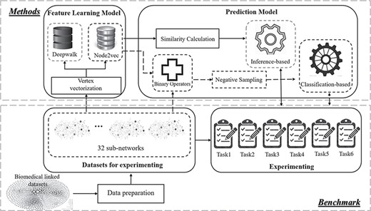
An overview of our network-based drug–target association prediction framework. The methods in the dotted box used in the comparison are detailed in the following sections.
Embedding-based feature learning
In order to train a model with the input network, we used the graph embedding method to learn the features of the nodes. Via graph embedding-based vectorization, nodes can be represented by a vector with a predefined length of dimension. Node2vec [30] is the state-of-art graph embedding method that vectorizes the vertices of a network based on the topology of the network with maximum likelihood optimization. Given a network |$G=\left(V,E\right)$|, Node2vec maximizes the probability of observing the neighborhood |$N(u)$| of each node |$u$| in the network based on two standard assumptions: (i) the likelihood of neighborhood observation is independent, and (ii) two nodes have a symmetric effect over each other for the conditional likelihood of source–neighborhood pair. For more details on Node2vec, please see Supplementary File 1. The vector formats of nodes will be used in the prediction component for the framework. For classification-based prediction, given the two vectors of a drug and target, the drug–target pair can be represented with a new vector-based on binary operators (Section 2.3.1). For inference-based prediction, the drug–drug/target–target similarity can be computed based on a cosine similarity with the two vectors (Section 2.3.2).
Association prediction
Classification-based prediction
Conventionally, the negative samples used in the classifier training are randomly selected from the huge number of unknown associations [4, 35]. Therefore, false positives in prediction can be predicted as the unknown positives but labeled as negative (i.e. false negatives) are used in training. We adapted a negative learning method, Spy, to select negative samples from the randomly selected unknown associations within certain confidence based on the expectation–maximization (EM) algorithm [35, 41]. |$s\%$| positive samples |$S$| serving as spies are randomly chosen to be removed from |$E$| and join |$U$| to form a mix set |$M$|. With |$M$| and |$P$| as the input, a classifier, I-EM, to classify |$M$| is obtained by training a Bayesian classifier to maximize the posterior probability of each document in |$P$|. with I-EM, all the samples that receive a classification score lower than |$t$| will be considered as negative, where |$t$| is determined by how the spy set |$S$| is classified with I-EM [41].
Statistics for the linked multipartite network (LMN)
| # Entity | Statistics | # Association | Statistics |
|---|---|---|---|
| Drug | 6990 | Drug–Target | 20 583 |
| Target | 4267 | Disease–Target | 13 205 |
| Disease | 3260 | Drug–Disease | 7232 |
| Side effect | 1695 | Drug–Drug | 38 140 |
| Pathway | 379 | Disease–Disease | 100 |
| Haplotype | 587 | Target–Target | 388 |
| Variant location | 2941 | Disease–haplotype | 3632 |
| In total | 20,119 | Drug–Haplotype | 3112 |
| Metrics | Statistics | Disease–Variant location | 12,277 |
| Average degree | 1.93E+01 | Drug–Variant location | 6868 |
| Average shortest path | 4.50E+00 | Disease–Pathway | 5057 |
| Average betweenness | 3.14E+04 | Drug–Pathway | 3889 |
| Average closeness | 4.50E+00 | Target–Pathway | 10 349 |
| Centralization (Evcent) | 9.80E−01 | Drug–Side effect | 69 464 |
| Density | 9.6 E−4 | In total | 194 296 |
Inference-based prediction
Two rule-based inference methods from our previous work [20], drug-based similarity inference (DBSI) and target-based similarity inference (TBSI), are adopted.
Benchmark
Dataset
This study incorporated information on the various biological entities related to drugs and their associated targets to form a linked multipartite network (LMN). The LMN is constituted of 12 repositories incorporating 20 119 entities and 194 296 associations covering 7 distinct entity types in total (see Table 1).
We extended the network presented in our previous study [20] with DrugBank version 4.1 and Bio2RDF release 3 [42] to build the backbone of the LMN, resulting in a network consisting of 6990 drugs, 4267 targets and 20 583 drug–target associations. We then augmented the network with supplementary information from four biological databases (human disease network [43], SIDER [44], KEGG [45] and PharmGKB [46]) as well as other cheminformatics resources (PubChem [47], UniProt [48], HGNC [49], OMIM [50], UMLS [51] and MESH [52]). For more details on the construction of this network, refer to Supplementary File 2. From this LMN, we produced 32 multipartite subnetworks with the differing combinations of entity types and their corresponding associations (see Supplementary Figure 1 for the graphical introduction and Supplementary Table 1 for statistics).
Experiment
There were two essentials critical to the adoption of the framework: (i) from a methodological perspective, how each component/method be coordinated in a favorable manner to achieve satisfactory prediction and (ii) from a data perspective, which network includes abundant biological entities and the corresponding relations that are preferable in prediction. Our benchmarking was thus conducted as a sequence of six distinct tasks detailed in the following.

Three types of node spaces in drug–target prediction tasks. The dark-grey ellipse and light-grey rectangle nodes are existent drugs and targets in a training bipartite network. Solid lines are the existent associations and dotted lines are the associations for prediction.
Task (1): Comparison of state-of-the-art network-based methods
A comparison to state-of-the-art network-based methods is conducted across four conventional experiments [12, 13], which predicts four types of targets: ‘enzyme’, ‘icon channel’, ‘nuclear receptor’, and ‘GPCR’. The drug–target associations in LMN are predicted based on the list of drugs and targets (271 drugs and 325 targets for enzyme, 129 drugs and 100 targets for ion channels, 48 drugs and 19 targets for nuclear receptors and 148 drugs and 77 targets for GPCR) obtained from http://web.kuicr.kyoto-u.ac.jp/supp/yoshi/drugtarget/ for four experiments, respectively. Six network-based methods, NRWRH [53], DTHybrid [23], NBI [14], RWR [53], DDR [2] and NTINet [21], are compared.
Task (2): Comparison of (semi-)classification-based, inference-based methods with the different feature generations
There are two components in the framework, feature generations and association prediction. For feature generation, DeepWalk and Node2vec were compared. For the prediction, inference-based methods (DBSI, TBSI and HBSI), classification-based methods (LR, SVM, RF and J48) and semi-classification-based methods (YASTI) were utilized separately in comparison. Four binary operations, Average, Hadamard, Weighted-L1 and Weighted-L2, are used alongside feature generation methods for classification- and semi-classification-based methods. Please note that our previously proposed methods are represented as DBSI+DeepWalk and TBSI+DeepWalk in this experiment as they were shown to be the best-performing in our previous study.
Task (3): effect of binary operators and classification methods
The proposed hybrid method constructs a prediction model as a combination of a classification and an inference model based on an embedding method for feature learning. We took all possible combinations of the factors, feature learning methods, binary operators and classification models, into consideration and study how these factors affect the results.
Task (4): negative samples for training and testing
The number of existent drug–target associations (i.e. positives) versus the number of nonexistent drug–target associations (i.e. negatives) is highly unbalanced, with the number of negatives significantly outnumbering the positives. To address this, all the positives were used whereas only a subset of the negatives was used in training and testing conventionally. As the nature of nodes in a pair-wise computation can have a significant impact on the results [27, 29], we want to investigate how well a drug–target association can be predicted with the incorporation of diverse types of negative associations. To distinguish the drug–target negatives in the data space (i.e. network), we classify the nodes into three kinds for each evaluation (see Figure 2), (i) Test Node Space (TNS), (ii) Connected Node Space (CNS) and (iii) All Node Space (ANS). We define TNS as the space that contains the drug and target nodes paired as positives for testing. CNS was defined as the space that contains the drug and target nodes having existent drug–target associations. ANS was defined as the space that contains all the drug and target nodes. Based on these three types of nodes, we can categorize all the negatives into seven types:
a) All Node Negatives (ANN), all possible negative pairs from the entire sets of drugs and targets.
b) Connected Node Negatives (CNN), negative pairs where both drug and target have at least one known drug–target association.
c) Test Node Negatives (TNN), a subset of CNN where both drug and target were used to form a positive pair in the test.
d) ANN-CNN, |$\left\{\left(d,t\right)|\left(d,t\right)\in ANN\wedge \left(d,t\right)\notin CNN\right\}$|.
e) ANN-TNN, |$\left\{\left(d,t\right)|\left(d,t\right)\in ANN\wedge \left(d,t\right)\notin TNN\right\}$|.
f) CNN-TNN, |$\left\{\left(d,t\right)|\left(d,t\right)\in CNN\wedge \left(d,t\right)\notin TNN\right\}$|.
g) ANN + TNN-CNN, |$\{\left(d,t\right)\mid \left(\left(d,t\right)\in ANN\vee \left(d,t\right)\in TNN\right)\wedge \left(d,t\right)\notin CNN$|}.
The AUC ROC score will be affected by the different types of negatives for both training and testing. Therefore, we randomly selected the negatives for each type for training and testing and studied the best strategy within 49 combinations in prediction.
Task (5): multipartite networks with differing combinations of entity types and their corresponding associations
To understand how the network constituted with a different combination of entity types will affect the prediction results, we utilized 32 subnetworks introduced in Section 3.1 to study.
Task (6): multipartite networks with different scales
To understand how networks with different scales affect prediction results, we generated the training networks with different scales by evenly removing the percentages of links ranging from 0.1 to 1.0. The 10 training networks are used to test the best-performing subnetworks that contain a differing number of entity types in Task (5).
Settings
We adopted a grid search strategy, which is a widely used strategy searching for hyperparameter optimization based on a specified subset of the whole hyperparameter space [54]. In our experiment, we carefully defined the range of each parameter by referencing the original settings presented in the articles relating to the methods adopted, as well as related drug–target prediction articles [20, 30, 31, 55]. Specifically, For Node2vec, the parameter ranges for the grid search specified as number of walks |$\gamma =\left\{10,40\right\}$|, Return |$p=\left\{0.5,1.0,2.0\right\}$|, in-out |$q=\left\{0.5,1.0,2.0\right\}$|, dimension |$d=\left\{64,128,256\right\}$|, window size |$w=\left\{5,10\right\}$|, walk length |$t=\left\{40,80\right\}$|. For DeepWalk, which was proved to be the best feature learning method for the similarity-based inference model in our previous work [20], the parameter ranges are specified as number of walks |$\gamma =\left\{10,40\right\}$|, learning rate |$\alpha =\left\{0.01,0.05,0.09\right\}$|, dimension |$d=\left\{\mathrm{64,128},256\right\}$|, window size |$w=\left\{5,10\right\}$|, walk length |$t=\left\{40,80\right\}$|. A detailed grid search for the proposed method refer to Supplementary Table 2.
For the classification-based model, we adopted four classification methods [2, 4, 30, 35], SVM, J48, RF and LR. The following settings are used for the classification methods, L2 regularization for LR, type C-SVC and kernel RBF for SVM, 500 trees for RF, confidence factor 0.25 for J48. Each drug–target pair was formalized using four binary operators, Average, Hadamard, Weighted-L1 and Weighted-L2. In addition, we adopted a semi-supervised classification method, YASTI, which used the unlabeled test data for training [36].
In practice, the LR classifier is obtained from the LIBLINEAR library (https://www.csie.ntu.edu.tw/~cjlin/liblinear/), J48 and RF are obtained from Weka library (https://www.cs.waikato.ac.nz/ml/weka/), SVM is obtained from LIBSVM (https://www.csie.ntu.edu.tw/~cjlin/libsvm/) and YASTI is obtained from collective library (https://github.com/fracpete/collective-classification-weka-package).
Validation and evaluation metrics
We used conventional 10-fold cross-validation for the evaluation, which randomly partitions the original samples into 10 equal-sized subsamples and conducted repeating independent experiments using each subsample for testing and the remaining 9 subsamples for training, repeating until each subsample has been used once for testing [5]. Since the inference-based methods required that all drugs and targets be connected in the network and could not predict the drug–target associations that contain the isolated drugs or targets, to fairly compare the proposed method to the existing methods, we limited the positives to the existent drug–target associations containing at least one un-isolated node. To achieve this, we first randomly extracted a set of existent drug–target associations |${E}_r$| from |$E$|, making sure that no isolated vertices of drugs and targets (e.g. a drug or a target has associated with at least one existent drug–target association) with the removing of |${E}_r$|. The remaining existent drug–target associations |${E}_c$| from |$E$| were used as base associations for training positives only. The associations |${E}_r$| were randomly partitioned into 10 subsets |$\left\{{E}_1,\dots .,{E}_{10}\right\}$| for 10-folder cross-validation. In each iteration (i.e. training and testing), a subset |${E}_i$|, was used as a gold standard for testing positives while the nine remaining subsets of |${E}_r$| as well as |${E}_c$| were used as the training positives. For the selection of negatives, different scenarios of negative generation from unknown drug–target associations |$U$| refer to Task (4) in Section 2.3.1.
We used the area under the receiver operating characteristic curve (AUC ROC) [56, 57], to assess the quality of the predictions. In practice, AUC ROC scores were calculated by the ROC JAVA library (https://github.com/kboyd/Roc) and Weka evaluation package [58]. In addition, Precision/Recall (PR AUC) is used to better illustrate the results for the highly imbalanced situations in the case study [59–61].
Results
Task (1): Comparison of state-of-the-art network-based methods
Table 2 shows that the proposed method significantly outperformed network-based methods in all four experiments (98.91% for enzyme, 99.28% for icon channel, 99.42% for nuclear receptor and 99.77% for GPCR). Even though NRWRH is the oldest method compared to other methods, it is the 2nd best-performing method. From the perspective of the target type, Icon channel achieved the best predictions (91.86%) compared to GPCR which achieved the worst predictions (81.15%) in an average.
Comparison of AUC scores (%) of network-based methods with four experiments
| Proposed | NRWRH | DTHybrid | NBI | RWR | DDR | NTINet | |
|---|---|---|---|---|---|---|---|
| Enzyme | 98.91 | 92.19 | 87.04 | 87.08 | 88.77 | 67.79 | 88.90 |
| Icon channel | 99.28 | 95.04 | 93.32 | 93.43 | 89.61 | 89.11 | 83.28 |
| Nuclear receptor | 99.42 | 80.22 | 80.33 | 80.49 | 71.31 | 73.02 | 83.28 |
| GPCR | 99.77 | 94.01 | 93.88 | 93.91 | 88.29 | 81.65 | 77.90 |
Underlined numbers represent best-performing scores
Task (2): comparison of (semi-)classification-based, inference-based methods with the different feature generations
Table 3 shows that the best result was achieved by the combination of classification and inference model based on Node2vec (AUC ROC: 95.3%). The best-performing solutions with a single prediction model are HBSI+Deepwalk (91.9%) and YASTI+SVM+Hadamard+Node2vec (93.1%). Our previous proposed inference-based prediction TBSI+Deepwalk still received a satisfactory result (91.66%).
Comparison of average AUC scores (%) of diverse predictions with different feature generation methods
| Prediction method | Feature generation | |||
|---|---|---|---|---|
| DeepWalk | Node2vec | |||
| Classification-based | LR | Average | 53.65 | 56.82 |
| Hadamard | 80.35 | 87.81 | ||
| Weighted-L1 | 74.49 | 85.90 | ||
| Weighted-L2 | 74.60 | 86.51 | ||
| SVM | Average | 62.20 | 83.30 | |
| Hadamard | 76.32 | 88.33 | ||
| Weighted-L1 | 75.26 | 86.59 | ||
| Weighted-L2 | 74.38 | 86.88 | ||
| RF | Average | 86.24 | 91.60 | |
| Hadamard | 89.60 | 93.00 | ||
| Weighted-L1 | 83.17 | 90.90 | ||
| Weighted-L2 | 83.19 | 90.91 | ||
| J48 | Average | 62.11 | 71.74 | |
| Hadamard | 67.09 | 73.50 | ||
| Weighted-L1 | 68.26 | 78.95 | ||
| Weighted-L2 | 68.56 | 77.44 | ||
| Semi-classification based (YASTI) | LR | Average | 81.59 | 89.68 |
| Hadamard | 86.45 | 92.86 | ||
| Weighted-L1 | 82.37 | 91.18 | ||
| Weighted-L2 | 81.65 | 90.80 | ||
| SVM | Average | 82.23 | 90.94 | |
| Hadamard | 86.34 | 93.11 | ||
| Weighted-L1 | 82.32 | 91.17 | ||
| Weighted-L2 | 81.63 | 90.79 | ||
| RF | Average | 82.31 | 90.40 | |
| Hadamard | 86.07 | 92.68 | ||
| Weighted-L1 | 82.37 | 91.21 | ||
| Weighted-L2 | 81.73 | 90.82 | ||
| J48 | Average | 82.68 | 90.36 | |
| Hadamard | 85.89 | 92.37 | ||
| Weighted-L1 | 82.42 | 91.20 | ||
| Weighted-L2 | 81.79 | 90.87 | ||
| Inference-based | DBSI | 88.79 | 89.54 | |
| TBSI | 91.66 | 85.25 | ||
| HBSI | 91.89 | 90.61 | ||
| Classification (SVM + average) + HBSI | 91.94 | 95.30 | ||
Table 3 also illustrates two phenomena: (i) the Node2vec-based methods show better results than DeepWalk-based (P = 8.18 E-05) for the combination model and a single classification model; (ii) the semi-classification-based methods outperform classification-based ones (P = 4.22 E-05) for the single classification model.
Task (3): effect of Binary operators and classification methods
Of the binary operators, Average performed the best (AUC ROC = 95.3%) and Hadamard performed the second (AUC ROC = 94.5%). Average performed the best for most of the cases except for the word2vec with semi-classification. Weighted-L1 and Weighted-L2 show similar results for all the tests.
Of the classification methods, SVM performed the best for Node2vec (AUC ROC = 95.3%), followed closely by RF which performed the second (AUC ROC = 94.9%). For semi-classification, only the vectorization methods were important, as can be seen by the similar AUC scores within DeepWalk and Node2vec groups.
In contrast to the single classification model, both Figure 3A and B illustrate that a classification-based solution outperformed the semi-classification-based solution (P = 0.013) for the combination model.
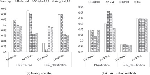
Comparison of methods for the two components in the proposed method. A Binary operator. B Classification methods.
Task (4): negative samples for training and testing
As shown in Table 4, the AUC ROC varies depending on the specific negative samples used for training and testing, and the best AUC ROC achieved using ANN-CNN for training and testing, which boasts a near 1.5% improvement compared with ANN-CNN+TNN in Task (3). Compared to the existent associations (i.e. positive samples) in TNN for training, ANN-CNN provides the most distinguishable negative samples, which gives the best classification results. Table 4 also gives the best training set for each kind of prediction test scenario, in which the best training negatives lay in the diagonal of the table.
AUC scores (%) of the prediction results of the proposed method with different combinations of training and testing negative samples
| Test negatives | ||||||||
|---|---|---|---|---|---|---|---|---|
| TNN | CNN-TNN | ANN-CNN | CNN | ANN-CNN + TNN | ANN-TNN | ANN | ||
| Train Negatives | TNN | 93.37 | 94.79 | 95.40 | 94.81 | 94.74 | 94.86 | 94.62 |
| CNN-TNN | 90.66 | 96.18 | 96.07 | 96.19 | 94.53 | 96.20 | 96.05 | |
| ANN-CNN | 91.19 | 96.00 | 96.79 | 95.95 | 95.18 | 96.00 | 95.82 | |
| CNN | 90.68 | 96.17 | 96.06 | 96.18 | 94.52 | 96.20 | 96.04 | |
| ANN-CNN + TNN | 91.73 | 95.87 | 96.57 | 95.89 | 95.16 | 95.91 | 95.71 | |
| ANN-TNN | 90.67 | 96.14 | 96.08 | 96.16 | 94.55 | 96.19 | 96.02 | |
Underlined numbers represent best-performing scores
Task (5): multipartite networks with a diffident combination of entity types and the corresponding associations
As shown in Table 5, the AUC scores generally improve as the number of entity types incorporated into the subnetworks increases. While the highest AUC was achieved using a Drug–Target–Pathway–Side effect–Variant location (D–T–P–S–V) network, the score was not much improved with the incorporation of additional entity types. We also studied that it is possible to obtain the highest AUC score with a greedy search by adding one specific type for the network with different types. As Supplementary Figure 2 shows, the best AUC score for the tri-partite network is D–T–P (AUC: 0.9571), that for quad-partite is D–T–P–S (AUC: 0.9568) and that for penta-partite is D–T–P–S–V (AUC: 0.9571). We also noticed that, despite identifying in our previous study [20] that using Drug–Target–Disease (D–T–I) would outperform the D–T networks, it is not the best option for prediction as a tripartite network.
AUC scores (%) of subnetworks with different shapes
| # Types | Network | AUCs | # Types | Networks | AUCs |
|---|---|---|---|---|---|
| 2 | D–T | 92.92 | 5 | D–T–P–S–V | 95.71 |
| 3 | D–T–V | 92.85 | 5 | D–T–P–H–V | 94.80 |
| 3 | D–T–I | 93.46 | 5 | D–T–P–I–S | 95.64 |
| 3 | D–T–H | 93.09 | 5 | D–T–P–S–H | 95.58 |
| 3 | D–T–S | 94.27 | 5 | D–T–I–S–V | 94.18 |
| 3 | D–T–P | 94.79 | 5 | D–T–I–S–H | 94.30 |
| 4 | D–T–P–V | 94.73 | 5 | D–T–I–H–V | 93.56 |
| 4 | D–T–I–S | 94.40 | 5 | D–T–P–I–H | 95.18 |
| 4 | D–T–P–I | 95.10 | 5 | D–T–P–I–V | 94.82 |
| 4 | D–T–P–S | 95.68 | 5 | D–T–S–H–V | 94.27 |
| 4 | D–T–S–H | 94.44 | 6 | D–T–P–I–H–V | 95.03 |
| 4 | D–T–I–H | 93.62 | 6 | D–T–P–I–S–V | 95.50 |
| 4 | D–T–P–H | 94.84 | 6 | D–T–I–S–H–V | 94.24 |
| 4 | D–T–H–V | 92.79 | 6 | D–T–P–S–H–V | 95.59 |
| 4 | D–T–I–V | 93.63 | 6 | D–T–P–I–S–H | 95.50 |
| 4 | D–T–S–V | 94.23 | 7 | D–T–P–I–S–H–V | 95.33 |
Underlined numbers represent best-performing scores
Task (6): multipartite networks with different scale
Figure 4 shows that, for all the best-performing subnetworks, AUC scores were inversely proportional to the number of links removed in training. In other words, larger training networks had better prediction capabilities. For example, the best-performing network D–T–P–S–V improved the prediction from AUC: 0.9292 to AUC: 0.9571 by increasing the relative number of links to 100%.
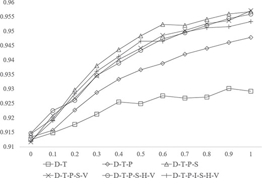
AUC scores of best subnetworks in different shapes with different scales.
Results from Tasks 5–6 illustrate two important findings for network-based prediction, (i) with respect to the components in the network, adding entities in different types and the corresponding links will not always lead to a prediction performance improvement. Our experiment shows that the readers have to be careful about what entities are integrated and how to sample the corresponding associations in training; (ii) with respect to the scale of the network, adding more entities of the same types and the corresponding links will improve the prediction. The best strategy to improve the prediction performance of network-based methods is therefore to update the network with more databases consisting of entities and links of the same type used in the original network rather than integrating more related databases with new types of entities and links.
A case study based on external validation
As a case study, we show the reliability of the predictions based on an external validation using novel drug–target associations. In practice, we searched DrugBank version 5.1.0 and identified 75 novel drug–target associations for 20 diseases as the positives to test the proposed framework. For negatives, we randomly selected |$\mathrm{k}\times r$| negatives for each negative types introduced in Task 4 for each disease with |$k$| positive associations, where |$r$| is the skew ratio [60] ranging from |$[10,50,100,500,1000]$| as the negatives outnumber positives in the real screening stage. In total, there are around 450 000 associations for testing (see Supplementary Figure 3 for the graphical introduction of the predictions in detail). We trained our model with the entire LMN with the best-performing parameter setting.
As Table 6 shows, the best AUC ROC scores were obtained for ‘Adenocarcinoma’, ‘Anemia’, ‘Apert syndrome’, ‘Autism’, ‘Cirrhosis’, ‘Galactosemia’, ‘Insomnia’, ‘Lung Cancer’, ‘Malaria’, ‘Obesity’, ‘Obsessive-Compulsive Disorder’ and ‘Spinal Muscular Atrophy’ (AUC ROC = 100%, PR AUC = 100%). Other diseases received AUC ROC scores ranging from 97.82 to 80.36%. The worst prediction was for ‘Macular Degeneration’ (PR AUC ROC = 0.09%). All the prediction for |$r$| ranging from |$[10,50,100,500,1000]$| refers to Supplementary Table 3.
Disease specific drug–target prediction with |$r=1000$|.
| ID | Disease | # Positives | AUC ROC | PR AUC |
|---|---|---|---|---|
| 1 | Adenocarcinoma | 1 | 100.00 | 100.00 |
| 2 | Anemia | 1 | 100.00 | 100.00 |
| 3 | Apert syndrome | 1 | 100.00 | 100.00 |
| 4 | Autism | 1 | 100.00 | 100.00 |
| 5 | Cirrhosis | 1 | 100.00 | 100.00 |
| 6 | Galactosemia | 1 | 100.00 | 100.00 |
| 7 | Insomnia | 1 | 100.00 | 100.00 |
| 8 | Lung cancer | 1 | 100.00 | 100.00 |
| 9 | Malaria | 1 | 100.00 | 100.00 |
| 10 | Obesity | 1 | 100.00 | 100.00 |
| 11 | Obsessive compulsive disorder | 4 | 100.00 | 100.00 |
| 12 | Spinal muscular atrophy | 1 | 100.00 | 100.00 |
| 13 | Stroke | 4 | 97.82 | 75.04 |
| 14 | Bipolar disorder | 3 | 96.99 | 66.72 |
| 15 | Asthma | 11 | 96.03 | 13.99 |
| 16 | Adrenal hyperplasia, congenital | 2 | 95.55 | 50.07 |
| 17 | Adrenal hyperplasia, congenital, due to 21-hydroxylase deficiency | 2 | 95.55 | 50.07 |
| 18 | Macular degeneration | 13 | 91.22 | 0.09 |
| 19 | Hypertension | 1 | 90.93 | 15.75 |
| 20 | Dementia | 24 | 80.36 | 22.33 |
| Total | 75 | 97.22 (average) | 74.70 (average) | |
In addition, we identified the top K predictions from the proposed method and calculated the percentage of positives predicted (i.e. Recall). Fifty associations are predicted over 75 positives (average 81.2% recall for each disease) with top 0.1% predictions (see Supplementary Figure 4). The summary and detail information of top K arranged from 0.01 to 1% for each disease can be found in Supplementary Tables 4 and 5.
The most prevalent predictions were found under asthma, hypertension and dementia diseases. Within these predictions, we have identified that through our model, we can locate reliable targets that can establish the most prevalent predictions. Our model highlighted several targets, including muscarinic acetylcholine receptor M2 in the asthma model, the alpha and beta-3 adrenergic receptors in the hypertension model and the pregnane X receptor (PXR) in the dementia model, for further studies.
These targets possessed one of the highest numbers of associations and have resulted in the highest amount of successful predictions compared to the rest of the model. In addition, they were closely related to the physiological effects of these particular diseases. For example, muscarinic acetylcholine receptor M2 serves as a binding site for agonists in order to potentially alleviate the symptoms of asthma. Likewise, the targets, alpha and beta-3 adrenergic receptors and PXR, found in hypertension and dementia model respectively also presented similar biological significances.
Additionally, the results also emphasized the relationship they have with other targets or nodes. For example, in the hypertension model, the targets were able to show that the drug relations with the adrenergic receptors can be important in predicting new potential targets used for further drug developments for hypertension. Therefore, our model was able to highlight the potentials of these targets for future drug predictions due to their biological significance and the success with the drugs that currently use them as their targets. The detailed discussion of the three diseases refers to Supplementary File 3.
Discussion and conclusion
We have benchmarked various strategies as determined from a review process for constructing a network-based prediction framework that utilizes topological features of the network for prediction. We conducted this review and benchmarking from both a network and a methodological perspective. For data, (i) 32 distinct permutations of subnetwork arrangements were benchmarked, and (ii) a combination of off-the-shelf classification, inference and graph embedding methods were reviewed. Benchmarking was used to determine the best-performing strategies from both network and methodological perspectives. With a case study based on prediction for a distinct set of 20 diseases, we demonstrated the validity of the framework constructed from the methodologies that were identified to be best-performing to identify novel drug–target associations.
The main advantage of the presented framework is to enable the modularization of prediction. Thus, the diverse methods, such as graph embedding and classification/Deep Learning methods [62–64], can be easily adapted in feature learning and association prediction components, which provide a flexible and extendable solution in a long run. To tackle isolated drugs/targets which cannot be embedded in our current solution, the inference and classification methods are further facilitated with two interfaces (refer to Supplementary Figure 5). With such a mechanism designed in the proposed framework, predictions can be made based on the similarity matrices, such as similarities based on drug classification systems [26], chemical structure/genomic sequence and pharmacology [19]. More specifically, drug–drug and target–target similarities can be directly fed to an inference model, and a vectoral representation based on the existing embedding of the similar drugs/targets can be generated for classification. Last but not least, in addition to the benchmarking and framework, we provide the indispensable resources, a runnable open source.
(https://github.com/zongnansu1982/Prediction_Basedon_Biolinkednetwork_Mining) and a web-based drug–target prediction application (https://zongnansu1982.shinyapps.io/drug_target_prediction_demo_20190427/). The resources/tools and results of the reviewed networks and models based on off-the-shelf methods are presented in a way that can be adapted as a well-documented baseline for future network-based studies. Three applications of this work can be summarized as follows: (i) with the runnable tools developed, drug–target prediction can be achieved to support drug repurposing; (ii) with the extendable framework proposed, new solutions can be developed based on the adaption of new algorithms for the existing components; and (iii) newly developed computational methods can be evaluated with the proposed benchmark and compared to the proposed framework.
Despite the reliability of the network-based framework proven in this study, there are a few issues that can be addressed in the future.
Firstly, the graph embedding method for feature learning can be improved. Biomedical linked datasets and real-world heterogeneous networks contain diverse properties to describe the knowledge and data, while their associations are equally considered and are computationally indistinguishable for embedding, which loses a large amount of information for prediction. Even a straightforward solution is to apply multidimensional weighted graphs; to the best knowledge for the authors, there is a lack of a solid embedding solution for multidimensional weighted graphs and it is not feasible to weight the properties. A simpler solution is to embed multidimensional graphs [65, 66]. Instead of integrating heterogeneous networks to obtain a network for feature learning, vector fusion methods can be applied to formalize a node vector based on the vectors learned from each heterogeneous network [21].
Secondly, feature learning and classification are sequentially combined in classification-based drug–target prediction models [30, 31, 55]. Feature learning plays an important role by directly affecting the final classification results, but the same does not hold true in reverse. It is therefore desirable that feature learning methods would allow dynamic tuning based on cross-validation on the follow-up classification model, which may improve predictive performance. One potential solution is to adopt deep neural networks to connect feature learning and classification together in a prediction model and provide an implicit feedback mechanism for updating these parameter values [67]. While such methods will sacrifice flexibility and re-usability, it might be interesting to study which solution fits the practical scenarios better.
Lastly, one of the main objectives for the computational drug–target prediction methods is to narrow down the screening candidate for in vitro experiments, such as drug-repurposing. Therefore, in practical applications, with a list of given drugs or targets as the input, the whole targets or drugs in the database should be considered as the potential candidate in prediction. The imbalanced test data in pairwise prediction will cause bias in the end result. Although we have discussed a strategy to select the negative pairs in training and testing to receive ideal AUC ROC scores, we did not give an efficient strategy to select test pairs that are most likely to be positives from the huge number of imbalanced candidates. Unlike with the negative selection method, we applied to find the most possible negatives [41]; the test sample search method would be to generate the most possible positive pairs based on the inputs. The endeavor to develop such an efficient search function (e.g. as a ranking function) to preselect the candidate test pairs (e.g. based on similarity) will advance the usage of the computational drug purposing methods.
While networks appear to be valuable and utilized in a diverse set of methods for prediction tasks, these networks cannot be reused and adapted for existing machine learning-based frameworks, where feature learning and prediction methods are modularized, which drives a necessity to investigate heterogeneous biomedical linked networks, as well as off-the-shelf methods, to enable such network-based frameworks.
We conducted a review and benchmarked the associated performance of combinatorial networks and methodologies for creating and mining associations from network-based representations of biomedical knowledge.
Our benchmarking strategy consisted of two series of experiments, totaling five distinct tasks, to test the performance of the different strategies from both network and methodological perspectives, and determine the best prediction.
The results of our benchmarking produced knowledge on a network-based prediction framework with the modularization of the feature selection and association prediction, which can be easily adapted and extended to other feature sources or machine learning algorithms as well as performed baseline to comprehensively evaluate the utility of incorporating varying data sources.
Acknowledgements
The authors appreciate the valuable opinion and editing from Dr Hyeoneui Kim and Dr Hongfang Liu. The authors also thank Dr Sejin Nam and Dr Victoria Ngo for providing support on the computation and proofreading.
Dr Nansu Zong is a Researcher Associate at the Department of Health Sciences Research, Mayo Clinic. His research focuses on the development of Deep Learning methods and biological databases for drug re-purposing.
Mayo Clinic is a charitable, nonprofit academic medical center that provides comprehensive patient care, education in clinical medicine and medical sciences and extensive programs in research. Dr Nansu Zong is a member of the Department of Health Sciences Research, which is a multidisciplinary group of approximately 90 doctoral-level and more than 400 allied health staff members, located in Phoenix/Scottsdale, Arizona; Jacksonville, Florida; and Rochester, Minnesota.
Footnotes
DrugBank, Human Disease Network, Sider, KEGG, PharmGKB, PubChem, OMIM, UniProt, HGNC, UMLS, MESH, Bio2RDF
Drug, target, disease, Sider effect, pathway, haplotype, variant location
(i) Adenocarcinoma, (ii) anemia, (iii) Apert syndrome, (iv) autism, (v) cirrhosis, (vi) galactosemia, (vii) insomnia, (viii) lung cancer, (ix) malaria, (x) obesity, (xi) obsessive compulsive disorder, (xii) spinal muscular atrophy, (xiii) stroke, (xiv) bipolar disorder, (xv) asthma, (xvi) adrenal hyperplasia, congenital, (xvii) adrenal hyperplasia, congenital, due to 21-hydroxylase deficiency, (xviii) macular degeneration, (xixx) hypertension, (xx) Dementia
Availability: The proposed method is available, along with the data and source code at the following URL: https://github.com/zongnansu1982/Prediction_Basedon_Biolinkednetwork_Mining. The web application can be found at https://zongnansu1982.shinyapps.io/drug_target_prediction_demo_20190427/.
Contact: [email protected].
