


Abstract
Label-free quantification (LFQ) with a specific and sequentially integrated workflow of acquisition technique, quantification tool and processing method has emerged as the popular technique employed in metaproteomic research to provide a comprehensive landscape of the adaptive response of microbes to external stimuli and their interactions with other organisms or host cells. The performance of a specific LFQ workflow is highly dependent on the studied data. Hence, it is essential to discover the most appropriate one for a specific data set. However, it is challenging to perform such discovery due to the large number of possible workflows and the multifaceted nature of the evaluation criteria. Herein, a web server ANPELA (https://idrblab.org/anpela/) was developed and validated as the first tool enabling performance assessment of whole LFQ workflow (collective assessment by five well-established criteria with distinct underlying theories), and it enabled the identification of the optimal LFQ workflow(s) by a comprehensive performance ranking. ANPELA not only automatically detects the diverse formats of data generated by all quantification tools but also provides the most complete set of processing methods among the available web servers and stand-alone tools. Systematic validation using metaproteomic benchmarks revealed ANPELA’s capabilities in 1 discovering well-performing workflow(s), (2) enabling assessment from multiple perspectives and (3) validating LFQ accuracy using spiked proteins. ANPELA has a unique ability to evaluate the performance of whole LFQ workflow and enables the discovery of the optimal LFQs by the comprehensive performance ranking of all 560 workflows. Therefore, it has great potential for applications in metaproteomic and other studies requiring LFQ techniques, as many features are shared among proteomic studies.
Introduction
Microbial community (MC) is characterized by widely diverse species and highly dynamic compositions [1, 2] that make it closely associated with the pathogenesis of various diseases (such as cancer [3], inflammatory disease [4] and metabolic disorder [5]), the productivity of agricultural plants [6, 7], the biogeochemical cycle of complex environmental matrices [8, 9] and so on. Investigations of the protein abundance in specific MC have enabled an unprecedented view of the adaptive response of microbes to external stimuli or their interaction with other organisms or host cells [10, 11]. Due to its superior ability to provide quantitative and dynamic information on microbiome’s functional activity by directly profiling protein expression [12], metaproteomics stands out from other OMIC (any research field of biological study ending in -omics such as genomics, proteomics or metabolomics) techniques and becomes popular in current MC studies [13–18]. Thus far, several methods have been developed to quantify metaproteomic data [19]. Due to the simplicity of its experimental design and its ability to process large sample cohorts [20], label-free quantification (LFQ) is the most widely employed approach able to monitor the intestinal responses to gut microbiota [21–23], decipher the diversity and dynamics of bacterial proteome [24], reveal the abnormal abundance of proteins [25] and so on.
However, the low precision [26], poor reproducibility [27, 28], inaccuracy [29] and false discovery rate [30, 31] of the LFQ of microbial proteins have emerged as the key ‘technical challenges’ in recent metaproteomic study [27–29, 32–35]. These challenges may be attributed to (1) heterogeneity among microbial samples [36], (2) vast dynamic range of protein abundance [29], (3) highly random nature of experimental sampling [32], (4) systematic variations among sample preparations or experimental runs [12, 26, 32] and (5) enlarged search space in metaproteomic study [2, 30, 31]. The substantial variations in microbial signaling or phenotypes are frequently reported to originate from subtle changes in microbial samples [37–39], but these changes are rarely detected if an LFQ does not perform well [27]. Thus, a variety of acquisition techniques [40, 41], quantification tools [41, 42] and subsequent processing methods (transformation, normalization, missing value filtering and imputation) [43, 44] have been developed and extensively used to increase precision, enhance reproducibility and improve accuracy of LFQ in current proteomic studies (Supplementary Table S1).
Till now, 3 acquisition techniques (2 modes of acquisition), ≥18 quantification tools (Table 1) and dozens of subsequent processing methods (≥4 transformation, ≥16 normalization and ≥ 8 filtering/imputation) have been sequentially integrated to form numerous LFQ workflows. As reported, different LFQ workflows can produce considerably different or, in some cases, contradictory results [45], and the suitability of a specific workflow depends heavily on the particular data set analyzed [46]. It is now of great interest to compare the performances among various quantification tools [20, 33] and different label-free techniques [47, 48], and the selection of the optimal workflow for a specific data set is urgently needed [49], which is however a very challenging task in metaproteomics. First, the feasibility of discovering the optimal LFQ workflow is severely hampered by the huge number of possible combinations. Taking the subsequent processing methods as example, there are over 500 possible combinations of transformation, normalization and filtering/imputation approaches. Second, the criterion used to assess LFQ’s performances is critical but also a great challenge for selecting the optimal workflow [40, 50]. LFQ’s performance is primarily evaluated by ‘precision’ (intragroup variations) [50], but a variety of new criteria could also be applied [20, 51, 52]. As these criteria complement one another, it is highly recommended to collectively employ these criteria as a ‘thorough’ evaluation of each workflow [46, 47, 52].
Several powerful LFQ-related tools (Supplementary Table S2) are currently available [53–58]. Perseus [53] and Gmine [54] integrate various processing methods in their corresponding analysis chain, but no assessment on the performances of LFQ is conducted. ‘LFQbench’ [20] and ‘msCompare’ [55] are recognized as evaluating the performances of 3~5 quantification tools [20, 55], and ‘Normalyzer’ [56], ‘SPANS’ [57] and ‘GiaPronto’ [58] are distinguished for being able to assess 1~8 normalization methods [56–58]. Since a typical LFQ workflow integrates both quantification tools and processing methods, any assessment focusing solely on the tool or the method could not fully reflect the overall performance of the whole workflow. Moreover, none of the available tools could systematically evaluate the performance, as highly recommended by previous studies [46, 47, 52], based on all those proposed criteria (each with distinct underlying theory) [20, 47, 59–63], and it is impossible for these tools to discover the workflows of optimal performance by comprehensively ranking all (more than 500) possible quantification combinations. Thus, it is essential to develop new tools to assess the performance of the whole LFQ workflow from multiple perspectives and identify the optimal one based on comprehensive performance ranking.
Herein, an open access server ANPELA was constructed and validated to enable the performance assessment of whole LFQ workflow (18 quantification tools accompanied by the combination of 28 processing methods). Five well-established criteria [20, 59–63] were collectively used for the first time to facilitate comprehensive assessment from multiple perspectives. ANPELA not only automatically detects the diverse formats of data generated by all quantification tools but also comprehensively provides the most complete set of processing methods among the available web servers or stand-alone applications. Moreover, it enables the identification of the optimal LFQ workflow(s) based on a comprehensive performance ranking. To validate its ability to (1) discover well-performing workflow(s), (2) enable assessment from multiple perspectives and (3) validate LFQ accuracy using spiked proteins, 16 benchmark data sets were collected and 4 independent metaproteomic cases were studied. In conclusion, ANPELA is unique for its ability to evaluate the performance of the whole LFQ workflow and enable the discovery of the optimal one(s) by comprehensive performance ranking, which can thus greatly facilitate proteome quantification for current metaproteomic research.
Materials and methods
Quantification tools and subsequent processing methods used in ANPELA
Eighteen quantification tools for preprocessing mass spectrometry (MS)-based raw data acquired by three acquisition techniques (Peak intensity, Spectral counting and SWATH-MS) were provided in ANPELA (Supplementary Method S1), which included Abacus [64], Census [65], DIA-Umpire [66], DTASelect [67], IRMa-hEIDI [68], MFPaQ [68], MaxQuant [69], OpenMS [70], OpenSWATH [20], PEAKS [71], ProteinProphet [72], Proteios SE [73], Progenesis [44], SWATH 2.0 [20], Skyline [74], Spectronaut [75], Scaffold [33] and Thermo Proteome Discoverer [33]. Moreover, 28 subsequent processing methods were used for analyzing metaproteomic data (Supplementary Method S2), which included 4 transformation (Box–cox [76], Cube root [77], Log transform [78] and Power [79]), 16 normalization (Auto Scaling [80], Cyclic Loess [81], EigenMS [50], Linear Baseline Scaling [82], Lowess [83], Median [84], Mean [85], Median Deviation [86], Pareto Scaling [87], PQN [88], Quantile [82], Robust Linear Regression [50], TIC [89], TMM [90], VSN [91] and Z-score [92]) and 8 filtering or imputation (Back [44], Basic [44], Bpca [44], Censor [44], Knn [93], Lls [44], Svd [93] and Zero [94]). To make the discussion in this study clearly understood, a three-letter abbreviation was assigned to each method (Table 2), and the brief descriptions of these methods were also provided in Table 2.
Overview on 18 quantification tools together with their corresponding mode of acquisition, acquisition technique and quantification metric. APEX, absolute protein expression index; Average-Top3, average intensity of the three highest intense peptides; emPAI, exponentially modified protein abundance index; iBAQ, intensity-based absolute quantification; IRP, internal reference peptide; MaxLFQ, delayed normalization and maximal peptide ratio extraction; NoC, intensity of nonconflicting peptides; NSAF, normalized spectral abundance factors; PAI, protein abundance index; Raw, raw spectral counts; Summed-Top3, summed intensity of the three highest intense peptides; TIC, total ion current; TPA, total protein approach; TRIC, transfer of identification confidence
| Mode ofacquisition | Acquisition technique | Representativequantification tools | Quantification metric provided |
|---|---|---|---|
| Data-dependent acquisition (DDA) | Spectral counts (MS2) | Abacus | NSAF [47, 64, 130] |
| Census | Raw [65] | ||
| DTASelect | Raw [67] | ||
| IRMa-hEIDI | Raw [129] | ||
| MaxQuant | emPAI; APEX [47, 69, 130] | ||
| MFPaQ | PAI [131] | ||
| ProteinProphet | Raw [132] | ||
| Thermo Proteome Discoverer | NSAF [33, 47, 130] | ||
| Scaffold | emPAI; NSAF; Total spectra; Weighted spectra [133] | ||
| Peak intensity (MS1) | MaxQuant | MaxLFQ; Summed-Top3; iBAQ; TPA [69] | |
| MFPaQ | TIC; Average TIC [134] | ||
| OpenMS | TIC; Top three TIC [135] | ||
| PEAKS | Average-Top3; Summed-Top3 [136] | ||
| Progenesis | Average-Top3; NoC [33, 137] | ||
| Proteios SE | Summed-Top3 [48,73] | ||
| Scaffold | Average-Top3; iBAQ; TIC [138] | ||
| Skyline | Average-Top3 [139] | ||
| Thermo Proteome Discoverer | Minora algorithm [140, 141] | ||
| Census | Weighted overall intensities [142] | ||
| Data-independent acquisition (DIA) | SWATH-MS | DIA-Umpire | Data-centric iBAQ abundance measures and ‘Top N’ metrics [65] |
| OpenSWATH | Peptide-centric TRIC algorithm [143, 144] | ||
| PeakView | Peptide-centric extracted ion chromatograms alignment [145] | ||
| Spectronaut | Peptide-centric ‘target-decoy’ search strategy [75] | ||
| Skyline | Peptide-centric IRP method [146] |
Abbreviated names of the subsequent processing methods used in this study together with their corresponding full names and brief descriptions
| Processing method (abbreviation) | Brief description of each method | |
|---|---|---|
| Transformation | Box–Cox Transformation (BOX) | Transforming data based on linearity, normality and homoscedasticity assumption [76] |
| Cube Root Transformation (CUB) | Improving normality distribution of simple count data [77] | |
| Log Transformation (LOG) | Almost routinely carried out for reaching a more symmetricdistribution [78] | |
| None (NON) | No transformation method applied | |
| Power Transformation (POW) | Stabilizing variance and making data more normal distribution-like [79] | |
| Normalization | Auto Scaling (ATO) | Scaling protein intensities based on the standard deviation of OMICdata [80] |
| Cyclic Loess (CYC) | Estimating a regression surface using multivariate smoothingprocedure [81] | |
| EigenMS (EIG) | Preserving true differences based on treatment effect and singularvalue decomposition [50] | |
| Linear Baseline Scaling (LIN) | Mapping each spectrum to the baseline based on a constant linearrelationship [82] | |
| Locally Weighted Scatterplot Smoothing (LOW) | Normalizing a proteomic data set by compensating for non-linearbias [83] | |
| Mean Normalization (MEA) | Normalizing the data by mean value of all signals to eliminatebackground effect [84] | |
| Median Absolute Deviation (MAD) | A measure of the spread of the data and used to estimate the samplestandard deviation [85] | |
| Median Normalization (MED) | Scaling the samples so that they have the same median [86] | |
| None (NON) | No normalization method applied | |
| Pareto Scaling (PAR) | Reducing the weight of large fold changes in protein intensities bystandard deviation [87] | |
| Probabilistic Quotient Normalization (PQN) | Transforming the spectra based on an overall estimation on the mostprobable dilution [88] | |
| Quantile Normalization (QUA) | Achieving the same distribution of protein intensities across allsamples [82] | |
| Robust Linear Regression (RLR) | Used for transference to rescale one reference interval to anotherscale [50] | |
| Total Ion Current (TIC) | Summing all the separate ion currents carried by the ions of differentm/z [89] | |
| Trimmed Mean of M Values (TMM) | Estimating scale factors between samples for differential expressionanalysis [90] | |
| Variance Stabilization Normalization (VSN) | A non-linear method for keeping the variance constant over the entiredata range [50] | |
| Z-score normalization (ZSC) | Normalizing data based on the mean and standard deviation [92] | |
| Imputation | Background Imputation (BAK) | Simulating the situation where protein values are missing [44] |
| Bayesian Principal Component Imputation (BPC) | Providing capacity to auto-select the parameters used in theestimation [44] | |
| Censored Imputation (CEN) | Imputing non-missing completely at random missing values by lowestintensity value [44] | |
| K-nearest Neighbor Imputation (KNN) | Imputing values based on K proteins similar to the proteins withmissing values [93] | |
| Local Least Squares Imputation (LLS) | Missing value imputation by a linear combination of similar genesidentified by KNN [44] | |
| None (NON) | No imputation/filtering method applied | |
| Singular Value Decomposition (SVD) | Estimating the missing values based on a linear consideration [93] | |
| Zero Imputation (ZER) | Replacing the missing values with zeros deemed to the simplestimputation method [94] |
Criteria and corresponding assessment metrics for evaluating the performance of LFQ workflow
Besides the criterion ‘precision’ (intragroup variations) primarily applied for assessing the performance of LFQ [50], a variety of criteria have been developed and applied in the LFQ-related studies [20, 51, 52]. Due to the independent nature of these criteria [47], they are known to complement one another and highly recommended to be collectively employed for ‘thoroughly’ evaluating specific LFQ workflow [46, 47, 52]. Particularly, two independent criteria, ‘precision’ and ‘accuracy’, were collectively considered to enable the in-depth evaluation of LFQ [20, 44, 50], and three independent criteria were further integrated for the first time to comparatively evaluate various LFQ methods [47]. Moreover, an appropriate LFQ is expected to retain or even increase the difference in proteomic data between two distinct sample classes [59, 95]. In the meantime, the reproducibility of identified markers is also recognized as another independent criterion for assessing the performance of LFQ [52]. Thus, five independent criteria were used here to assess the performance of an LFQ workflow in ANPELA (each measured by a variety of assessment metrics; Supplementary Method S3).
(a) Precision of LFQ based on the proteomes among replicates
Different acquisition techniques, various tools for preprocessing raw proteomics data and diverse approaches for data processing (transformation, normalization, filtering and missing value imputation) could profoundly affect the precision of LFQ [20], which was assessed by pooled coefficient of variation (PCV) of the reported protein intensities among replicates [20, 96]. PCV was thus adopted as an assessment metric reflecting LFQ’s ability to reduce variations among replicates [97] and to enhance technical reproducibility [56]. A lower value of PCV indicates a more complete reduction of unwanted signals (denoting improved LFQ precision) [98].
(b) Classification ability of LFQ between distinct sample groups
An appropriate LFQ is expected to retain or even increase the difference in metaproteomic data between two distinct sample groups [59, 95]. Two-way clustering of proteins identified from these two groups is thus used as an assessment metric to assess LFQ classification ability [95, 99]. First, the total number of protein intensities in each sample is reduced by feature selection. Then proteins (rows) and samples (columns) are clustered by their similarities in a protein intensity profile. Details can be found in Supplementary Method S3.
(c) Differential expression analysis based on reproducibility optimization
To avoid overfitting/confounding in LFQ, distribution of P-values of protein intensities between two distinct sample groups is examined [100, 101]. Unbiased variation is expected for the majority of proteins (without clear differentiation of expression), with an obvious peak in the [0.00, 0.05] interval corresponding to proteins with differential intensities [101]. Moreover, a volcano plot of proteins with differential intensity provides a glimpse of the total number of differentially expressed proteins [102]. In a metaproteomic study exploring mechanisms underlying complex biological process, the limited number of differentially expressed proteins may result in false discovery [103]. Thus, the statistical differences (P-value) of protein intensities between distinct groups are first estimated by reproducibility-optimized test statistic (ROTS) [61, 104]. Distribution of P-values is then provided, and a skewed distribution may indicate overfitting and/or confounding [105].
(d) Reproducibility of the identified protein markers among different data sets
Consistency score (CS) is a popular assessment metric representing the reproducibility of identified markers [52, 106] and is used to assess the level of consistency among the protein markers discovered from the various portions of a given data set [107]. A higher CS denotes a more stable discovery of markers [52]. First, a random sampling is conducted on the studied data set to generate multiple sub-data sets. Then each protein is ranked based on its significance (q-value) and absolute fold change. Finally, those top-ranked proteins in each sub-data set are selected as markers before the calculation of the CS (Supplementary Method S3).
(e) Accuracy of LFQ based on spiked and background proteins
Extra experimental data (e.g. spiked proteins) are frequently generated and used as a reference to validate or adjust LFQ’s performances [20, 96], and it is therefore straightforward to know the expected log fold changes (logFCs) for both spiked and background proteins (the expected logFC for background proteins is zero) [102]. First, the differentially expressed proteins are identified by ROTS. Then the true positive rate (TPR) for the successful discovery of spiked protein is calculated. A higher TPR corresponds to a greater accuracy. Moreover, the logFCs of protein intensity (for both spiked and background proteins) between distinct sample groups are measured, and the correlation between measured and expected logFCs is then assessed by mean squared error. A higher level of correlation indicates a more accurate LFQ workflow [102].
Each criterion above evaluated the LFQ performance based on its own underlying theory, and the combination of multiple criteria resulted in a systematic assessment. The assessment results are directly provided as tables or illustrated as plots online, all of which can be downloaded from the ANPELA web page. More information can be found in Supplementary Method S3.
Details of web server implementation
Official (https://idrblab.org/anpela/) and mirror (http://idrb.zju.edu.cn/anpela/) sites of ANPELA are deployed on a server running ‘Cent OS Linux v7.0 operating system’, ‘Apache HTTP web server v2.2.15’ and ‘Apache Tomcat servlet container’ (http://httpd.apache.org). The web interface was constructed by R Package v3.4.1 (Shiny v0.13.1) running on the Shiny-server v1.4.1.759 (http://www.rstudio.com/shiny). A number of R packages were utilized in the background processes including affy, AUC, DiffCorr, DT, e1071, fastlo, ggfortify, ggsci, ggplot2, gplots, impute, limma, LPE, metabolomics, MetNorm, NOISeq, pcaMethods, png, RcmdrMisc, ROTS, rmarkdown, ropls, shiny, shinyBS, shinydashboard, shinyRGL, statTarget and vsn. ANPELA website can be readily accessed by all users with no login requirement and by a variety of popular web browsers including Google Chrome, Mozilla Firefox, Safari and Internet Explorer (10 or later). For using the stand-alone version of ANPELA downloaded directly from the official and mirror sites, the installation of R environment is required before its running. The ‘User Manual’ of the stand-alone version of tool was provided in Supplementary Method S4.
The input formats required by ANPELA
The input files required by ANPELA are the standard output raw files of the 18 quantification tools, together with a label file indicating the category of each sample. The standard output raw files of quantification tools are described in the ‘Tutorial’ panel of ANPELA. Alternatively, a standard format designed by ANPELA is also accepted for assessing the in-house tool or predefined analytical workflow, which should be in ‘csv’ format with the dimension of m × n (m and n indicate the numbers of metaproteomic features and microbial samples, respectively). Additionally, an additional file providing the concentrations of known proteins (such as spiked proteins) is required to assess the performances of LFQ based on the last criterion. Specifically, the extra file should contain the ‘class of samples’ and the ‘Sample ID’. The ‘Sample ID’ should be unique and defined by the preference of the ANPELA user, and the ‘class of samples’ refers to the group of ‘Sample ID’. The input sample file can be found in the ‘Tutorial’ panel of ANPELA.
The formats and visualization of ANPELA output files
The output files of ANPELA include the following: (1) a variety of statistical measures (e.g. coefficient of variation, median absolute deviation, CS and PCV value), (2) the histograms, boxplots and matrixplots before and after transformation, normalization, filtering and missing value imputation, (3) Venn diagrams assessing LFQ’s reproducibility, (4) a map of PCV distribution of protein intensities among replicates, (5) the P-value distribution, heatmap and volcano plot based on the identified markers, (6) boxplots of the deviations between the measured and expected logFCs of spiked and background proteins and (7) bar chart and receiver operating characteristic curve measuring quantification accuracy of both spiked and background proteins. The resulting LFQ files and assessment documents in a compressed ZIP format can be downloaded from ANPELA.
Results and discussion
The standard workflow of ANPELA
The main components of the ANPELA framework include four steps: (α) uploading of the raw metaproteomic data. Various file formats generated by all 18 quantification tools can be accepted, and the users are asked to upload specific files containing the data generated by those tools, together with a label file indicating the class of each sample. If the users want to process their own data before the ANPELA analysis, they can upload the data in a unified format defined by ANPELA. (β) data transformation and normalization. Transformation aims at reducing the impacts of very large value of intensities and making them more comparable or normally distributed [108, 109], and normalization can remove variability during the separate sample preparations and Mass Spectrometry (MS) runs [46, 50, 78]. (γ) data filtering and imputation. In total, eight popular approaches of metaproteomic studies were integrated. Missing values are frequently encountered in metaproteomic data sets and can greatly hamper subsequent OMIC analysis (with no calculation result for some extreme cases) [83]. (δ) multifaceted performance assessment. Each LFQ workflow is collectively evaluated from five perspectives. A series of assessment metrics (represented by digital numbers or statistical plots) are provided. Figure 1 illustrates the standard workflow of ANPELA, and a detailed demo on its usage can be found in the ‘Tutorial’ panel.
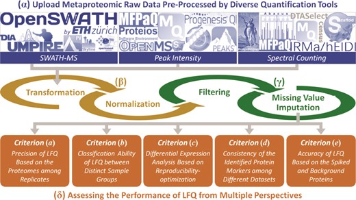
The standard workflow of ANPELA: (α) uploading the raw metaproteomic data preprocessed by 18 quantification tools; (β) data transformation and normalization; (γ) data filtering and imputation; and (δ) the multifaceted performance evaluation from five different perspectives.
As known, a web server is accessible online and can work regardless of users’ operating system and platform, providing advantage over stand-alone applications in terms of accessibility and software update. However, the web server has the disadvantage of being slower than the stand-alone applications due to the time cost of web connection and the shared nature of computational resources [110]. Therefore, the function of ANPELA was realized by not only an online web server but also a local version downloadable directly from ANPELA sites. On one hand, the online web server provided the unique function of evaluating the performance of the whole LFQ workflow from multiple perspectives; on the other hand, the downloaded local tool enabled the discovery of the optimal LFQ(s) by comprehensively ranking all (more than 500) possible LFQ workflows. The official (https://idrblab.org/anpela/) and mirror (http://idrb.zju.edu.cn/anpela/) sites of ANPELA could be readily assessed. Additionally, the source code of the local tool could be downloaded from the home page of these sites and run under R environment without extra installation. The ‘User Manual’ of the local version of ANPELA was also provided in Supplementary Method S4.
ANPELA facilitates the discovery of well-performing LFQ workflows for metaproteomic study
To comprehensively evaluate the level of dependence of LFQ workflows on different metaproteomic data sets, PRIDE database [111] was screened by searching the keywords including ‘Microbiota’, ‘Microbiome’ and ‘Metaproteomic’, which resulted in 106 metaproteomics-related records. Then the corresponding studies of the records were systematically reviewed. By considering several additional criteria [LFQ, the availability of raw intensity data files and the protein database or library to search against, the well-defined parameters (such as isolation scheme and range of retention time) and the clear description on distinct sample groups], eight representative metaproteomic data sets were finally selected for further analysis: PXD006224 [42] (60 metabolic phase & 24 equilibrium phase fecal samples), PXD002882 [112] (21 Crohn’s disease patients & 10 healthy individuals), PXD006129 [113] (14 western style diet & 14 chow-fed mice), PXD006070 [114] (9 corn & 9 grass silage-based samples), PXD003028 [115] (8 people before & 8 people after their breakfast), PXD000987 [116] (8 transverse colon & 8 descending colon samples), PXD005929 [117] (3 surface-exposed & 3 whole cell extracts) and PXD006810 [118] (3 NleB1-infected and 3 wild-type cells). Detailed information of these benchmark data sets could be found in Supplementary Table S3.
Herein, the PCV of protein intensities among replicates for each data set was calculated and applied to assess the ‘precision’ of LFQ. A lower PCV value denoted a more complete reduction of the unwanted signal, which indicated improved LFQ ‘precision’ [20, 98]. The performance of each workflow could be categorized into four groups based on the following PCV values: superior (<0.14) [20, 119], good (0.14~0.3) [119, 120], fair (0.3~0.7) [121] and poor (>0.7) [121]. For 20 representative workflows (as shown in Table 3), their performances on different data sets varied significantly. Taking the first workflow (BOX-MAD-SVD) shown in Table 3 as an example, its performance was superior, good, fair and poor in 1, 2, 4 and 1 data sets, respectively. The variation in LFQ performances among eight metaproteomic data sets are further illustrated in Supplementary Figures S1 and S2. As shown, there was a clear data set-dependent characteristic for the analyzed representative workflows. Thus, for a particular metaproteomic study, it was necessary to assess the performance of each LFQ to discover the well-performing ones, and ANPELA was developed to provide this unique function by assessing each workflow as a whole analysis chain.
Evaluation of different LFQ workflows based on the value of PCV of eight metaproteomic benchmark data sets. The performance of a workflow was categorized into four groups based on the following PCV values: superior (<0.14, double underline), good (0.14~0.3, single underline), fair (0.3~0.7, dotted underline) and poor (>0.7, no underline). The workflow abbreviations are provided in Table 2, and those benchmark data sets are in descending order by their total number of samples (the number of cases versus that of the controls, as listed in the brackets under each data set ID)
| Workflow | PXD006224 (60:24) | PXD002882 (21:10) | PXD006129 (14:14) | PXD006070 (9:9) | PXD003028 (8:8) | PXD000987 (4:4) | PXD005929 (3:3) | PXD006810 (3:3) |
|---|---|---|---|---|---|---|---|---|
| BOX-MAD-SVD | 0.05 | 0.15 | 0.47 | 0.38 | 0.44 | 0.64 | 0.27 | 1.31 |
| BOX-EIG-KNN | 0.26 | 0.48 | 0.32 | 0.19 | 0.26 | 0.22 | 0.10 | 0.28 |
| BOX-QUA-BAK | 0.43 | 0.76 | 0.65 | 0.54 | 0.54 | 0.46 | 0.22 | 0.64 |
| BOX-VSN-CEN | 0.09 | 0.02 | 0.14 | 0.09 | 0.10 | 0.09 | 0.04 | 0.43 |
| CUB-EIG-KNN | 0.29 | 0.52 | 0.36 | 0.21 | 0.29 | 0.25 | 0.11 | 0.31 |
| CUB-MAD-SVD | 0.05 | 0.15 | 0.47 | 0.38 | 0.44 | 0.64 | 0.27 | 1.31 |
| CUB-RLR-CEN | 0.75 | 0.93 | 0.85 | 0.59 | 0.61 | 0.53 | 0.24 | 0.55 |
| CUB-VSN-BAK | 0.11 | 0.18 | 0.15 | 0.76 | 0.12 | 0.11 | 0.05 | 0.60 |
| LOG-EIG-CEN | 0.10 | 0.24 | 0.13 | 0.12 | 0.12 | 0.09 | 0.03 | 0.12 |
| LOG-PQN-ZER | 0.90 | 0.95 | 1.27 | 1.07 | 0.87 | 0.68 | 0.29 | 1.34 |
| LOG-TIC-BAK | 0.21 | 0.31 | 0.23 | 0.45 | 0.21 | 0.17 | 0.09 | 0.72 |
| LOG-VSN-SVD | 0.06 | 0.15 | 0.48 | 0.39 | 0.45 | 0.65 | 0.27 | 1.31 |
| NON-EIG-KNN | 1.08 | 1.55 | 1.07 | 0.69 | 0.96 | 0.82 | 0.32 | 0.82 |
| NON-MAD-SVD | 0.05 | 0.15 | 0.47 | 0.38 | 0.44 | 0.64 | 0.27 | 1.30 |
| NON-VSN-BAK | 0.11 | 0.23 | 0.17 | 0.12 | 0.12 | 0.11 | 0.04 | 0.14 |
| NON-ZSC-CEN | 0.64 | 1.60 | 0.94 | 1.68 | 1.39 | 1.56 | 0.44 | 1.06 |
| POW-CYC-BAK | 1.25 | 2.95 | 2.46 | 1.20 | 4.55 | 10.83 | 1.00 | 6.08 |
| POW-LOW-BAK | 2.26 | 0.41 | 4.71 | 4.26 | 4.08 | 4.41 | 15.87 | 6.64 |
| POW-TMM-ZER | 1.68 | 1.07 | 1.11 | 1.47 | 4.07 | 2.65 | 11.16 | 1.07 |
| POW-VSN-CEN | 0.19 | 0.26 | 0.28 | 0.25 | 0.32 | 0.43 | 0.14 | 0.33 |
Besides metaproteomics, it was of great interest to evaluate the LFQ workflow on further proteomics data sets. As newly emerging technique [122], the ‘sequential windowed acquisition of all theoretical fragment ion mass spectra’ (SWATH-MS) was reported to provide much more comprehensive detection and accurate quantitation of proteins compared to traditional acquisition techniques [122]. Therefore, seven SWATH-MS proteomic data sets were collected from the PRIDE database [111] following the similar process of metaproteomic data sets collection. These benchmark data sets included PXD001064 [123] (72 monozygotic & 44 dizygotic twins blood samples), PXD003972 [124] (20 wild-type & 20 GRB2 knock-in mice), PXD004880 [125] (18 ‘Down syndrome’ patients & 18 healthy individuals plasma samples), PXD000672 [126] (18 tumorous & 18 non-tumorous kidney tissue biopsies), PXD006106 [127] (10 formaldehyde-treated & 10 -untreated HeLa), PXD003278 [128] (6 siRNA-treated & 6 PRPF8-depleted Cal51 cell samples) and PXD002952 [20] (3 yeast 30% versus Escherichia coli 5% & 3 yeast 15% versus E. coli 20% mixtures). Detailed information of these 7 data sets could be found in Supplementary Table S3, and the performances of the same set of 20 representative LFQ workflows in Table 3 on these 7 SWATH-MS proteomic data sets were provided in Supplementary Table S4. Similar to the findings of metaproteomic data sets, the performances of a given LFQ on seven different sets of SWATH-MS data varied greatly. Taking the first workflow (BOX-MAD-SVD) as an example, it performed ‘superior’, ‘good’, ‘fair’ and ‘poor’ in 5, 0, 1 and 1 data sets, respectively (Supplementary Table S4), which showed similar data set-dependent characteristic as for those metaproteomic data sets.
As shown in Table 3 and Supplementary Table S4, some workflows were found to provide mainly ‘superior’, ‘good’, ‘fair’ or ‘poor’ PCV performance. These findings inspired us to further investigate whether there was any general guideline on the selection of consistently well- or poorly performed workflows across various data sets. To achieve this, those eight metaproteomic and seven SWATH-MS proteomic data sets were further analyzed to assess the ‘robustness’ of LFQ performance. First, the ‘robustness’ of LFQ performance between any 2 of 15 studied data sets (defined by the amounts of overlapped workflows with the same level of performances between two data sets) was calculated. Since the number of 2 combinations from those 15 studied data sets (|${C}_{15}^2$|) equaled to 105, 4 error bars (in dark gray) were drawn in Supplementary Figure S3A to indicate the amounts of the overlapped workflows of consistently ‘superior’, ‘good’, ‘fair’ or ‘poor’ performance between any 2 of those 15 studied data sets. Then the ‘robustness’ of LFQ performance among 8 metaproteomic and among all 15 studied data sets was calculated, and the amounts of the overlapped workflows performing consistently ‘superior’, ‘good’, ‘fair’ or ‘poor’ were shown in Supplementary Figure S3A (blue bars for the metaproteomic data sets and orange bars for all 15 studied data sets). Obviously, with the accumulation of the analyzed data sets (from 2 to 8 to 15 in Supplementary Figure S3A), the amounts of overlapped LFQs decreased substantially (from ~161 to 53 to 33 and from ~242 to 129 to 97 for ‘superior’ and ‘poor’, respectively), and there was no overlapped workflow consistently performing ‘good’ and ‘fair’ across 8 and 15 data sets. These indicated a dramatic reduction of the ‘robustness’ of LFQ performance with the accumulation of the analyzed data sets.
As shown in Supplementary Figure S3A, there were 33 and 97 workflows performing consistently ‘superior’ and ‘poor’ across all 15 studied data sets. To investigate the probabilities of each processing method appearing in the consistently ‘superior’ performing workflows, Supplementary Figure S3B was drawn. The occurrence probabilities of some processing methods were found to be higher than the others. Moreover, Supplementary Figure S3C was provided to show the frequency of each method in consistently ‘poor’ performing workflows, and some methods were found to appear more frequently than others. However, considering the dramatically reduced amounts of overlapped workflows (from ~161 to 33 for ‘superior’, from ~242 to 97 for ‘poor’) with the accumulation of the analyzed data sets (Supplementary Figure S3A), it should be very difficult to summarize a general guideline for selecting the consistently well- or poorly performing workflows, especially when more data sets are included for further analysis. Thus, for a specific data set, an independent performance assessment on various LFQ workflows is required, and tools like ANPELA are recommended.
Feasibility of discovering the LFQ performing consistently well under two distinct criteria
Five well-established criteria [20, 59–62] (each with distinct underlying theory) are now available to evaluate the performance of LFQ workflows. Herein, the benchmark data set PXD006224 [42] was collected to analyze and compare the assessment results based on different criteria. As demonstrated in Figure 2A and B, two distinct criteria, (a) precision and (d) reproducibility, were utilized to assess and rank the performance of 560 LFQ workflows. In particular, Figure 2A ranked the LFQ workflows based on their ‘precision’ (measured by PCV value). The cut-off (≤0.7) for a ‘desired’ PCV [121] resulted in 144 workflows with good performance (light orange). Figure 2B ordered the LFQ workflows by their ‘reproducibility’ (measured by ‘CS’). Both figures demonstrated significant variations among the performances of different LFQ workflows (from |${e}^{-6.9}$| to |${e}^{3.7}$| for PCVs; from 38.6 to 106.5 for ‘CSs’). Due to these variations, the performance of each LFQ workflow should be assessed before any metaproteomic study, and ANPELA could be a handy tool for providing such important information.
![Performance assessment of LFQ workflows with the benchmark microbiome data set (PXD006224 [42]) from multiple perspectives. (A) precisions of different LFQ workflows were assessed by PCVs. Cut-off (≤0.7) for ‘desired’ PCVs [121] resulted in 144 workflows of good performance (in light orange background). (B) reproducibility of various workflows was evaluated by the CSs. (C) performance of workflows was collectively assessed by both PCVs and ‘CSs’. The dots indicate the rank of each LFQ workflow, as evaluated by PCVs and ‘CSs’, with the possible workflow used in Tilocca’s pioneering study [42] shown as green dots. The dots accumulated within the purple dash line square were considered as the well-performing workflows under both criteria (a) precision and (d) reproducibility. (D) the top 50 overall ranked workflows by both criteria together with their ranks by each independent criterion.](https://oup.silverchair-cdn.com/oup/backfile/Content_public/Journal/bib/21/2/10.1093_bib_bby127/4/m_bby127f2.jpeg?Expires=1749114434&Signature=gGgAIgKh7AfeZO-4aNPkVBiq6DIBnzAgJSZlq~GZv~RLMe1e2uJOH5z38o507BT62gutv1Z494bEDj3RDYC9aFxEIl0urC1re7deQdcosoUthZ41FUCq3HKC~nE4UBQCLJqT6hsjv1nzCaAImS686SlrDDTh9MvFRiqjbEVep4BI0aUXF6yFVL3ijqSDtXoG-zNapHtGDKteukcSuxAPlpTBmw-1WJhUntQ17VizH9BTEvPps9xKm3Ox~n1UMuMMFlA1~xXertorFV1lOr3-huopHz5TxyTaSk4uE4ss7qo1cMxI8CwfYUaR4k2QqlvkXNs1fbTM8EmubiY~Y~C2IA__&Key-Pair-Id=APKAIE5G5CRDK6RD3PGA)
Performance assessment of LFQ workflows with the benchmark microbiome data set (PXD006224 [42]) from multiple perspectives. (A) precisions of different LFQ workflows were assessed by PCVs. Cut-off (≤0.7) for ‘desired’ PCVs [121] resulted in 144 workflows of good performance (in light orange background). (B) reproducibility of various workflows was evaluated by the CSs. (C) performance of workflows was collectively assessed by both PCVs and ‘CSs’. The dots indicate the rank of each LFQ workflow, as evaluated by PCVs and ‘CSs’, with the possible workflow used in Tilocca’s pioneering study [42] shown as green dots. The dots accumulated within the purple dash line square were considered as the well-performing workflows under both criteria (a) precision and (d) reproducibility. (D) the top 50 overall ranked workflows by both criteria together with their ranks by each independent criterion.
Moreover, the performance of LFQ collectively assessed by both criteria, (a) precision and (d) reproducibility, was shown in Figure 2C. As illustrated, among those 144 highest-ranked workflows by PCV value, only 44 (30.6%, accumulated within the purple dash line square of Figure 2C) were found to perform well under the criterion (d) reproducibility. Considering the large number of possible workflows (560 in total, shown as dots in Figure 2C), only a small fraction (~7.9%) could be considered as the well-performing ones by both criteria. Furthermore, the workflow used in Tilocca’s pioneering study [42] was identified and mapped in Figure 2C (green dots). Since Tilocca’s study mentioned only the transformation method applied, all workflows (96 in total) containing that method were highlighted as green dot. Eight (8.3%) out of these 96 were considered as well performing by both criteria (within purple dash line square). Supplementary Table S5 provided a full list of LFQ workflows ranked independently by the ‘precision’ or ‘reproducibility’. As shown, the ranking results of two criteria were inconsistent with each other. Due to the independent nature of these two criteria [47], the collective consideration of both criteria was proposed here to give an overall ranking to each workflow. Particularly, the overall ranking was defined by the sum of the ranks for two criteria (the smaller the sum is, the higher the LFQ workflow ranks). Taking the LFQ workflow (LOG-EIG-KNN) in Supplementary Table S5 as an example, its independent ranks by both criteria were not so high (ranked 47th and 19th by criterion (a) and (d), respectively), but it was the one of the best overall ranking due to its well-balanced performances between two criteria. Figure 2D gave the top 50 overall ranked workflows together with their ranks by independent criteria (the workflows highlighted in green indicated those LFQs used in Tilocca’s study [42]).
Similar to the above analysis, the same strategy was applied to another SWATH-MS-based benchmark data set PXD001064 [123]. The performance ranks by two distinct criteria, (a) precision and (d) reproducibility, were illustrated in Supplementary Figure S4A and B, and the performances of LFQs collectively evaluated by both criteria were shown in Supplementary Figure S4C. Similar to metaproteomic data set PXD006224 analyzed above, among the 280 highest-ranked workflows by one criterion (PCV values), only 14 (5.0%, accumulated in the purple dash line square of Supplementary Figure S4C) were found to be highly ranked by another (‘CSs’). That is to say, among all 560 workflows (the dots in Supplementary Figure S4C), only very small fraction (~2.5%) could be considered as the well-performing ones by both criteria. The original workflows (five in total) used in Liu’s study [123] for analyzing PXD001064 data set were highlighted as green dots in Supplementary Figure S4C. As shown, three out of these five were suggested by criterion (a) to be the ‘desired’ workflows, but none of the five workflows was found to be well performing under both criteria (no green dot in purple dash line square). Supplementary Figure S4D gave the top 50 overall ranked workflows together with their ranks by each independent criterion. In summary, based on the analysis on two benchmark data sets (one metaproteomic and another SWATH-MS proteomic data sets), the selection of the most suitable criterion for a specific biological problem should be determined by the innate nature of the given data set. As these criteria complement one another [20, 52, 59–62], it is essential to collectively employ them for assessing the performance of LFQ workflow, which further made ANPELA distinguished from other available tools.
ANPELA enables the performance assessment of LFQ workflows from multiple perspectives
The assessment and subsequent performance ranking from multiple perspectives in ANPELA was realized by a variety of metrics. These metrics included PCV value for criterion (a) precision [20], classification accuracy for criterion (b) classification ability [95], level of uniformity of P-value distribution for criterion (c) differential expression analysis [101], CS value for criterion (d) reproducibility [107] and degree of correlation between the measured and expected logFCs of protein intensity for criterion (e) accuracy [50]. Based on these metrics, the performances of 560 LFQ workflows could be ranked separately, and five ranking numbers were assigned to each workflow by the five corresponding criteria. Due to the independent nature of the five criteria [47], the collective consideration of multiple criteria was proposed in this study and realized in ANPELA for providing the overall ranking to all 560 workflows. Particularly, the overall ranking of a given workflow was defined by the sum of multiple ranking numbers under multiple criteria (the smaller the sum is, the higher the LFQ workflow ranks). Taking the metaproteomic benchmark data set PXD006129 (including 14 western style diet & 14 chow-fed mice) [113] as an example, the overall ranking of the performances of 560 workflows on this particular data set was calculated and the top 100 ranked LFQs were provided in Figure 3A. Since there is no spiked protein in this data set, only four criteria (a), (b), (c) and (d) were collectively assessed. As shown, the performance ranking under each criterion was represented by colored rectangles (the top-ranked LFQ was colored by exact blue. With the increase of ranking number, the color changed gradually toward orange with the last-ranked LFQ shown in exact orange). Based on the comprehensive ranking shown in Figure 3A, the selection range of LFQ workflows could be significantly narrowed down, and it is thus possible for the readers to discover the optimal workflows for their own data set.
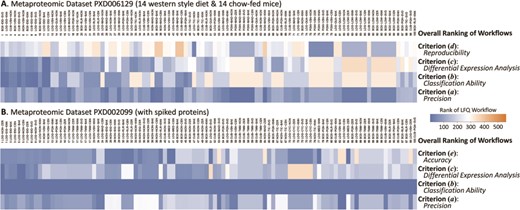
Overall ranking of the performances of LFQ workflows on the metaproteomic data sets (A) PXD006129 with 14 western style diet and 14 chow-fed mice and (B) PXD002099 containing 48 UPS1 proteins spiked with five different concentrations. Since there is no spiked protein in data set PXD006129, only four criteria (a), (b), (c) and (d) were collectively assessed. Since the sample sizes of both case and control in PXD002099 were very small (3 versus 3), it was inappropriate to assess the quantification performance base on criterion (d) reproducibility, and only four criteria (a), (b), (c) and (e) were considered. The performance ranking under each criterion was represented by colored rectangles (the top-ranked LFQ was colored by exact blue). With the increase of ranking number, the color changed gradually toward orange with the last-ranked LFQ shown in exact orange.
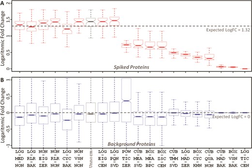
The accuracy of 20 representative LFQ workflows based on (A) spiked and (B) background proteins for two distinct data sets of different protein concentration (10 versus 25 fmol/μL) in PXD002099. The workflows were ordered by the level of deviations between the median and expected logFCs of spiked proteins. Expected logFCs for the background and spiked proteins were 0 and 1.32, respectively. The workflow abbreviation was provided in Table 2. ‘Unnorm.’ denotes unnormalized data.
Because of the tremendous computational workload required for assessing 560 workflows, it is too time- and resource-consuming to make the comprehensive assessment service online. Therefore, an alternative way of enabling the evaluation on user’s local computer was provided as a stand-alone ANPELA. This version could be downloaded from both official (https://idrblab.org/anpela/) and mirror (http://idrb.zju.edu.cn/anpela/) sites and provided the same sets of assessment metrics and plots as that of the online ANPELA. Moreover, this local version tool could further provide an overall performance ranking for all 560 workflows in the format of not only a figure (shown in Figure 3) but also a ‘CSV’ table (including detail results of assessing metrics, ranks by independent criteria and overall ranking). The exemplar input/output files could be simultaneously downloaded together with the source code of the stand-alone tool from ANPELA websites. The installation of R environment was required before running ANPELA and was provided in ‘User Manual’ (downloadable from websites) and Supplementary Method S4. Both ‘User Manual’ and exemplar files could help users to get familiar with this tool as soon as possible.
ANPELA validates the accuracy of LFQ workflows based on spiked and background proteins
Spiked protein is frequently adopted to evaluate the performance of an LFQ workflow [52, 129]. A workflow with desirable accuracy should not only maintain unbiased variation in background proteins between sample groups (the expected logFC between the case and control equals to zero) but also make the variation in spiked proteins biased by viewing the expected abundance ratios as golden standard [50, 101]. Herein, the ability of ANPELA to validate the accuracy of LFQ workflows based on spiked proteins was analyzed using benchmark data PXD002099 with known ‘ground truth’ of variant proteins (48 UPS1 proteins spiked into yeast proteome digest with five different concentrations 2, 4, 10, 25 and 50 fmol/μL) [61]. A random combination of any 2 of these different concentrations could therefore result in 10 pairs of sample group with distinct concentration. Taking the pair of 10 versus 25 fmol/μL as an example, the accuracy of the 20 representative LFQ workflows were determined by considering the spiked (Figure 4A) and background (Figure 4B) proteins. All workflows were found to be able to maintain the unbiased variations of background proteins between sample groups, but only some workflows could make the variation in spiked proteins biased according to the expected abundance ratio (|${\mathrm{logFC}}_{expected}=1.32$| in this case). With reference to the logFC of unnormalized data (the gray boxplot in Figure 4A), several workflows demonstrated good performance in guaranteeing biased variation in spiked proteins. The variance stabilization normalization (VSN) described in Valikangas’s study [50] as ‘performed well in differential expression analysis’ was identified well performing (the 6th ranked as shown in Figure 4) in this study. The well-performing workflows (in Figure 4) also included LOG-MED-NON, LOG-RLR-BAK, NON-EIG-ZER, NON-RLR-NON and LOG-CYC-BAK. For the remaining nine pairs of sample group, the accuracy of the same set of 20 representative workflows were analyzed and illustrated in Supplementary Figures S5–S13. As shown, the accuracy of different representative workflows for a specific concentration varied greatly, and the accuracy ranks of a particular workflow for different pairs also changed substantially. Table 4 gave an overview of the LFQ workflows performing better than unnormalization (indicated by circle). No LFQ workflow was found performing consistently better across all pairs of sample group, and the number of these well-performing workflows for different data set pairs varied from 1 to 15.
Overview of the performance of 20 representative LFQ workflows assessed by criterion (e) accuracy. The LFQ workflows performing better and worse than unnormalization were represented by circle and cross, respectively
| Workflow | 2 versus 4 | 2 versus 10 | 2 versus 25 | 2 versus 50 | 4 versus 10 | 4 versus 25 | 4 versus 50 | 10 versus 25 | 10 versus 50 | 25 versus 50 |
|---|---|---|---|---|---|---|---|---|---|---|
| NON-VSN-NON | × | Ο | Ο | Ο | Ο | Ο | Ο | Ο | Ο | Ο |
| LOG-CYC-BAK | × | Ο | Ο | Ο | Ο | Ο | Ο | Ο | × | Ο |
| LOG-MED-NON | × | Ο | Ο | Ο | Ο | Ο | Ο | Ο | × | Ο |
| LOG-PQN-SVD | × | Ο | Ο | Ο | Ο | Ο | Ο | × | Ο | Ο |
| LOG-RLR-BAK | × | Ο | Ο | Ο | Ο | Ο | Ο | Ο | × | × |
| NON-RLR-NON | × | Ο | Ο | Ο | Ο | Ο | Ο | Ο | × | × |
| NON-EIG-ZER | × | × | Ο | Ο | Ο | × | × | Ο | × | Ο |
| BOX-MEA-BPC | × | Ο | × | × | Ο | × | × | × | × | × |
| BOX-VSN-BAK | × | Ο | × | × | Ο | × | × | × | × | × |
| BOX-ZSC-CEN | × | Ο | × | × | Ο | × | × | × | × | × |
| CUB-MEA-SVD | × | Ο | × | × | Ο | × | × | × | × | × |
| LOG-EIG-CEN | Ο | × | × | × | × | × | × | × | Ο | |
| BOX-CYC-KNN | × | × | × | × | Ο | × | × | × | × | × |
| CUB-QUA-NON | × | × | × | × | Ο | × | × | × | × | × |
| CUB-TMM-SVD | × | × | × | × | Ο | × | × | × | × | × |
| LOG-MAD-ZER | × | × | × | × | Ο | × | × | × | × | × |
| CUB-MAD-BAK | × | × | × | × | × | × | × | × | × | × |
| LOG-TIC-CEN | × | × | × | × | × | × | × | × | × | × |
| POW-TIC-ZER | × | × | × | × | × | × | × | × | × | × |
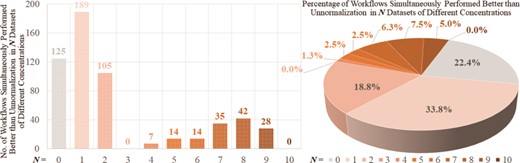
Numbers and percentages of the LFQs performing better than unnormalization among all workflows assessed by criterion (e) accuracy.
Supplementary Table S6 provided the degree of correlation (between the measured and expected logFCs of protein intensity) of LFQ workflow for the data sets of different concentrations (2 versus 4 fmol/μL, 2 versus 10 fmol/μL, 2 versus 25 fmol/μL, 2 versus 50 fmol/μL, 4 versus 10 fmol/μL, 4 versus 25 fmol/μL, 4 versus 50 fmol/μL, 10 versus 25 fmol/μL, 10 versus 50 fmol/μL and 25 versus 50 fmol/μL). The number in each cell of Supplementary Table S6 indicated the median deviation of spiked proteins ± standard deviation. The number highlighted in green and bold was the workflow of better accuracy than unnormalization. As shown, no LFQ workflow was discovered to perform consistently better than unnormalization across all 10 pairs of sample group, and the majority of the workflows performed well only in very limited pairs (~75% of the 560 were well performing in no more than 2 pairs; Figure 5). The inconsistency of the performances among different pairs indicated the data set-dependent nature of LFQ workflow, and a case-by-case performance assessment for a given data set is thus required. In sum, ANPELA demonstrated good capacity for validating the accuracy of an LFQ workflow by preserving the true biological variation of spiked proteins, which could be used to discover the optimal workflow for a metaproteomic study with the gold standard of the expected protein abundance ratio.
Besides ‘accuracy’, other four criteria could be collectively considered in ANPELA. A metaproteomic benchmark data set PXD002099 (48 UPS1 proteins spiked into the yeast proteome with five different concentrations) [61] was therefore collected as example. The overall ranking of the performances of 560 workflows on this data set was calculated and the top 100 ranked LFQs were provided in Figure 3B. Since the sample sizes of the cases and controls were small (3 versus 3), it was inappropriate to assess the quantification performance using criterion (d) reproducibility, and only criteria (a), (b), (c) and (e) were considered. Based on the ranking in Figure 3B, the selection range of LFQs was greatly narrowed down by collectively considering those independent criteria.
Conclusions
ANPELA allows the users to directly analyze the standard output files of popular quantification tools, and its multifaceted strategies for performance assessments could collectively improve the reproducibility, precision and accuracy of LFQ in metaproteomic studies. ANPELA has a unique ability to evaluate the performance of the whole workflow and enables the identification of the optimal LFQ(s) by the comprehensive performance ranking of all 560 workflows. Thus, it has great potential for applications in metaproteomic and other studies requiring LFQ techniques, as many features are shared among proteomic studies. To enhance the accessibility of ANPELA, a mirror site (http://idrb.zju.edu.cn/anpela/) was constructed as the backup of the official ANPELA site (https://idrblab.org/anpela/).
Author Contributions
F.Z. conceived the idea and supervised the work. J.T., J.F. and Y.W. performed the research. J.T., B.L., Y.L. and J.F. constructed the web server, developed the software and wrote the scripts. J.T., J.F., Y.W., Y.L., Q.Y., X.C., J.H., X.L., Y.C. and W.X. prepared and analyzed the data. F.Z. wrote the manuscript.
An online tool ANPELA is presented to enable performance assessment of the whole LFQ workflow (collective assessment by five well-established criteria with distinct underlying theories).
ANPELA enables the identification of the optimal LFQ(s) based on the comprehensive performance ranking of all 560 workflows.
ANPELA not only automatically detects the diverse formats of data generated by all quantification tools but also provides the most complete set of processing methods among the available web servers and stand-alone tools.
Systematic validation using metaproteomic benchmarks revealed ANPELA’s capabilities. It is publicly accessible at https://idrblab.org/anpela/.
Funding
National Natural Science Foundation of China (81872798); National Key Research and Development Program of China (2018YFC0910500); Innovation Project on Industrial Generic Key Technologies of Chongqing (cstc2015zdcy-ztzx120003); Fundamental Research Funds for the Central Universities (2018QNA7023, 10611CDJXZ238826, 2018CDQYSG0007, CDJZR14468801, CDJKXB14011).
Jing Tang, Jianbo Fu, Yunxia Wang, Bo Li, Yinghong Li, Qingxia Yang, Xuejiao Cui, Jiajun Hong, Xiaofeng Li are students of the College of Pharmaceutical Sciences in Zhejiang University, China and jointly cultivated by the School of Pharmaceutical Sciences in Chongqing University, China. They are interested in the area of bioinformatics and proteomics-based target identification.
Feng Zhu is a professor of the College of Pharmaceutical Sciences in Zhejiang University, China. He got his PhD degree from the National University of Singapore, Singapore. His research group (https://idrblab.org/) has been working in the fields of bioinformatics, OMIC-based drug discovery, system biology and medicinal chemistry. Welcome to visit his personal website (https://idrblab.org/Peoples.php) at any time.
