


Abstract
The use of signalling pathway hypergraphs represented as process description diagrams is steadily becoming more pervasive in the field of biology. This makes ever more evident the necessity for an effective automated layout that can replicate high-quality manually drawn diagrams. The complexity and idiosyncrasies of these diagrams, as well as the specific tasks the end users perform with them, mean that a layout must meet many requirements beyond the simple metrics used in existing automated computational approaches. In this paper we outline these requirements, examine existing ones and describe new ones. We demonstrate state-of-the-art layout techniques enhanced with novel functionalities to meet part of the requirements. For comparatively small signalling pathways our enhanced algorithm provides results close to manually drawn layouts. In addition, we suggest technical approaches that may be suited for fulfilling the identified requirements currently not covered.
Introduction
An increasingly large number of pathways appear as diagrams in process description formats (state transition diagrams, process diagrams) such as the Systems Biology Graphical Notation (SBGN) [1] Process Description and the graphical notation used in CellDesigner (www.celldesigner.org). Visual representations of such diagrams are widely used, for example, in Reactome [2] and PANTHER [3] pathway databases, in the Atlas of Cancer Signalling Networks [4], the Parkinson’s disease map [5]; they also appear in many visualisations of models in the BioModels Database [6] and in many of the over 200 other resources in the list of available pathway databases at Pathguide [7]. The design of pathway diagrams is done with varying degrees of aesthetic appeal and readability. The resources that store pathway information in Systems Biology Markup Language (SBML) [8] and Biological Pathway Exchange (BioPAX) [9] formats often do not include layout information while visualisation of models is needed and there are tools that provide the corresponding layout functionalities for SBML, for example CySBML [10], Arcadia [11] (http://sbml.org/SBML_Software_Guide) and for BioPAX, for example ChiBE [12] and BioLayout Express3D [13].
Process description diagrams are a form of hypergraph, that is, a graph where edges may connect more than two nodes [14]. In these hypergraphs, nodes correspond to biological entities (macromolecular, complexes, metabolites, etc.) and hyper-edges correspond to process glyphs with the connected edges. For example, the process of a heterodimer formation involves three nodes including two macromolecules consumed in such a process and the produced heterodimer.
Within the fields of graph drawing and network visualization, automatic graph layout is a highly studied topic. The aforementioned list of data resources and applications demonstrates that there is a clear demand for layout algorithms that would allow more efficient manipulation of pathway information and advanced visualisation.
The use of automatic layout algorithms in systems biology is limited as the available algorithms fall short of expectations for the figures generated to be used in publications and for expressing the intended message. The motivation of this work is the necessity to make automatic layout possible for signalling pathways on demand, while keeping them easily readable and useful as conceptual views and as an expression of ‘stories’ that biologists try to convey when they build these diagrams. To achieve this, we need to define the criteria and principles that constitute a well-designed pathway diagram and to transform those principles into an algorithm that would produce layouts able to compete with, or even outperform, human-drawn layouts.
The two most relevant works related to this topic are those of Kieffer et al. [15] and Genc and Dogrusoz [16]. The first contains a comprehensive evaluation of requirements aimed at producing human-like layout results for metabolic diagrams. The second work tailors a force-directed layout approach to support some important requirements specific to SBGN Process Description maps.
The goal we set out is to build an aesthetically satisfying layout algorithm for signalling pathways in the format of Process Description diagrams. By ‘aesthetically satisfying’ here we mean that it would be hard to distinguish diagrams developed manually from diagrams automatically laid out and that these diagrams are aesthetically appealing to the viewers.
The immediate objectives of this work are (1) to identify and list the requirements; (2) to demonstrate the effectiveness of our approach by showing the output of an implementation of a set of the requirements using comparatively small examples; (3) to outline a set of future research directions to improve the approach further.
In this paper, we specifically focus on signalling hypergraphs (i.e. process description diagrams that describe cellular signalling); however, we expect that the discussed approaches can be applied to metabolic and gene regulatory diagrams with minor additional adjustments.
This paper is organised as follows: first, we outline general requirements gathered from the literature and the SBGN specification [17] as well as the specific requirements we define. Then, we present relevant state-of-the-art techniques that build the basis for our layout approach along with enhancements to start addressing the identified requirements. Afterwards, we show and discuss layouts produced by our algorithm and, finally, conclude with suggestions for future approaches.
Requirements
This section seeks to outline the complete set of requirements identified from different sources related to drawing signalling hypergraphs for describing biological processes with the focus on producing a valid and efficient layout. The requirements are divided into three parts which consist of R1, established graph drawing requirements, R2, existing pathway hypergraph specific requirements for process description diagrams and finally, R3, novel and underexplored pathway specific requirements (Table 1).
The identified requirements for the layout of signalling pathway hypergraphs
| Group | Requirement |
| R1. Established requirements described in the literature | a. Edge crossings |
| b. Uniform edge lengths | |
| c. Minimising edge bends | |
| d. Maximising edge crossing angle | |
| e. Symmetry | |
| f. Unit grid alignment | |
| g. Horizontal and vertical edge routing | |
| h. Emphasizing clusters | |
| i. Sub-trees placed outside | |
| j. Low-stress conformations | |
| R2. Specific requirements for signalling hypergraphs | a. Node, edge and label drawing |
| b. Process drawing and ports | |
| c. Submap drawing and terminals | |
| d. Containers and nested layout | |
| e. Cloning | |
| f. Miscellaneous suggested requirements | |
| R3. Novel and underexplored requirements | a. Maintain a global mental map across different layouts |
| b. Layout elements of cycles on a convex scaffold | |
| c. Sacrifice aesthetics for readability |
Established requirements described in the literature
Aesthetics define requirements for general properties of graph drawings that should be minimized/maximized to increase readability. Some of the most common aesthetic criteria are minimizing the number of edge crossings, edge bends, required area, overlapping elements as well as maximizing symmetry and uniform edge length, which are covered by the requirements R1a-e. More comprehensive overviews of aesthetic criteria are given in [18, 19].
It is challenging to optimize a given set of aesthetics rules since they often conflict with each other, e.g. minimizing the number of crossings versus maximizing symmetry. Furthermore, the precedence of aesthetics often depends on the specific application domain and individual user preferences.
Purchase and co-authors [20, 21] analysed the impact of different aesthetics on the readability of graph drawings. It was determined that the most important criterion was minimizing edge crossings followed by minimizing bends and maximizing symmetry. Edge crossing cannot always be eliminated and further work found that maximising the crossing angle reduced task completion time for simple tasks [22].
More recently, Purchase and co-authors investigated which graph drawing aesthetics people favour when they create their own drawings [23]. Compared with most of the previous studies on graph drawing aesthetics, which mainly considered the interpretation of existing drawings, the participants had to draw the graphs from scratch and produce a ‘nice’ layout. Again, minimizing edge crossings was found out to be the most important criterion. Users also preferred placing nodes on an underlying (virtual) unit grid as well as horizontal or vertical edge segments (requirements R1f, g). In addition, users emphasized clusters of nodes and preferred edges of equal length (requirement R1h).
In another recent work [15], the participants manually improved the given layout of small graphs and, in a second step, chose the best layout obtained from the first step. The authors identified two novel user preferences: the creation of ‘aesthetic bend points’ to emphasize symmetry as well as the placement of subtree components in the outer face of the graph (requirement R1i). Besides these two findings, they also found correlations indicating that users prefer compact drawings, grid-like node placement, symmetry, a small number of edge crossings and bends, as well as a low deviation of edge length and a low stress (requirement R1j). These evaluations of various aesthetics have established a fundamental set of requirements for graph layout.
The preceding aesthetics were defined and evaluated in the context of two-dimensional graph layout. One possible approach to reduce edge intersections and allow more space to organise and structure a network is to use three dimensions rather than the usual two [24]. User evaluations of three-dimensional layout have shown it to be of benefit when viewed using stereoscopy (or another depth cue such as motion) and on graphs with limited or random structure [25, 26]. More recently, immersive approaches such as using Head Mounted Displays or a CAVE environment were shown to be beneficial [27] and were used for biological data visualisation [28]. However, the SBGN process description specification for biological pathway visualisation is defined only for two-dimensional layouts and in this work we limit our consideration of requirements and layout approaches to those that are relevant to two-dimensional layout.
Specific requirements for signalling hypergraphs
This section details known requirements and guidelines connected with layout and drawing of pathway hypergraphs. They represent to a large extent a summary of the SBGN specification [17] of requirements important for a valid drawing of SBGN elements and diagrams. Figure 1 shows an example of such a biological pathway hypergraph drawn in SBGN process description notation. It demonstrates the use of the different elements of the notation discussed in this section, and the reader is invited to refer to this figure when reading the requirements (R2a–R2f) below.
![An example biological pathway with the corresponding system of symbols. A. The IGFR signalling pathway drawn in SBGN Process Description according to the specification [17]. B. The legend represents a reduced set of the glyphs and notations defined in SBGN but covers those relevant for graph layout. A reference card with a complete set of SBGN Process Description glyphs is available at http://sbgn.org/templates. Please note that the SBGN specification does not impose colours, sizes or fonts and though the remaining figures in this work have a different style, they are still valid SBGN graphs.](https://oup.silverchair-cdn.com/oup/backfile/Content_public/Journal/bib/21/1/10.1093_bib_bby099/4/m_bby099f1.jpeg?Expires=1749295475&Signature=lKDKzVQjaipNRrNh5l5~rSem7tQcYicegf8X0SgaDi2PohZ3dU7QQLKKHM6-P-Yqld6q0WgZREJhV5aKBmkiMoU5K0-tl6O8oy51mbmkQTA1H6BZshL6IJvEc7oo7ol4QdtBWqmbJJtGORlIw7dqatnoYoDC85ZHU5gplw71Dg0lfrMrm0VHKidy~LSD58txL46RaFLDqXUZPUrK5zvahk-XDfnnHN1DBM~kuU8~MV4db~EurzsSsDMFmu70JgemX4RQeB4tqdsVL~bj2unCDoHvxeCellUrSfIlXGFyKzvba8zjuK1Nq7p4IE5S7IQxYTxpBOVdaJC4D2utTT23kw__&Key-Pair-Id=APKAIE5G5CRDK6RD3PGA)
An example biological pathway with the corresponding system of symbols. A. The IGFR signalling pathway drawn in SBGN Process Description according to the specification [17]. B. The legend represents a reduced set of the glyphs and notations defined in SBGN but covers those relevant for graph layout. A reference card with a complete set of SBGN Process Description glyphs is available at http://sbgn.org/templates. Please note that the SBGN specification does not impose colours, sizes or fonts and though the remaining figures in this work have a different style, they are still valid SBGN graphs.
Node, edge and label drawing (R2a)
It is strictly forbidden for nodes in the graph to touch or overlap (except for containing nodes), as edges may cross over nodes but crossing their boundary only twice. Additionally, nodes should be oriented horizontally or vertically. Labels should be drawn within the node to which they belong if possible, but may never overlap other labels. Edge labels should not overlap the edge to which they belong. The miscellaneous recommended requirements (R2f) below, list additional suggestions related to edge drawing.
Process drawing and ports (R2b)
The generic process element is depicted as a square box with elements involved in consumption and production linked with two connectors (we can refer to them as ‘ports’) attached to the middle of two opposing sides. The regulatory arcs (stimulation, catalysis, inhibition, modulation, etc.) can be connected to the remaining two sides of the box.
A process node must be drawn in a biological compartment where it has process participants or in the empty space if it spans multiple compartments. If a process and participants all belong to a single compartment, all the connecting edges should be drawn within it.
Process branching points or the process ports, should be placed at a distance comparable to the size of the process symbol.
Submap drawing and terminals (R2c)
The submap is an element that hides its content and displays only terminals on its edge that correspond to an entity it is connected to. These terminals represent connections between an element inside with the same element outside of the submap. Upon request, a tool might expand/collapse the submap within the same map or open it as a different map.
Containers and nested layout (R2d)
Besides the submap element, there are two types of container elements: complexes and compartments. These may contain other elements within them, also in a hierarchical fashion. Complexes are simpler and may not contain compartments or actual processes amongst other constraints, hence, require a simpler layout algorithm as they contain no edges.
Compartment nodes, on the other hand, may contain pathways, and a special feature to consider for their visualisation is the placement of nodes on the compartment boundary. This is typically used for transports, such as proteins taking part in the transport through cell membranes.
Cloning (R2e)
Cloning nodes may be used by an automatic layout routine or by the human curator to avoid long edges connecting to common frequently encountered elements and impacting the readability. The SBGN specification demands that cloned elements be marked as such with a dark bar at the node bottom.
Miscellaneous suggested requirements (R2f)
The elements covered by this requirement section originate from the suggestion section of the SBGN specification and are to some degree similar to general graph aesthetics requirements.
For instance, it is suggested to keep the ratio of width and height in the pathway close to 1:1 and symmetric. Symmetry applies here more to sub-components where parallel and reversible processes are drawn symmetrically. Likewise, if similar sub-components are repeated throughout the map they should be drawn in the same way, so that these sub-structures become evident and easily identifiable by the user.
Here, it is also important to keep related elements close together and arrange them in such a way that the main flow direction is straight vertically or horizontally, preferably starting from top left.
Finally, edge crossings and bends should be avoided, and if edges have to cross, then preferably at a 90° angle.
Novel and underexplored requirements
Some aspects of pathway layout, notably the organisation of its main elements, will be entirely dependent on preferences of the human who curates it. Depending on the ‘story’ that the curator wants to convey to the user, some elements may need central placement and more emphasis than others.
In addition, if the map is updated with a new structure or the layout is regenerated for a subset of the graph, it is important that some elements be placed more or less in the same region. Within the topic of dynamic graph visualisation, the concept of preserving the user’s mental map is used to help users understand a graph as it changes over time. Coleman and Parker [18] suggest, as a dynamic aesthetic for graph layout, that ‘the placement of existing nodes and edges should change as little as possible when a change is made to the graph’. This is often referred to as preserving the mental map. Layout algorithms for dynamic graphs typically consider preservation of the mental map as a constraint as the graph changes over time. Despite this, empirical evidence on the benefit of maintaining a mental map is slight; it may, however, be of benefit for tasks where there is a large number of data elements and the user needs to perform tasks relating to the tracing of long paths, or orientation within a graph, or identifying nodes by name [29]. Biological pathways are traditionally not dynamic graphs; they are, however, large, they contain long paths which must be followed by users to understand processes and they frequently use orientation. Czauderna et al. [30] maintain a mental map when converting pathways from KEGG [31] to SBGN format. In this context, maintaining the mental map is preserving visual features between the layouts when the pathway is converted. Within dynamic graph visualisation, maintaining the mental map means preserving visual features at different points in time, as elements are added and removed from the graph. In the context of pathway layout, we refer to preserving visual features when pathways are filtered, combined or even created from scratch, in relation to a conceptual global mental map of all features related to the biological entities of interest. The goal is to allow a user to quickly reorient and find common elements in the expected places, which is the essence of requirement R3a.
Another requirement relates to the arrangement of flows in the natural reading direction from top to bottom and left to right (R2f). Pathway processes at times represent cycles and are typically positioned in a circular arrangement to emphasise this fact with a clockwise flow. A human-like algorithm should capture these circular structures and arrange their elements accordingly (requirement stated by R3b).
Finally, a human curator will often prefer to sacrifice some established graph layout guidelines in order to satisfy these aesthetics in favour of readability requirements. For instance, compactness of the graph and reduction of edge crossings or edge lengths will have a lower priority, which is here covered by requirement R3c.
Approaches
In this section we describe in detail the techniques we apply for our enhanced approach. We begin with a brief overview of the data preprocessing and tools, then examine the state-of-the-art techniques that we use (Table 2) and finally describe each of the enhanced features with simple illustrative examples.
The approaches applied to the layout of signalling pathway hypergraphs
| Group | Approach |
|---|---|
| A1. Basic state-of-the-art approach | a. TSM framework |
| A2. Enhanced approach implemented in this work | a. Complex nesting: SBGN adjustments for complexes containing nested complexes at times without edges |
| b. Complex packing | |
| c. Flip approach |
| Group | Approach |
|---|---|
| A1. Basic state-of-the-art approach | a. TSM framework |
| A2. Enhanced approach implemented in this work | a. Complex nesting: SBGN adjustments for complexes containing nested complexes at times without edges |
| b. Complex packing | |
| c. Flip approach |
Preprocessing
Biological diagrams represented in SBGN Markup Language (SBGN-ML) format were converted to the yEd GraphML format using the ySBGN tool (https://github.com/sbgn/ySBGN). This allowed us to use the yEd Graph Editor (https://www.yworks.com/products/yed) as an environment for applying layout algorithms.
Basic state-of-the-art approach
The most common approaches for the automatic layout of general graphs are force-directed approaches [32], algebraic approaches [33], layered approaches, as well as the topology-shape-metrics (TSM) approach for orthogonal layouts. Reviews of these different approaches are available [19, 34, 35].
The TSM approach is one of the most popular frameworks for creating orthogonal grid drawings of undirected graphs and there are several refinements and extensions of the basic concept [36–38]. In the following, we review the three phases of the TSM approach and refer to the specific algorithms/heuristics that we choose for our basic implemented approach. Note that our implementation closely follows the description in the dissertation of Markus Eiglsperger [39]:
The planarisation phase calculates a planar embedding of the input graph that is a drawing without edge crossings. Each planar graph has such a drawing. Non-planar graphs are made planar by temporarily replacing crossings with artificial nodes (Figure 2B). A planar embedding divides the plane into regions called ‘faces’. There is always exactly one unbounded region that is called ‘outer face’. Note that a planar embedding can be specified by the cyclic order of the edges around each node. The main objective of this phase is to minimize the number of crossings. Since crossing minimisation of general graphs is non-deterministic polynomial-time hardness (NP-hard), most implementations use heuristic approaches. We use a popular strategy that first calculates a planar subgraph and then routes the remaining edges by means of a shortest-path search in the dual graph [19]. For a planar embedding of an input graph, the dual graph consists of a node for each face. Each edge of the dual graph has a corresponding edge in the input graph that separates the two faces associated with the dual edge’s endpoints (Figure 2C). For the calculation of the planar subgraph, we use the randomised approach [40] that extends the two-phase heuristic technique [41].
The orthogonalisation phase fixes the shape of the edges without changing the planar embedding calculated in the previous phase. Each edge consists of an orthogonal path, i.e. an alternating sequence of horizontal and vertical line segments (Figure 2D). Algorithms that implement this phase try to minimize the number of bends of edges. We use the Kandinsky approach [38] that extends the network flow-based approach of Tamassia [42] and can be applied to general planar graphs with a given planar embedding. We solve the associated optimisation problem with the heuristic technique [39] that usually produces a result with a low bend number.
The compaction phase calculates the final coordinates such that all nodes and bends are placed on a unit grid without producing overlapping elements (Figure 2E). Most approaches try to minimize the required area or edge length at this step. We use a method that first employs a fast linear-time approach to obtain a feasible solution and then improve it by a post-processing step [39]. The calculation of the feasible solution is based on the shape-graph compaction approach [43] and uses a variant of the so-called rectangular decomposition [42], in which each face is made rectangular by introducing additional dummy nodes and edges. The post-processing step is based on a flow-based one-dimensional compaction algorithm [44].
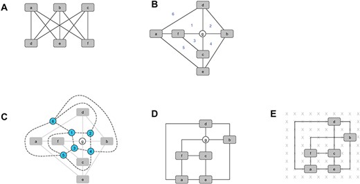
The different phases of the TSM approach. A. The non-planar input graph. B. The result of the planarisation phase where the crossing is replaced by an artificial node ‘g’. The six faces/regions induced by the planar embedding are labelled with numbers where ‘6’ denotes the outer face. C. The dual graph is drawn above the planar embedding. It consists of the blue nodes and the dashed edges. D. After the orthogonalisation phase, each edge is represented by a sequence of horizontal and vertical line segments. E. Final result after applying the compaction phase. All nodes and bends are placed on grid points.
In addition, we have implemented the extensions [45, 46] that allow the application of the above approach to hierarchically clustered graphs where each cluster represents a given subset of nodes that should be placed within a rectangular region. We use clusters to model compartments of pathways.
The enhanced approach implemented in this work
To address the specific needs of process description diagrams, elements such as molecular complexes and compartments need special attention.
Complexes consist of disconnected nodes, i.e. nodes that are visualised without incident edges. Furthermore, they are often built recursively such that a complex may contain other complexes.
Compartments, on the other hand, may consist of small or large pathways, also containing nested compartments. Common to both types of elements is the fact that they contain other graph elements that are isolated from the rest of the graph for complexes or sparsely connected (to the rest of the graph) for compartments. Note that the basic approach already supports hierarchically clustered input graphs and, thus, compartments.
Complex nesting (A2a)
Disconnected cluster structures, such as complexes, cannot be handled by the basic approach. Hence, we process complexes in a recursive fashion from the bottom to the topmost complexes with respect to the clustering hierarchy. After placing the content of a complex, we temporarily replace it with a single node (acting as a placeholder) of appropriate size and then continue with the parent complex, see Figure 3. This strategy has the advantage of reducing the placement of disconnected elements within a complex to a common packing problem. Note that a similar approach was described by Genc and Dogrusoz [16]. Another advantage of this strategy is that the layout of complexes can be handled independently and, thus, we can simply exchange the placement strategy without further modifications of the basic approach.

Illustration of the recursive packing algorithm. A. The input graph. B. Packing of the bottommost complexes. C. Packing of complex ‘a’ where the contained complex ‘b’ is represented as a single node of appropriate size. D. Applying the orthogonal layout algorithm to the graph where the two topmost complexes ‘c’ and ‘a’ are represented as two single nodes. E. The final result in which the artificial nodes are replaced by the packed complexes.
Complex packing (A2b)
Recursive processing allows us to map the layout of the complexes to a common two-dimensional strip packing problem where a set of rectangles (i.e. the elements of a complex) is packed into a strip of fixed width and infinite height such that the height is minimized. We apply the so-called ‘Next-Fit Decreasing Height’ level algorithm [47] that first sorts the rectangles according to their height in descending order and then places them one by one from left-to-right in the current level as long as they fit the given maximum width. If an element does not fit on the current level, the algorithm creates a new level and continues. We apply the algorithm with different values for the maximum width and take the solution that best fits a 1:1 aspect ratio. This approach is fast and produces satisfying results in practice.
Besides applying a packing algorithm, our implementation also supports keeping the content of complexes as it is, assuming that the user already placed the content manually. Of course, for future work, it is also possible to implement more specific strategies that place the elements according to some semantic rules.
Flipping of sub-components (A2c)
In order to produce more human-like layout results, we further use a post-processing step for the planarisation phase that attempts to ‘flip’ subcomponents from one face into another according to specific rules. We consider each subcomponent to be a subgraph that connects to the remaining graph with a single edge. More precisely, we identify such components by first determining the set of articulation points. In graph theory, an articulation point corresponds to a node whose removal disconnects the graph into multiple components [48]. Then, we determine the subset of articulation points that are incident to different faces. In Figure 4A, there are two such points that are drawn as small black rectangles. For each of them, we have to check the components that would arise when we remove the point. If one of these components is connected to the point by a single edge, we can change the face of this component by modifying the cyclic order of the edges around the point. Note that, in general, we can place the component on any face incident to that point without introducing new crossings. Hence, without a specific strategy, the algorithm has no preference on how to choose this face.
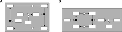
Illustration of the subcomponent flipping. A. Example without flipping. B. The enhanced result that uses our flipping strategy. The algorithm identifies the two articulation points that are incident to different faces (the small black rectangles) and changes the cyclic order of their edges such that the two subcomponents are placed outside the cycle. While, in general, our strategy does not reduce the overall area, it often produces more readable drawings where the cycles and components can be better recognized.
To improve the result of the embedding phase, we apply the following rules to determine a suitable face: if a subcomponent is contained within a user-specified cycle (but does not belong to the cycle), we prefer a face outside of the cycle as shown in the example of Figure 4. Furthermore, if possible, we place subcomponents on the outer face or, if they belong to a compartment, at the border of the group node. While, in general, this strategy does not reduce the required area, it often produces cycles with shorter edges and improves the recognition of both cycles and components. It is especially suited for sparse graphs that usually contain a large number of subcomponents.
Runtime complexity
For a given pathway, let |$n$| denote the number of nodes, |$m$| the number of edges, |$c$| the number of compartments, |$h$| the maximum nesting depths of compartments and |$x$| the number of edge crossings in the resulting drawing. The runtime complexity of the basic state-of-the-art algorithm is dominated by the planarisation with |$O(mx\,+\,{m}^2c\,+\, mnc)$| [45] and the orthogonalisation with |$O({(n\,\cdotp h)}^{7/4}\sqrt{\mathit{\log}\,n})$| [46]. In practice, pathways are usually sparse graphs in such a way that we can safely assume that |$m$|, |$c$| and |$x$| are bounded by |$O(n)$| and |$h$| by a constant value which results in an overall runtime complexity of |$O\!\left({n}^3\right)$| for such graphs. Note that all of our example diagrams (including those in Supplementary Materials) were calculated in less than one second on a standard desktop computer.
Our enhancements described above do not increase the overall runtime complexity. The runtime of the recursive packing of the complex nodes is dominated by the sorting of the elements according to their size which requires |$O\left(n\log n\right)$| [48]. To obtain an aspect ratio close to 1:1, we repeat this step multiple times. However, since we bound the number of iterations by a fixed constant value, the runtime remains |$O\left(n\log n\right)$|. For the flipping of sub-components, we first identify the articulation points of the graph which requires linear time [48]. For each articulation point, we then determine the incident components and update the planar embedding according to our rules which, again, requires linear time and, thus, results in a quadratic runtime.
The TSM approach is a sophisticated graph layout algorithm that consists of multiple challenging sub-problems and requires complex data structures. The solution of the sub-problems partly relies on well-known graph algorithms such as shortest paths and min-cost flow algorithms. Hence, implementing such an approach from scratch is a challenging and time-consuming task.
Our implementation is based on the yFiles graph drawing library [49] that already contains the described basic state-of-the-art approach and, thus, significantly reduced the required effort. We integrated our implementation of the enhanced layout algorithm in the freely available yEd Graph Editor (https://www.yworks.com/products/yed).
Results and discussion
Here we present the results of our implementation using the enhanced approach with real pathway data and discuss further research directions for progressing in the development of the suggested future approaches.
Examples drawn using the enhanced approach
Figure 5 shows the result of different layout approaches applied to the neuronal muscle signalling pathway. Figure 5A and B were prepared using the state-of-the-art force-directed and layered layout approaches, respectively, without specific adjustments. Both results were generated with the yEd Graph Editor. The force-directed approach always produces straight-line edge routes and the resulting diagrams may contain node/edge overlaps. The layered approach places the nodes into layers such that the edges point in a common direction. Figure 5C shows the result of our enhanced approach. Compared with the force-directed approach, it never produces overlapping elements and the orthogonal edge routes increase readability. Furthermore, especially for small and sparse graphs, it usually produces fewer bends and crossings than the layered approach. Additional examples are available in Supplementary Materials.
![Neuronal muscle signalling pathway (Moodie et al., 2015, p. 57, Figure A.5) [17] drawn with different automatic layout approaches. A. A force-directed approach. B. A layered approach. C. Our enhanced approach. Please note that the ‘process ports’ rule, the consumption and production connectors being on the opposite sides of the process glyph (Moodie et al., 2015, p. 23, Section 2.8.1) [17] is ignored at this stage: links go directly to the centre of the process glyph.](https://oup.silverchair-cdn.com/oup/backfile/Content_public/Journal/bib/21/1/10.1093_bib_bby099/4/m_bby099f5.jpeg?Expires=1749295475&Signature=T33QYOq0G3ctKl946oJz-Gb9TexjE-6FY~o2RLC6Rw3awT6MZBp6ecw3JPFCZwJnek2HHM84devxYex7jFBWT592kn2ehZoYq5YcMtbEFuQxoJ7sk72Nl0EBz9R24EJBDbiXL-jp2BbOUQFpnqrrzrzirZGFM2Rb3AdX-9xUn6BbQ6hRbTmJNBe4Yfs4ncety~WneT9e7sXKV-MECVFKpo4lEJxboOY8WWQGiAzABv3n9qQmBx3McROMp9hMhtAreniBayTETbPxztQJGbg91AVX2TNKnfLWcwgQftS87-Eig8ApoIIFrusQyRr6802CgJr2QyyACBmlEQIbVr-3Yg__&Key-Pair-Id=APKAIE5G5CRDK6RD3PGA)
Neuronal muscle signalling pathway (Moodie et al., 2015, p. 57, Figure A.5) [17] drawn with different automatic layout approaches. A. A force-directed approach. B. A layered approach. C. Our enhanced approach. Please note that the ‘process ports’ rule, the consumption and production connectors being on the opposite sides of the process glyph (Moodie et al., 2015, p. 23, Section 2.8.1) [17] is ignored at this stage: links go directly to the centre of the process glyph.
Proposed future approaches
There are a number of possible directions to take in order to address the requirements presented in this work. In this section, we discuss some immediate improvements that could add to our approach.
Orthogonal layout with non-orthogonal straight edges
Our layout algorithm always routes edges in an orthogonal style, see Figure 6A. However, sometimes, using straight-line edges may produce more readable results with less bends. This appears to apply especially well for short edges as shown in the example of Figure 6. A simple approach to improve our current algorithm would be to apply a post-processing step that identifies short edges and replaces them by straight-line edges if this does not introduce any overlaps among elements. For the detection of overlaps, we could use a sweep-line algorithm [48].
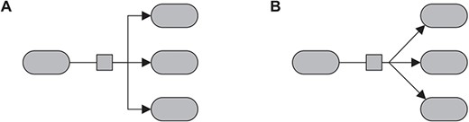
Different routing styles for edges. A. All edges are routed in an orthogonal style. B. All edges are routed as straight lines. Especially for short edges, straight-line routes may produce more readable results with fewer bends.
Embedding/orthogonalisation constraints to realize the desired angles around the process nodes
For the planarisation phase, we have to consider the following additional constraint: in the cyclic order of the edges around each process node, the incoming and outgoing edges (i.e. the consumption and production links) have to form separate, non-intersecting intervals. Based on our current planarisation approach that routes edges by means of a shortest-path search in the dual graph, this would only require minor changes. Furthermore, in order to realize the desired angles between the incoming/outgoing edges, we can use a similar approach [50] which allows specifying prescribed angles between consecutive edges around each node.
Place starting elements top/left
There is an extension of the TSM approach that allows placing each node inside a partition cell of a rectangular partition of the drawing area [51]. We could adopt a similar strategy to comply with the requirement that specific elements should be placed either at the top or left side of the drawing area. Note that this approach only restricts the starting elements to be placed above (or to the left) of the remaining elements. In order to obtain a uniform flow direction (e.g. from left to right), we could also consider the approaches described by Eiglsperger and co-authors [52].
Specific layout of cycles
In order to address requirement R3b, we aim at placing cycles that do not pass the bounds of a compartment on a convex/rectangular shape. Such a shape can be obtained by the same orthogonalisation strategy that is applied to compartments/clusters [46]. In addition, elements that do not belong to a cycle should be placed outside of it. Note that the flipping strategy described in the advanced approach A2c does not always guarantee this outcome, because it can only be applied to specific subcomponents. Hence, we can use the following approach to ensure this happens as expected: we propose to start by detecting the cycles and then temporarily grouping the associated elements into clusters. Hence, without any further changes to our existing approach that already supports clusters, the elements that do not belong to a cycle will always be placed outside of it.
Consideration of the mental map
A possible starting point for an approach that preserves the mental map is the definition and use of landmarks to orient a user. In the context of pathway layout, landmarks are distinguishable structures that relate to specific functionality and may be used as starting points in an approach preserving both appearance and relative organisation of certain structures across different maps. The user should thus be able to recognise these structures quickly and find pathway elements relative to the landmark structures without doing a full scan of the graph. Yuan et al. [53] describe an approach where subgraph layouts predefined by users are merged together to form a full layout of a graph. Such an approach could be adapted for biological pathways for which layouts of subgraph structures within pathways could be merged to maintain familiarity and relative position and act as landmarks in new pathway visualisations.
Conclusion
In this work, we provide an overview of graph drawing human-inspired requirements for pathway hypergraphs and explore some of these with an advanced layout algorithm to motivate further advances in the field. This overview is based on established graph drawing aesthetics as well as requirements specifically related to the SBGN process description specification but also human preference discovered through analysis and expert knowledge.
We demonstrate that it is possible to create satisfying layouts for process description diagrams and provide an enhanced algorithm that provides results close to manually drawn layouts for comparatively small signalling pathways made of up to 20 nodes. In particular, this algorithm takes into account packing and hierarchical nesting of complexes as well as flipping of sub-components outside of cyclic structures.
We believe that the growing demand for minimising the time-consuming manual work in the development of pathway-based detailed diagrams will catalyse new efforts and lead to new advanced solutions that may outperform the quality and aesthetics of human-drawn diagrams, especially for large networks. Systems Biology offers a diverse range of layout challenges, and many of the principles developed to address them can be generalised and will impact layout tasks in other domains.
The article outlines the requirements for producing a domain-specific layout for detailed signalling diagrams.
Currently, this task is predominantly realised by experts in a time-intensive effort. We demonstrate that it is possible to produce satisfying automatic layouts for comparatively small networks.
We offer suggestions for further developments within the emerging field of human-like layout algorithms.
Acknowledgements
This work was supported by yWorks GmbH and the LIST.
Funding
European Translational Information and Knowledge Management Services project of the Innovative Medicines Initiative (115446).
Availability
All relevant data are provided within the paper and Supplementary Materials. The yEd Graph Editor is a freely available tool (https://www.yworks.com/products/yed). The SBGN palette is supported in the yEd Graph Editor since version 3.17.1 and the enhanced layout algorithm since version 3.18.1. The translation between yEd GraphML and SBGN-ML is ensured by the open-source ySBGN application available at https://github.com/sbgn/ySBGN.
Martin Siebenhaller is a senior software developer at yWorks GmbH, working on the implementation and improvement of graph analysis and layout algorithms.
Sune S. Nielsen is a research and technology associate at the Environmental Informatics unit of the Luxembourg Institute of Science and Technology (LIST), working in the field of bioinformatics on graph visualisation and machine learning topics.
Fintan McGee is a researcher at the Environmental Informatics unit of the LIST. His current areas of research include biological pathway visualisation, multilayer network visualisation, as well as the evaluation of visualisation techniques.
Irina Balaur is a researcher at the European Institute for Systems Biology and Medicine (EISBM), working on network-based analysis within Systems Biology and on development of computational tools to facilitate management of heterogeneous biological information available in various standard formats.
Charles Auffray is the president and founding director of the EISBM. He develops a systems approach to complex diseases, integrating functional genomics, mathematical, physical and computational concepts and tools.
Alexander Mazein is a senior researcher at the EISBM, working on a comprehensive representation of disease mechanisms, complexity management and high-throughput biological data interpretation in translational medicine projects.
References
