


Abstract
The modelling of biological systems is accompanied with epistemic uncertainties that range from structural uncertainty to parametric uncertainty due to such limitations as insufficient understanding of the underlying mechanism and incomplete measurement data of a system. Fuzzy logic approaches such as fuzzy Petri nets (FPNs) are effective in addressing these issues. In this paper, we review FPNs that have been used for modelling uncertain biological systems, which we classify in three categories: basic fuzzy Petri nets, fuzzy quantitative Petri nets and Petri nets with fuzzy kinetic parameters. For each category of these FPNs, we summarize its modelling capabilities and current applications, discuss its merits and drawbacks and give suggestions for further research. This understanding on how to use FPNs for modelling uncertain biological systems will assist readers in selecting appropriate FPN classes for specific modelling circumstances. This review may also promote the extensive research and application of FPNs in the systems biology area.
Introduction
Systems biology [1, 2] aims to study the interactions between the components of a biological system and how these interactions cause the behaviour of the system as a whole. With the rapid development of high-throughput experimental technologies such as genomics and proteomics, modelling and simulation has become an essential approach in the study of systems biology by employing the data to build mathematical or computational models of a biological system, which help biologists to better understand and predict the system. Gradually, a picture of a biological system is emerging, which takes the form of a computational model with varying levels of details.
However, the complexity of biological systems gives rise to a number of modelling challenges, one of which is uncertainty [3]. Uncertainties generally fall into two categories: aleatoric and epistemic [4]. Aleatoric uncertainty usually stems from intrinsic internal noise of a (biological) system [5] that follows some physical principles and has to be addressed by stochastic methods such as stochastic differential equations, Markov chains or stochastic Petri nets (SPNs) [6]. Epistemic uncertainty usually results from the lack of knowledge of the (biological) system to be studied due to such limitations as insufficient understanding of the mechanisms underlying the system, incomplete measurement data for some components or measurement errors for some data. This kind of uncertainty is in its very nature different from the former one and is appropriately dealt with using fuzzy techniques [7] rather than stochastic ones.
![(a) Two definitions of the set of ‘comfortable temperatures’ on a universe of all real numbers $\mathbb {X}$. The classical (crisp) set defines it as [20, 24], indicating a temperature value $x$ belonging to this interval means comfortable, i.e. $\mu (x)=1$; otherwise not, i.e. $\mu (x)=0$. The TFN, $S= (12, 22, 32)$ as a special fuzzy set, defines the set of ‘comfortable temperatures’ in a more natural way, by giving the degree of membership of each temperature value $x$, i.e. $\mu (x)\in [0,1]$. This definition considers the diversity of how different people feel comfortable about distinct temperature. (b) Illustration of the $\alpha $-cut. The $\alpha $-cuts for $\alpha =0.5$, $\alpha =0.8$ and $\alpha =1.0$ are calculated as crisp subsets $[17,27]$, $[20,24]$ and $\{22\}$, respectively. (c) The main elements of an FIS. Crisp input values are converted via the fuzzifier into fuzzy values, which are then fed into the inference engine. The inference engine performs the reasoning with the fuzzy rules in the rule base and produces fuzzy output values. The defuzzifier then converts the fuzzy output values into crisp output values.](https://oup.silverchair-cdn.com/oup/backfile/Content_public/Journal/bib/21/1/10.1093_bib_bby118/4/m_bby118f1.jpeg?Expires=1749194493&Signature=RJ5GiQaohlA2q5dZ9VnMpgKmfmR9~~uclvQWS73y3QAm1OMqR8CPDviCwS9N8-e~P7yfF3EbOOjS-oU~crwkEMr~UbwVv7bv8mXtqtNh95YfYmJFSVi4mk0y3lRJXqXH~EuzDwAle8kLy5WqEB-GLrhT1OFlgSuwt7ravke-eSBV6OoMnpowZz4m0PqH385KG2RPispedOjR3ocRlJm2O6lA2JxQtMKDk4l7OL8DWWVoWT~qZ2bj1TsgKdIHx4mQQS6E3wyGuObyMqBgtg1UckWLN0WQ5xJFrUOLgfB3n5zt-bt14XhNHR97BckR2FZ1KXaSJCQtgmmYiXzE2j~zxg__&Key-Pair-Id=APKAIE5G5CRDK6RD3PGA)
(a) Two definitions of the set of ‘comfortable temperatures’ on a universe of all real numbers |$\mathbb {X}$|. The classical (crisp) set defines it as [20, 24], indicating a temperature value |$x$ | belonging to this interval means comfortable, i.e. |$\mu (x)=1$|; otherwise not, i.e. |$\mu (x)=0$|. The TFN, |$S= (12, 22, 32)$| as a special fuzzy set, defines the set of ‘comfortable temperatures’ in a more natural way, by giving the degree of membership of each temperature value |$x$|, i.e. |$\mu (x)\in [0,1]$|. This definition considers the diversity of how different people feel comfortable about distinct temperature. (b) Illustration of the |$\alpha $|-cut. The |$\alpha $|-cuts for |$\alpha =0.5$|, |$\alpha =0.8$| and |$\alpha =1.0$| are calculated as crisp subsets |$[17,27]$|, |$[20,24]$| and |$\{22\}$|, respectively. (c) The main elements of an FIS. Crisp input values are converted via the fuzzifier into fuzzy values, which are then fed into the inference engine. The inference engine performs the reasoning with the fuzzy rules in the rule base and produces fuzzy output values. The defuzzifier then converts the fuzzy output values into crisp output values.
A (biological) model can be simply represented as a tuple |$(F,\theta )$|, where |$F$| and |$\theta $| denote the structure and parameters of the model, respectively [8]. To build a model means to determine these two artefacts. The gap between |$(F,\theta )$| and the unknowable true system that the model represents constitutes the structural uncertainty and parametric uncertainty, both of which belong to the epistemic uncertainty class and do exist in a biological model. When we have to deal with insufficient understanding of the mechanism or cannot obtain sufficient data of the system, we usually face structural uncertainty, i.e. it is hard to determine the exact structure of the model to be built. Furthermore, even if we are able to determine the model structure, we still have the parametric uncertainty issue due to incomplete or erroneous measurement data. These two kinds of uncertainties make biological systems uncertain and complicate the modelling and analysis of biological systems. Fortunately, fuzzy logic offers an effective approach to address these two issues.
Fuzzy logic, first proposed by Zadeh [9], offers a computational tool to deal with vague, ambiguous, noisy or imprecise information by simulating human reasoning and natural language. Fuzzy logic uses the degree of belonging defined by a membership function to describe an element, and thus can represent uncertainties in a computational model. Fuzzy logic has been widely used in different areas including systems biology [10, 11]. Generally, the use of fuzzy logic requires one to write a set of fuzzy rules for a system to be examined, constituting a fuzzy rule model, which becomes hard to be managed with increasing numbers of fuzzy rules.
To facilitate the use of fuzzy rules, fuzzy Petri nets (FPNs) [12, 13] have been designed by combining fuzzy logic and Petri nets (PNs), which offer a graphical representation of fuzzy rules, making it easier for biologists to work with fuzzy rules. Likewise, FPNs have been deployed for many applications [14] including systems biology (see, e.g. [15, 16]). Starting from basic FPNs, where an FPN model can be considered to be equivalent to a set of fuzzy rules [12, 13], many extensions have been proposed, such as fuzzy hybrid functional Petri nets (FHFPNs) [16], continuous/stochastic Petri nets with fuzzy kinetic parameters (CPN-FPs/SPN-FPs) [17, 18] and fuzzy timed Petri nets [19]. Different kinds of FPNs play different roles in the modelling of a biological system, either building a fuzzy model of the whole system [15] or building a hybrid model with some components being fuzzy ones and others being quantitative ones [16], or building a quantitative model that only allows kinetic parameters to be fuzzy [17, 18].
However, although FPNs are very attractive and powerful to deal with a wide range of uncertainty issues in systems biology, they have not been extensively applied in this area so far. In this paper, we review three kinds of FPNs that have been used for modelling of biological systems, and we explore how they address structural uncertainty and parametric uncertainty in biological systems. We also summarize the applications of different FPN approaches in systems biology and discuss possible further research directions. We hope this review will open a door for the wide application of FPNs in the systems biology area.
Fuzzy logic & Petri nets
Fuzzy logic
The fundamental concept of fuzzy logic is the fuzzy set [9]. Let us assume a universal set |$\mathbb {X}$| and a membership function |$\mu $| that specifies for each element of the universal set the membership in a given subset |$S \subseteq X$|. For classical (crisp) sets, this membership function only takes the Boolean values 0 or 1, i.e. an element of the universal set either belongs to |$S$| or it does not belong to |$S$|. In contrast, for fuzzy sets, this membership function takes real values in the closed (unit) interval [0, 1], defining a membership degree for each element of the universal set.
A fuzzy number is a special (convex and normalized) fuzzy set with the universal set given by the set of real numbers. Commonly used fuzzy numbers include triangular, trapezoidal and Gaussian fuzzy numbers. For illustration, we consider triangular fuzzy numbers (TFNs), which are defined by triangularly shaped membership functions each specified by a triple |$(a,b,c)$|, |$a \leq b \leq c$|, where if |$a\leq x \leq b$|, |$\mu (x)=(x-a)/(b-a)$|; if |$b\leq x \leq c$|, |$\mu (x)=(c-x)/(c-b)$|; otherwise, |$\mu (x)=0$|. Figure 1a illustrates the difference between classical sets and fuzzy sets. The |$\alpha $|-cut of a fuzzy set |$\tilde {S}$| at a given membership degree |$\alpha \in [0,1]$| (formally called |$\alpha $| level), denoted by |$\tilde {S}_{\alpha }$|, consists of a crisp subset of |$\mathbb {X}$|, in which each element has a membership degree greater than or equal to the given |$\alpha $| level. The |$\alpha $|-cut of a TFN is computed as follows: |$\tilde {S}_{\alpha }=[a + \alpha (b - a), c - \alpha (c - b)]$|; see Figure 1b for an example.
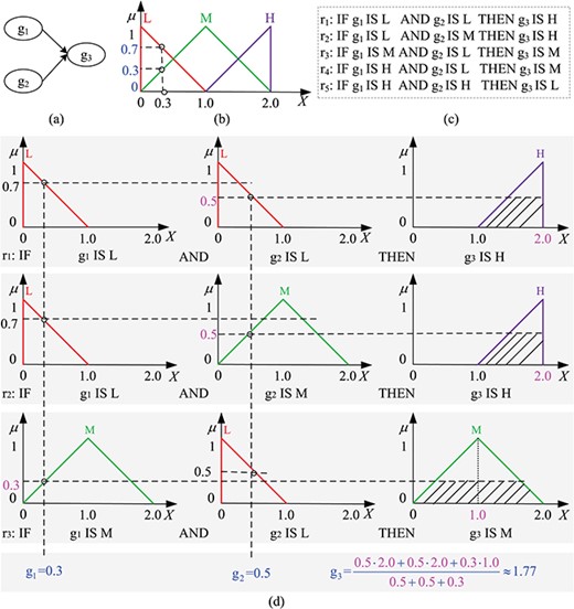
A fuzzy inference system example. (a) A three-gene network, which is used to study how two genes, g|${}_1$| and g|${}_2$|, affect another gene, g|${}_3$|. (b) The membership functions of three linguistic terms: L (Low, red), M (Medium, green) and H (High, purple), each being associated with a TFN. Each gene could have a different linguistic term set; in this example we use the same linguistic terms for the three genes. We assume the expression level of each gene ranges from 0 to 2. A crisp expression level of any gene, e.g. 0.3, is converted to a fuzzy value, (0.7,0.3,0), which means that the membership degrees of the value 0.3 belonging to L, M and H are 0.7, 0.3 and 0, respectively, i.e. |${{\mu } _{\text {L}}}(0.3)=0.7$|, |${{\mu } _{\text {M}}}(0.3)=0.3$| and |${{\mu } _{\text {H}}}(0.3)=0$|. (c) The user-defined fuzzy rules for the three-gene network forming the FIS rule base. (d) A complete reasoning process of the example; g|${}_1=0.3$| and g|${}_2=0.5$| yield g|${}_3=1.77$|.
There are two popular ways to apply fuzzy logic. One is to divide a fuzzy set into a number of |$\alpha $|-cuts and then to adopt Zadeh’s extension principle to generate the membership function of each output according to the membership functions of all inputs [20]. The crucial ideas underlying this approach will be discussed in Quantitative PNs with fuzzy kinetic parameters section. Another way to apply fuzzy logic is to use fuzzy sets representing linguistic terms to describe the states of a system, fuzzy rules to represent the transition of the states and a fuzzy inference system (FIS) to reason the evolution of the system.
An FIS is a system that maps inputs to outputs using fuzzy logic [21]. It consists of four main components: fuzzifier, rule base, inference engine and defuzzifier (see Figure 1c). Figure 2 gives an example to demonstrate how an FIS works. The example considers a three-gene network, which we use to analyse how two genes, g|${}_1$| and g|${}_2$|, affect another gene, g|${}_3$| (see Figure 2c). We define three linguistic terms, L (Low), M (Medium) and H (High), to describe the expression levels of these genes. Each linguistic term is associated with a TFN (see Figure 2b). In theory, more linguistic terms mean a more accurate description of a system, which, however, would cause higher computational costs. Therefore, in practice, we usually choose a smaller odd number of terms like 3, 5 or 7 in order to have a midpoint value. We then construct a set of fuzzy rules (Figure 2c) to describe how the expression levels of genes g|${}_1$| and g|${}_2$| affect the expression level of g|${}_3$|.
In an FIS, the fuzzifier converts a crisp input value to a fuzzy value by computing the membership degree for each of the defined linguistic terms. For example, a crisp value 0.3 is converted to a fuzzy value (0.7, 0.3, 0), which means that the membership degrees of the value 0.3 belonging to L, M and H are 0.7, 0.3 and 0, respectively, i.e. |${{\mu } _{\text {L}}}(0.3)=0.7$|, |${{\mu } _{\text {M}}}(0.3)=0.3$| and |${{\mu } _{\text {H}}}(0.3)=0$| (see Figure 2b for illustration).
Fuzzy logic belongs to the logic modelling category [22]. Logic models were proposed to address the limitations of quantitative models due to the lack of experimental data and thus lack of precise kinetic parameters. Boolean networks, in which each variable takes only two values, 0 or 1, and the reasoning is based on Boolean logic, offer the simplest logic models. The extension of Boolean networks to multi-valued variables allows the encoding of much richer behaviours of biological systems. Fuzzy logic ultimately achieves continuous regulations of variables in logic models by representing the knowledge with a gradual degree of membership (in the interval [0,1]) instead of crisp membership (0 or 1) allowed in Boolean logic. In summary, fuzzy logic offers more accurate and natural representations of biological systems than Boolean networks; for more discussions see [22, 23].
There are a couple of advantages of using fuzzy logic for modelling and inferring biological systems. For example, fuzzy logic inherently accounts for noise in the data and allows for imprecise values, and thus fuzzy logic models tend to be more robust. Fuzzy logic allows the fusion of high-level, human-like reasoning in modelling and inferring biological systems; therefore, it is advantageous for biologists to construct biological models with their rich knowledge in an intuitive fashion using fuzzy logic. Moreover, if experimental data are available, it is easy to infer the underlying causal mechanisms of a biological system with fuzzy logic. In fact, this topic has attracted many researchers. A typical inferring approach with fuzzy logic was proposed by Woolf et al. [24]. They designed a triplet model, consisting of an activator, a repressor (both are inputs) and a target (output), and used fuzzy rules to describe their relationships. Each time, they arbitrarily selected and assigned three genes (a gene combination) to the triplet model and then ran the model with the expression values of the activator and repressor, producing predictions of the target. They then assigned a rank to the gene combinations in terms of the error between the prediction values and its measurement values of the target. Finally, they found out those combinations that had a low prediction error, which most likely represented the relationships among triples of genes.
Petri nets
Petri nets [25] are an excellent modelling formalism for describing and studying many different types of systems especially characterized as being concurrent, asynchronous, distributed, parallel or nondeterministic. The formalism combines an intuitive graphical notation with a number of advanced analysis techniques with a firm mathematical foundation. PNs are applied in practice by industry, academia and other fields to the analysis of systems arising in asynchronous circuit design, communication protocols, distributed computing, production systems, flexible manufacturing, transportation, systems biology, etc. [25, 26]. PNs are directed, bipartite multigraphs, consisting of places, transitions and weighted arcs that connect them. In systems biology, places usually represent species or any kind of chemical compounds, e.g. genes, proteins or protein complexes, while transitions represent any kind of chemical reactions, e.g. association, disassociation, translation or transcription. Based on standard (qualitative) PNs, many extensions, e.g. stochastic Petri nets (SPNs), continuous Petri nets (CPNs) and coloured (stochastic, continuous) Petri nets (ColPNs) [27], have been proposed for modelling and simulating biological systems [26]. Among them, SPNs and CPNs are classified into the quantitative PN category. We will introduce them in more detail in the following sections when they are used.
Combining Petri nets with fuzzy logic
Fuzzy logic has been combined with many other methods, such as Petri nets, artificial neural networks, differential equations and cognitive maps, to take advantage of the synergy between graphical representation capability and uncertainty handling capability [21]. Among those combinations, fuzzy Petri nets (FPNs) have a long tradition; see [28] for an early mini review illustrating the use of FPNs for discrete event dynamic systems, such as manufacturing systems. In our paper, the focus will be on the application of FPNs in systems biology. So far, there have been several ways proposed to achieve a combination of PNs with fuzzy logic specifically dedicated for the use in systems biology, which we summarize as follows (see Figure 3).
i. Graphical elements of PNs represent fuzzy rules [13]. We call this combination basic fuzzy Petri nets (BFPNs). In fact, most FPNs in the literature apply BFPNs. In this case, a BFPN is equivalent to a set of fuzzy rules. Therefore, BFPNs can address the uncertainty of the model structure when the system under study suffers from insufficient prior knowledge or measurement data to capture its accurate structure.
ii. Fuzzy quantitative Petri nets (FQPNs) combine fuzzy rules with quantitative Petri nets [16]. In such an approach, fuzzy rules and quantitative Petri nets describe different parts of a system, which communicate via specially designed interfaces (information interaction). A model built with this approach comprises some uncertain (fuzzy) components and some certain components, depending on the availability of data.
iii. Petri nets with fuzzy kinetic parameters, e.g. CPN-FPs and SPN-FPs [17, 18]. Such a model is basically a quantitative model (either a CPN or SPN), but kinetic parameters are allowed to be fuzzy numbers. Thus, this combination allows for models that are less uncertain compared with BFPNs and FQPNs.
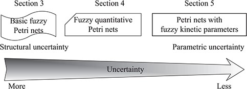
Spectrum of fuzzy Petri nets, reflecting the uncertainty degree of models built with different approaches, from structural (more) to parametric (less) uncertainty. The choice among these modelling approaches depends on prior knowledge about the biologic system to be studied and the quality and availability of experimental data.
Figure 3 illustrates how these three FPN approaches address different types of uncertainties ranging from structural to parametric uncertainties in biological systems. The choice among these modelling approaches depends on prior knowledge about the biologic system to be studied and the quality and availability of experimental data, etc.
In the next three sections, we will in detail review each of these approaches and their applications in systems biology, complemented by a brief summary. We will discuss these three approaches in the order in which uncertainties decrease, i.e. from structural to parametric uncertainties.
Basic fuzzy Petri nets
FPNs [13, 29] were first proposed in the knowledge representation area to facilitate the use of fuzzy rules by making use of the graphical elements of PNs. Therefore, FPNs can graphically represent fuzzy rules and use fuzzy reasoning to explain the behaviour of a system. FPNs have been applied to various areas such as fault diagnosis [14]. So far, many types of FPNs have been proposed, depending on the fuzzy reasoning algorithms they use and the model representation capabilities they offer [14]. Among them, FPNs that combine PNs and fuzzy logic are the most used ones, which we call basic fuzzy Petri nets (BFPNs) in this paper. See Figure 4 for an example, which represents the fuzzy rules given in Figure 2.
![(a) A BFPN example, which represents the fuzzy rules given in Figure 2c. Each place represents a proposition, given on the right side as a comment; each transition represents a rule, i.e. r${}_i$ corresponds to the rule r${}_i$, where $i$= 1,2,...,5. (b) A coloured version of the BFPN model, where each coloured place folds three uncoloured places, e.g. place g${}_1$ folds places g${}_{1\text {L}}$ to g${}_{1\text {H}}$, by using a colour set with three colours (see the right side for declarations). The guard function helps distinguish the five uncoloured transitions as they are folded into one coloured transition cr. The variables, x, y and z, associated with the arcs specify the flow of tokens of appropriate colours. See [38] for the detailed syntax of colour-related declarations.](https://oup.silverchair-cdn.com/oup/backfile/Content_public/Journal/bib/21/1/10.1093_bib_bby118/4/m_bby118f4.jpeg?Expires=1749194493&Signature=uN7CFUlS1g1UjVKZMiPEJJL3CcK-aI~vGo5kKw5myGtoEc9QREnj~jK6tlFpU6phhf7udUD4neIjNWvkdFdvrYv0i2-uywAhkQbyC0dvtEXiinkKPi1guC5l~l5BLATXMybYlmiWoKeQ1mQOnctYdFvPIWkdLoAJUbC624gvGvekttsPWQE5~RG1XvCjmbsoRUWHKt9CuJJHMc1EA1johV~hwUxNzwCklKnEjEuIduKsc-LvntmC93CNjEl8QLw5SKo8KGaC8z36Z0qA0VI6ok39YvQA7ZMnoOuIu7lhCLoCrRZqX7UsoJiEH6K-KdjkBICvclPXHPG8GCWY~vTmCw__&Key-Pair-Id=APKAIE5G5CRDK6RD3PGA)
(a) A BFPN example, which represents the fuzzy rules given in Figure 2c. Each place represents a proposition, given on the right side as a comment; each transition represents a rule, i.e. r|${}_i$| corresponds to the rule r|${}_i$|, where |$i$|= 1,2,...,5. (b) A coloured version of the BFPN model, where each coloured place folds three uncoloured places, e.g. place g|${}_1$| folds places g|${}_{1\text {L}}$| to g|${}_{1\text {H}}$|, by using a colour set with three colours (see the right side for declarations). The guard function helps distinguish the five uncoloured transitions as they are folded into one coloured transition cr. The variables, x, y and z, associated with the arcs specify the flow of tokens of appropriate colours. See [38] for the detailed syntax of colour-related declarations.
Like Petri nets, BFPNs are also directed, bipartite multigraphs, consisting of places, transitions and arcs. However, in a BFPN, places do not represent such passive elements as objects and states, but propositions, while transitions represent fuzzy rules over these propositions. For example, in Figure 4a, place g|${}_{1\text {_L}}$| represents the proposition ‘g|${}_1$| IS L’, g|${}_{2\text {_L}}$| ‘g|${}_2$| IS L’ and g|${}_{3\text {_H}}$| ‘g|${}_3$| IS H’. Transition r|${}_1$| represents the rule r|${}_1$|: ‘IF g|${}_1$| IS L AND g|${}_2$| IS L THEN g|${}_3$| IS H.’ Directed edges represent the direction of the reasoning. Each place p, which represents a proposition, gets a truth degree (or membership degree) |$\mu _{\text {p}}$| in [0,1], obtained via fuzzification of a given crisp value of a species like g|${}_1$|. Tokens on places hold membership degrees, which are propagated level by level while applying the rules. There is no conflict in a BFPN, which means that all transitions sharing a preplace can fire concurrently. In a biological scenario, we usually do not allow the association of a certainty factor and threshold with a transition. Therefore, a BFPN is usually equivalent to an FIS; however, a BFPN also allows cascaded fuzzy rules, which result in cascaded FISs [30]. This means, BFPNs are more powerful than FISs in terms of the representation capability by allowing both single level and cascaded fuzzy rules.
According to [13], there are three commonly used types of fuzzy rules. The corresponding PN of each type of rules is given in [31]. When constructing a biological model with BFPNs, we can use the following rules as basic components and form larger ones in a bottom-up way.
i. |$r_k$|: |$p_1(\mu _1)$| AND |$p_2(\mu _2)$| AND... AND |$p_{M-1}(\mu _{M-1})$||$\rightarrow p_{M}(\mu _{M})$|, where |$\mu _{M} = \text {min}\{\mu _1, \mu _2,..., \mu _{M}\}$|.
ii. |$r_k$|: |$p_1(\mu _1)$||$\rightarrow $||$p_2(\mu _2)$| AND... AND |$p_{M-1}(\mu _{M-1})$| AND |$p_{M}(\mu _{M})$|,where |$\mu _{j} = \mu _1$|, |$j=2,3,...,M$|.
iii. |$r_k$|: |$p_1(\mu _1)$| OR |$p_2(\mu _2)$| OR... OR |$p_{M-1}(\mu _{M-1})$||$\rightarrow p_{M}(\mu _{M})$|, where |$\mu _{M} = \text {max}\{\mu _1, \mu _2,..., \mu _{M}\}$|.
If we have a BFPN model ready, we can employ a specific reasoning algorithm to execute or simulate it. So far, there have been many reasoning algorithms proposed, each of which is developed for and thus adapts to a specific application scenario or problem. In the systems biology scenario, we have to carefully choose appropriate reasoning algorithms. For instance, [31] gives a reasoning algorithm appropriate for biological systems, which implements the reasoning of cascaded FISs and works as follows. In the fuzzification phase, it computes the truth degree (or membership degree) of each place (corresponding to a proposition) by fuzzifying the crisp value of a species, e.g. g|${}_1$| or g|${}_2$| in Figure 4a. It then starts parallel reasoning from the first level to produce new truth values for the next level, which is repeated until the last level. In the defuzzification phase, it defuzzifies the fuzzy values to obtain a crisp value for each species. This algorithm has been demonstrated and validated in [31].
Furthermore, coloured fuzzy Petri nets (ColFPNs) [31] were proposed to deal with biological systems by combining BFPNs with coloured Petri nets (ColPNs). ColPNs, as a parameterized modelling method, can represent a large-scale system as a compact model by encoding similar components of the system as colours. In a ColFPN (see Figure 4b for an example), a group of propositions related to a species is encoded as a set of colours, forming a colour set. All the propositions in a group are represented as a coloured place, and each proposition is distinguished by a specific colour. For example, in Figure 4b, a colour set CS is defined to have three linguistic terms, L, M and H, as colours, and each colour (e.g. L) associated with a place (e.g. g|${}_1$|) represents a proposition (e.g. g|${}_1$| IS L). Likewise, a group of fuzzy rules is represented as a coloured transition with a guard and distinguished with colours. The variables on arcs (e.g. three variables, x, y and z are declared in Figure 4b) specify the flow of appropriate colours. For example, a guard, guard(x,y,z), is defined in Figure 4b to distinguish each of the five rules. A value combination [e.g. (L,L,L)] for (x,y,z), with which the guard is evaluated to true, represents a legal rule. This offers an approach to conveniently represent a large number of fuzzy rules with a compact ColFPN model, whose size is substantially decreased compared with its corresponding BFPN model. In fact, ColFPNs significantly improve the model readability, although their simulation complexity remains basically unchanged or is even slightly worse due to the introduction of an unfolding step before simulating, which, however, can be neglected for even large models thanks to sophisticated unfolding algorithms, such as the constraint satisfaction approach [32]. The simulation of a ColFPN model is divided into two steps. It first implicitly unfolds a ColFPN model to a BFPN model and then adopts the same reasoning algorithm as that for BFPNs.
Applications
Hamed et al. [33] presented a BFPN model of a genetic regulatory network (GRN) with three genes and proposed a reasoning algorithm to automatically reason about imprecise and fuzzy information in GRNs. They illustrated in detail the computation of each step with this model, and their work can be considered as a good tutorial for the use of BFPNs for the modelling of biological systems. Besides, they used Matlab [34] to implement their algorithm and model; however, Matlab does not easily support cascaded FISs and is not easy to use for biologists. Further, they gave an illustrative BFPN model of GRNs in [35], which considers the regulatory triplets by means of predicting changes in the expression level of the target based on the input expression level. These two works are early attempts to use FPNs for modelling biological systems.
Küffner et al. [36] presented a network inference approach based on Petri nets with fuzzy logic (PNFL), which can also be considered as a kind of BFPN. In contrast to the BFPNs above, in a PNFL model, places are divided into effector and target ones, the arcs between that are called effect arcs. If several effectors regulate a target gene, their combined effect on the target is described by logical operations such as the AND or OR operators. They also considered some parameters like effect strength. They then developed a PNFL simulation algorithm to dynamically run their models. They inferred and constructed a PNFL model in the following way: (1) randomly initialize the topology and parameters of the model for a couple of genes; (2) the model is simulated to produce the prediction values of the target; (3) by comparing the prediction values with measurement values of the target, an objective function is computed. According to the objective function, the model topology or parameters are changed, e.g. adding or removing effect arcs, switching the effect combination logic operators, increasing or decreasing the effector strength. By repeating the steps above, the model that matches the experimental data is finally obtained. It has been shown that their approach correctly reconstructed networks with cycles as well as oscillating network motifs. In addition, they built a minimal model of a Higgins–Sel’kov oscillator using PNFL in [37]. However, these works above only consider a single level of fuzzy rules and do not really show the power of BFPNs.
Liu et al. [17] presented a ColFPN approach for modelling and analysing biological systems to deal with large networks with many fuzzy rules in a parameterized way. They illustrated their approach by developing a ColFPN model of a GRN with 6 genes and 24 fuzzy rules. This model has three levels of fuzzy rules, consisting of cascaded FISs. It has been shown that the model’s readability is significantly improved with ColFPNs, and the ColFPN model retains the original structure of the GRN (compare Figure 4a and b for another example). Also, they proposed a fuzzy reasoning algorithm that is applicable for analysing biological systems. This algorithm performs parallel reasoning based on matrix operations for large biological models. They developed their models using an internal version of Snoopy [38], which are then simulated using Matlab.
A brief summary
As seen from the applications above, the use of BFPNs for systems biology is not extensive at this moment, and the size of the BFPN models that can be considered is basically small, although [17] gives a relatively large model and a promising approach to constructing larger models. This might be caused by the lack of appropriate algorithms and powerful tools.
As described above, each fuzzy reasoning algorithm has been developed for a specific area, thus we need to carefully develop an appropriate one for systems biology. BFPNs support cascaded fuzzy rules (cascades FISs), which are more powerful than usual fuzzy toolboxes such as the FIS component in Matlab, which only supports a single level of fuzzy rules (one FIS). Thus, the (fuzzy) Petri net modelling community (shortly the community in the following) needs to focus on the development of reasoning algorithms for cascaded FISs in a next step, as was done in [17].
On the other hand, at present, most applications of BFPNs in systems biology (and many other areas) are based on Matlab. That is, they use Matlab (Simulink) to model and analyse BFPNs. However, this has many drawbacks. For example, it does not easily support cascaded FISs, and the interface is not user-friendly. In contrast, biologists often prefer to use a simple graphical tool. This is also the reason why PNs, supported by many easy-to-use tools, are widely used in this area. Therefore, the development of a simple graphical tool for BFPNs could be a good option. In summary, in the future the community should strengthen the research of at least these two aspects in order to promote the further application of BFPNs in systems biology.
Fuzzy quantitative Petri nets
What we mean by fuzzy quantitative Petri nets (FQPNs) is a combination of fuzzy logic with a kind of quantitative Petri nets, which aims to complement uncertain modelling capabilities for existing quantitative PNs. FQPNs offer a semi-quantitative approach to modelling a complex biological system, where some components can be built as uncertain fuzzy models if kinetic data are not available or insufficient and the others as certain ones if kinetic data are sufficient. Currently, there are two kinds of FQPNs that have been proposed for systems biology.
One is fuzzy hybrid functional Petri nets (FHFPNs), proposed by Windhager in [16], which are considered as an instance of hybrid functional Petri nets (HFPNs) [39] by extending HFPNs with fuzzy logic. An HFPN has two kinds of places (transitions): discrete and continuous and allows the weight of each arc to be a function over its preplaces. Thus, an HFPN model can be divided into two parts, discrete and continuous. The former can model discrete quantities like molecular numbers or concentration levels and how they transit from one state to another, and the latter can model continuous quantities like concentration of species and how they evolve continuously. Unlike HFPNs, in an FHFPN, the weight of an arc is allowed to be an FIS, besides other forms of functions that are allowed in HFPNs. See Figure 5 for an illustrative example, which models the following scenario. Genes g|${}_1$| and g|${}_2$| produce proteins p|${}_1$| and p|${}_2$|, respectively; gene g|${}_3$|, positively regulated by p|${}_1$| and p|${}_2$|, produces p|${}_3$|. Each species is modelled as a continuous place and each biological reaction as a continuous transition. The concentration increase of p|${}_3$| is computed via an FIS by setting the weight of the arc from r|${}_3$| to p|${}_3$| to ‘0.2 + FIS(g|${}_3$|,p|${}_1$|,p|${}_2$|;p|${}_3$|)’. The weights of the other arcs are either a real number or a function of preplaces (e.g. |$0.7 \cdot \text {g}_2$|). The model can be divided into two parts: the uncertain one (in the dashed frame), which follows an FIS semantics, and the certain one (outside the dashed frame), which follows the semantics of HFPNs.
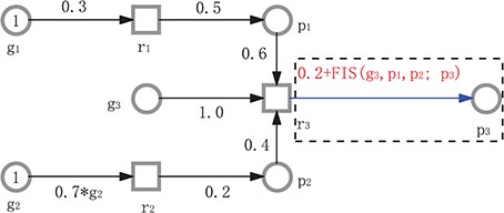
An FHFPN example. In this model, the weight of the arc from r|${}_3$| to p|${}_3$| is set to a fuzzy expression, 0.2 + FIS(g|${}_3$|,p|${}_1$|,p|${}_2$|;p|${}_3$|), where we use a semicolon to separate the input and output of the FISand a comma to separate each input variable, while the others are crisp expressions. This model can be divided into two parts: the uncertain one (in the dashed frame), which follows an FIS semantics, and the certain one (outside the dashed frame), which follows the semantics of HFPNs. All rate functions (not given) follow mass action kinetics.
The simulation of an FHFPN model can adopt different firing rules as given in [16]: (1) random firing, in which transitions are randomly chosen, one by one; (2) stochastic firing, in which transitions are chosen using the Gillespie stochastic simulation algorithm [40]; and (3) simultaneous firing, in which the marking is updated when all transitions have fired. Although these rules were given in [16], the 2nd one has never been found to be applied in any example so far.
Another class of FQPNs is fuzzy continuous Petri nets (FCPNs), proposed by Bordon et al. in [41], which extend CPNs given in [42] with fuzzy logic. CPNs offer a graphical way to represent systems of ordinary differential equations (ODEs) [43]. In a CPN model, places take real-valued tokens to represent the concentration of species, while transitions represent continuous changes of concentrations. When simulating a CPN model, we first convert its graphical representation to a set of ODEs and then adopt suitable numerical ODE solver to obtain simulation results.
In contrast, in an FCPN some transitions are allowed to be fuzzy ones and the others are continuous ones that are equivalent to a set of ODEs, as a CPN does. Each fuzzy transition is considered as an FIS, which calculates a concentration change per time step of a specific species in a fuzzy way. See Figure 6 for an illustrative example, which models almost the same scenario as that in Figure 5. In this model, transition t|${}_3$| is modelled as a fuzzy transition, taking a fuzzy rate, FIS(g|${}_3$|,p|${}_1$|,p|${}_2$|;p|${}_3$|), which computes the concentration change of p|${}_3$| via an FIS. Similarly, the model can be divided into two parts: the uncertain one (consisting of transition t|${}_3$| and place p|${}_3$|), which follows an FIS semantics, and the certain one (the other places and transitons), which follows the semantics of ODEs. Besides, in order not to affect other places, all the input places of the fuzzy transition are connected with read arcs. A read arc allows one to model that some resource is required but not consumed upon firing [38].
![An FCPN example, which has a special fuzzy transition r${}_3$ with the rate, FIS(g${}_3$,p${}_1$,p${}_2$;p${}_3$). That is, the concentration change of p${}_3$ is calculated in terms of the concentrations of g${}_3$, p${}_1$ and p${}_2$ via the FIS, while the others are computed via an ODE solver. The arcs with a filled circle are read arcs. A read arc allows one to model that some resource is required but not consumed upon firing [38]. All rate functions (not given) follow mass action kinetics.](https://oup.silverchair-cdn.com/oup/backfile/Content_public/Journal/bib/21/1/10.1093_bib_bby118/4/m_bby118f6.jpeg?Expires=1749194493&Signature=bLMkjFdAWDrqs-ml1sQ5CRg2GwOfKWSDK2M7u9IpC~UI~~p~75FwEMs29t1YpmcSqh1FM85gcxL4bQnSPHfml1dSvM9zipKJxKNrgRqHMZiqnH8xhVlN1uqo5yMzq8pfc0SE91pRjN7PNOQOaVP~~Eei01F2kQVFQJ5FnlfyyrvNue4rMuBw0sVs0eSRBYbxzGO6CkRJYVzM5VSqCbUVOn9LaEeKPp9gTnHRoPiW0D68errINy6~twd3PQ-nKh1CEB3QO~Kc1gPvAy2jCoi7QIMopWEMqmRX7XnP637hXKT0uNrz8ZGqoJOT3rWOzfzQ9DgdO3oU46fzdMTsgMkd3g__&Key-Pair-Id=APKAIE5G5CRDK6RD3PGA)
An FCPN example, which has a special fuzzy transition r|${}_3$| with the rate, FIS(g|${}_3$|,p|${}_1$|,p|${}_2$|;p|${}_3$|). That is, the concentration change of p|${}_3$| is calculated in terms of the concentrations of g|${}_3$|, p|${}_1$| and p|${}_2$| via the FIS, while the others are computed via an ODE solver. The arcs with a filled circle are read arcs. A read arc allows one to model that some resource is required but not consumed upon firing [38]. All rate functions (not given) follow mass action kinetics.
The simulation of an FCPN is performed in the following way. At each time step, evaluate each (continuous or fuzzy) transition, whether it is enabled. If yes, fire each continuous transition in the same way as for CPNs, and fire each fuzzy transition in the following steps: (1) fuzzify the given input species from crisp to fuzzy values, (2) calculate the fuzzy concentration change of output species via the inference engine by applying fuzzy rules and (3) defuzzify fuzzy values to crisp ones. Then update the concentration of each place according to the concentration changes resulting from different sources.
The differences of the two kinds of FQPNs given above lie in the following two aspects.
The position to hold an FIS is different. In an FHFPN, an FIS is allowed to occur in the weight of an arc, and moreover, a weight can be a function composed of constants and FISs, while in an FCPN, an FIS is associated with a transition, not an arc. Therefore, FHFPNs are more flexible and powerful than FCPNs in terms of the fuzzy capability. However, these two kinds of FQPNs can be converted into each other in the uncertain part.
The semantics of the certain part of these two FQPNs is different. That is, the certain part of an FHFPN adopts the semantics of HFPNs, while an FCPN adopts the semantics of ODEs.
Applications
Windhager [16] discussed the application of FHFPNs to several well-studied biological network motifs, including feed-forward loop, negative feedback oscillator, positive feedback toggle switch and positive feedback one-way switch. These examples showed that FHFPNs are appropriate to simulate these common network motifs.
Windhager [16, 44] further gave an FHFPN example, which models a simple biological system: green fluorescent protein (GFP) expression in a cell-free in vitro transcription/translation system. This model considers five species: Plasmids, mRNA, transcription resources (TsR), translation resources (TIR) and GFP. The change of the concentration of each species is computed with an FIS, and the weights of the other arcs are set to 0. He also developed an ODE model for this biological system and compared these two models, which indicated that the predictions of the FHFPN model are sufficient for hypotheses testing, if the experimental observations exhibit the qualitative different behaviour. In summary, the Windhager’s PhD thesis [16] offers an introductory description of FHFPNs and their application in biological systems. However, many issues have not been addressed, e.g. a precise definition of FHFPNs has not been given, and there has been no available software developed for FHFPNs.
Bordon et al. [45], in a similar way to [16], also presented a hybrid modelling approach by combining fuzzy logic with ODEs to cope with uncertain biological systems, although they did not adopt PNs. As [16] did, they also represented those parts of a biological system where kinetic data are incomplete or only vaguely defined as FISs. But different from [16], they considered the other parts of the system as a set of ODEs. They applied their approach to the model of three-gene repressilator, where they represented the transcription rate of mRNA as an FIS and the others as ODEs. They constructed the model using MATLAB Simulink, in which the fuzzy logic model of the transcription is constructed with Fuzzy toolbox, and the ODE part is numerically solved using the ode4 Runge–Kutta engine. They compared the result of the fuzzy hybrid model with that of the corresponding ODE model. The comparison shows that although there is a dissimilarity between these two kinds of models, it is still acceptable. Moreover, dissimilarities between the two models would increase with the number of processes modelled by fuzzy logic; however, their approach would still be able to produce quantitative results with biological relevance.
Bordon et al. [41] discussed in detail the fuzzy modelling of some basic biological processes in gene regulatory networks, including degradation, translation and transcription, which are considered as the basic components to build FCPN models. They then constructed an FCPN model for a hypothetical repressilator with three genes. In this model, all the biological processes are modelled as CPNs except the transcriptional repression, which is modelled as a fuzzy transition. By comparing this model with its corresponding ODE model, they found that these two models produce almost the same simulation results, i.e. oscillation frequencies are almost identical although the amplitudes differ slightly. This shows that the hybrid approach can be used to replace the quantitative approaches in the allowed tolerance. They further constructed a simplified FCPN model of a circadian rhythm in Neurospora, which is composed of transcription of FRQ (protein FREQUENCY) mRNA, its translation to FRQ, transfer of FRQ from cytosol to and from nucleus, inhibition of frq gene expression by FRQ in the nucleus and activation of frq gene by light. They defined different fuzzy rate functions for some or all transitions, which yields a number of versions (corresponding to different settings) of this model. They simulated these different versions of FCPN models and the corresponding ODE model, which shows that replacing the precise firing rate functions with their fuzzy counterparts does not significantly affect the simulation traces (such as frequency and amplitude of oscillations), except the one in which all firing rate functions are set to fuzzy ones.
Bordon et al. [46] also built an FCPN model of a simple transcription–translation system and compared the result of the model with that of the corresponding ODE model. In all three cases, Bordon et al. used Matlab Simulink to model and simulate their models.
A brief summary
As seen from above, FQPNs have been used for a few applications so far; however, FQPNs may be applied in many other scenarios where insufficient data are available for a biological system. Currently, for most biological systems, we usually do not have enough knowledge about all their components. For this, we usually model some components of a system as quantitative models, while others as qualitative models. Both kinds of models are totally separated and have no communication; as a result, we cannot obtain a complete image of the whole system dynamics. To address this issue, hybrid approaches by combining quantitative and fuzzy methods are necessary. FQPNs are just one of such approaches, which would play an important role if they were applied properly. However, to make FQPNs more useful, we have much work to do.
i. Precisely define the syntax and semantics of FQPNs. At present, Windhager [16] did not clearly give such definition. In his definition, only the fuzzy part is precisely defined but not the certain part. For this, we may adopt the semantics of HFPNs as given in [39] or extend it appropriately.
ii. Moreover, more examples that illustrate the application of FHFPNs and FCPNs should be elaborated, some of which should exhibit all the features of FHFPNs and FCPNs. At present, only very few and rather simple examples are available.
iii. Likewise, there is no effective tool to support FHFPNs or FCPNs, which also cannot be seen from [16]. The wide use of standard Petri nets depends on many available powerful tools, such as Cell Illustrator [47] and Snoopy. Currently, FHFPNs and FCPNs can be modelled and simulated with Matlab, which is hard to be used by biologists. To make FHFPNs or FCPNs acceptable by more researchers, a powerful easy-to-use tool is necessary. A feasible way to develop such tools could be to build on established PN tools.
Quantitative Petri nets with fuzzy kinetic parameters
Both FHFPNs and FCPNs produce crisp simulation values/traces for the same input and parameter values. However, we sometimes have the following two scenarios that need to be modelled: (1) for a biological model, if some of its kinetic parameters are unavailable or not precise, we still want to quantitatively (rather than qualitatively) analyse the model by giving an uncertain band of an output, in which the true trace would lie in, according to the uncertain kinetic parameters; (2) for a biological model where some of its parameters vary due to environmental effects or other factors and stochastic methods are not appropriate, it makes more sense to obtain an uncertain band of an output, according to the variable parameters.
To address these two issues, quantitative PNs such as CPNs and SPNs with fuzzy kinetic parameters (PN-FPs) were proposed in [17, 18], respectively. SPNs are an extension of standard PNs by assigning to transitions exponentially distributed waiting times, which are specified by firing rate functions. The underlying semantics of an SPN is a Continuous-Time Markov Chain. The simulation of a SPN can be done with the Gillespie stochastic simulation algorithm. CPNs (or SPNs) with fuzzy kinetic parameters (CPN-FPs or SPN-FPs) extend CPNs (SPNs) by allowing kinetic parameters to be fuzzy numbers. With CPN-FPs or SPN-FPs, we can model a kinetic parameter as a crisp value if precise quantitative data are available, or as a fuzzy number if the parameter cannot be measured or estimated precisely. See Figure 7a for an example, which also models the same scenario as that in Figure 5. The model has a certain structure described by e.g. a set of ODEs if we interpret it as a CPN-FP, but it has an uncertain parameter, k|${}_3$|, which is a TFN (0.1,0.3,0.5). Therefore, we can say this model has no structural uncertainty but parametric uncertainty. As a result, we may use fuzzy analytical or fuzzy simulation methods to compute an uncertain band for each output according to the uncertain kinetic parameters. Therefore, we can still pursue a quantitative analysis of a biological model that lacks some quantitative data.
![(a) A Petri net with fuzzy kinetic parameters, where the kinetic parameter k${}_3$ is given by the TFN (0.1,0.3,0.5), while the others are crisp values. (b–d) The simulation and analysis procedure of a PN-FP model (adapted from [17]). At the beginning, determine the number $J$ of $\alpha $ levels for each fuzzy parameter and then compute all $\alpha $-cuts for each level (b). At each $\alpha $ level, sample $N$ points from the $\alpha $-cut of each fuzzy parameter (assume $M$ fuzzy parameters) and obtain $N^M$ combinations of all samples. Secondly, run simulation for each combination. When all $\alpha $ levels are considered, we obtain all traces of all $\alpha $ levels for any output, e.g. p${}_3$, which can be printed in one plot as an uncertain band (c). We further compute $\alpha $-cuts at each $\alpha $ level for a given output, e.g. p${}_3$, at a given simulation time point, e.g. $t=0.4$, and by composing all these $\alpha $-cuts we obtain the membership function of the output at the given time point (d).](https://oup.silverchair-cdn.com/oup/backfile/Content_public/Journal/bib/21/1/10.1093_bib_bby118/4/m_bby118f7.jpeg?Expires=1749194493&Signature=bB4SVnD9j4nWQ-x02K5MNBK88F32ckqSaeFj~Ccvrc3k-xybzJEdrV0fGudJIN1jIs~Jt5gyUKxJ5C34D7sw56sc6a9DafMrrwCMnXbXKXmXXu3CD81FFridVjZC3p2DPOB9EVSV9g0R8-xdUySuy8iIh3WDlXmJdAAKJeqRlW2~K5Ib0mqGLWHN98mIYIwm27Cn4rjE2--WsPZ2MEQ8TOsfe3NHvfZsErVJc8az3f31CB0GF4c3~VjIELlHgOShtCLOd7Kqoju8x8YaUQEr2ZKHJexz51SO0eUpAogdfaPeid7sSArd8JFDa~5JfoAP20yjKA6kLuPp2hlS0DyOHA__&Key-Pair-Id=APKAIE5G5CRDK6RD3PGA)
(a) A Petri net with fuzzy kinetic parameters, where the kinetic parameter k|${}_3$| is given by the TFN (0.1,0.3,0.5), while the others are crisp values. (b–d) The simulation and analysis procedure of a PN-FP model (adapted from [17]). At the beginning, determine the number |$J$| of |$\alpha $| levels for each fuzzy parameter and then compute all |$\alpha $|-cuts for each level (b). At each |$\alpha $| level, sample |$N$| points from the |$\alpha $|-cut of each fuzzy parameter (assume |$M$| fuzzy parameters) and obtain |$N^M$| combinations of all samples. Secondly, run simulation for each combination. When all |$\alpha $| levels are considered, we obtain all traces of all |$\alpha $| levels for any output, e.g. p|${}_3$|, which can be printed in one plot as an uncertain band (c). We further compute |$\alpha $|-cuts at each |$\alpha $| level for a given output, e.g. p|${}_3$|, at a given simulation time point, e.g. |$t=0.4$|, and by composing all these |$\alpha $|-cuts we obtain the membership function of the output at the given time point (d).
The general idea for simulating a CPN-FP or SPN-FP is to resort to Zadeh’s extension principle [9]. The Zadeh’s extension principle for a function |$f: \mathbb {X} \rightarrow \mathbb {Z}$| indicates that the image of a fuzzy set |$\tilde {A}$| on |$\mathbb {X}$| is a fuzzy set |$\tilde {B}$| on |$\mathbb {Z}$|. The simulation and analysis procedure is briefly given as follows. We first represent each fuzzy number as a union of its |$\alpha $|-cuts by considering |$J$||$\alpha $| levels (see Figure 7b for an example). At each |$\alpha $| level, the following steps are performed: (1) sample |$N$| discretization points from the |$\alpha $|-cut of each fuzzy parameter (assume |$M$| fuzzy parameters) and then obtain |$N^M$| combinations of samples for all fuzzy parameters; (2) for each combination, run ODE numerical simulation (or Gillespie stochastic simulation) of the corresponding CPN (or SPN) model; (3) repeat these two steps until all the |$\alpha $| levels have been considered. Finally, we obtain simulation traces of all the considered |$\alpha $| levels for any output, which can be printed in one plot as an uncertain band (see Figure 7c for an illustration). We further compute |$\alpha $|-cuts at each |$\alpha $| level for a given output, e.g. p|${}_3$|, at a given simulation time point, e.g. |$t=0.4$|, and by composing all the |$\alpha $|-cuts, we obtain the membership function of the output at the given time point (Figure 7d). That is, we obtain the uncertainties of outputs caused by the uncertainties of kinetic parameters (compare Figure 7b and d). The time complexity of this fuzzy simulation algorithm is represented as |$O(N^M \times J)$|, which means the algorithm is computationally intensive. To reduce the time complexity, a more efficient sampling method has been proposed by removing redundant combinations of sample points [17]. Besides, the simulation can be easily parallelized to take advantage of distributed computing power as the simulation runs can be independently performed for the various |$\alpha $| levels and then the final result is assembled from these independent runs.
The differences between PN-FPs and FQPNs are obvious. The former uses |$\alpha $|-cuts of fuzzy numbers and Zadeh’s extension principle to obtain uncertain bands of outputs, while the latter uses fuzzy rules and FIS to obtain crisp values of outputs.
A comparison of the three FPN approaches discussed in the paper
| Approach | Type of uncertainties | Semantics | Tool support |
|---|---|---|---|
| Basic fuzzy Petri nets | Full structural uncertainties/ more uncertainties | Whole systems are modelled as FISs | Matlab fuzzy toolbox |
| Fuzzy quantitative Petri nets | Partial structural uncertainties/ less uncertainties | Some components are modelled as FISs, while others are modelled as quantitative models | Matlab |
| Petri nets with fuzzy parameters | Parametric uncertainties/ much less uncertainties | Quantitative models with some kinetic parameters being modelled as fuzzy numbers | Internal version of Snoopy, public version under development |
Applications
Liu et al. [17] used a heat shock response model to illustrate the CPN-FP approach. The heat shock response is a highly conserved genetic network that acts as a main defence mechanism against cell stress and protein damage [48]. According to the ODE model given in [48], they built a CPN/CPN-FP model, depending on the type of parameters. They then simulated their model by considering one or two fuzzy parameters, which produces a different uncertain band for each output. Moreover, larger uncertainties of inputs cause larger uncertainties of outputs. They also calculated the membership functions of some outputs at some time points, according to which they carefully checked the effects of different uncertain parameters.
Liu et al. [18] illustrated their SPN-FP approach using the yeast polarization model describing the pheromone-induced G-protein cycle in Saccharomyces cerevisiae. This model consists of seven species and eight chemical reactions. They used the Gillespie stochastic simulation algorithm to simulate the model with one and two fuzzy parameters, respectively, and computed the membership function of the steady state mean for each species, which clearly shows the uncertainty distribution of the steady state mean for each species. Finally, they discussed how to use their approach to address some biological issues.
In both cases, Liu et al. developed their (CPN-FP and SPN-FP) models using an internal version of Snoopy, which are then simulated using Matlab.
A brief summary
PN-FPs permit one to obtain the uncertain band (similar to the confidence interval in the probability theory [49]) of an output in which the true values lie according to the parametric uncertainties. If more data are becoming available, we may narrow the parametric uncertainties to obtain a more narrow (or precise) uncertain band of an output, which gradually produces a more precise model. This is the most important merit ofPN-FPs.
PN-FPs build on SPNs or CPNs by utilizing fuzzy numbers. Therefore, a convenient way to develop a tool for the support of PN-FPs is to add fuzzy logic to existing tools that already provide SPNs and CPNs, such as Snoopy. Another issue for PN-FPs is that more examples should be developed to illustrate this approach, and more biological scenarios that exhibit parametric uncertainties need to be explored.
Besides, note that PN-FPs offer an inherently different approach than parameter estimation [18]. Parameter estimation is an essential step in constructing quantitative (biological) models, which aims to tune parameters to find precise crisp values to fit the simulation results to in vivo/vitro experiment observations, i.e. removing parameter uncertainties, while PN-FPs aim to derive the uncertainties of outputs that are caused by uncertain input parameters, i.e. keeping parametric uncertainties.
Discussion
In this paper, we have reviewed three popular approaches to combine PNs with fuzzy logic: BFPNs, FQPNs and PN-FPs (see Table 1 for a comparison). BFPNs achieve the modelling of structural uncertainties of a whole system, i.e. modelling the whole system as a fuzzy logic model, while FQPNs model the partial structural uncertainties of a system, i.e. modelling some components of the system as a fuzzy logic model and the other components as a quantitative model. In contrast, PN-FPs offer an approach to quantitatively model a biological system with parametric (less) uncertainties. These three kinds of FPNs permit us to address a wide range of uncertainty modelling issues in biological systems, ranging from whole structural uncertainties via partial structural uncertainties to parametric uncertainties.
Inevitably, fuzziness introduces some complexity overhead to systems biologists. Specifically, we have to acquire basic knowledge of fuzzy logic to understand how to use FISs for modelling biological systems, and to grasp the simulation algorithm based on Zadeh’s extension principle, which, however, is rather easy to achieve with the help of a simple course and easy-to-use software. As to the order of complexity for the different approaches, we think PN-FPs are much more computationally extensive than the other two approaches, due to the adoption of Zadeh’s extension principle, which has to consider a large number of samples of parameter values and their combinations (see Quantitative PNs with fuzzy kinetic parameters section for a detailed time complexity analysis). However, the computational challenge of simulating large PN-FP models can be alleviated by exploiting more effective algorithms and taking advantage of distributed computing power.
Although FPNs are very promising to address the uncertainty modelling issues in systems biology, much work is left to be done, which we discuss in the following.
Powerful tools to support FPNs are needed. At present, FPNs are usually built and analysed using Matlab (ODE solvers and fuzzy toolbox), which is hard to be accepted by modellers in the systems biology area due to its unfriendly interface, although it is powerful in the engineering area. The popularity of PNs in systems biology is highly owing to their intuitive and user-friendly interface together with their formal analysis techniques. To promote the application of FPNs, the community needs first to develop powerful and easy-to-use tools, possibly based on existing tools by significantly reducing the workload and user acceptance level. For example, Liu et al. in [17] proposed an interval version of SPN-FPs implemented in a popular PN tool, Snoopy. The easy extensibility of Snoopy could offers a simple way to support different kinds of FPNs.
A flexible combination of different kinds of FPNs is most expected for addressing a wide range of uncertainties in a biological system. The core of systems biology is to build a system-level model for a biological system, possibly containing all species and interactions involved in this system. Moreover, whole-cell modelling [50, 51] was proposed to capture all species and biochemical processes of a cell in one model. To achieve such an ambitious aim, we may have to integrate different modelling methods such as stochastic (for stochastic processes), deterministic (for continuous components) and fuzzy (for different sources of uncertainties) ones in one and the same model. Moreover, we may also need to combine different kinds of FPNs for addressing a range of uncertainties in a biological system. A feasible way to do this may be to add fuzzy logic to existing stochastic/deterministic hybrid Petri nets given in [52]. The results of hybrid models by combining structural and kinetic uncertainties could be obtained in the following way. In a given setting, BFPNs produce a single crisp trace for each species via defuzzification, and FQPNs also produce a single crisp trace for each species if the model of the certain components is deterministic (not stochastic), while CPN-FPs produce a set of traces for each species, representing an uncertain band of this species. Therefore, the whole hybrid models should produce a result similar to that of CPN-FPs.
Powerful analysis techniques need to be developed. A good modelling method exhibits at least two merits: strong modelling capabilities and powerful analysis capabilities. Likewise, to promote the application of FPNs, the community needs also to develop strong analysis techniques. Considering the complexities of biological models, analytical methods usually do not work, and thus the community has to develop simulation techniques. For BFPNs, the community may study the characteristics and requirements of biologic models and explore appropriate reasoning algorithms that can be performed on time-series inputs. For FQPNs, the community may focus more on the interfacing rules between quantitative and fuzzy components in order to produce a meaningful biological interaction. For PN-FPs, the community can start from the simulation algorithms given in [17] and [18] to explore optimization techniques to further improve their efficiencies.
Extend FPNs with learning capabilities. The lack of a learning mechanism has always been the bottleneck of FPNs. To address this issue, some work has been done so far; see e.g. [53, 54]. However, this is not enough and much more work should be done for addressing the special learning and adaptability issues in the systems biology area. To do this, the community may adopt two ways. One is to study how the existing FPNs with learning capabilities are applied in the systems biology area, and the other is to explore online learning techniques to address the adaptability issues in this area to extend the application ranges of FPNs.
List of abbreviations
BFPN: Basic fuzzy Petri net
ColFPN: Coloured fuzzy Petri net
ColPN: Coloured Petri net
CPN: Continuous Petri net
CPN-FP: Continuous Petri net with fuzzy kinetic parameters
FCPN: Fuzzy Continuous Petri net
FHFPN: Fuzzy hybrid functional Petri net
FIS: Fuzzy inference system
FPN: Fuzzy Petri net
FQPN: Fuzzy quantitative Petri net
ODE: Ordinary differential equation
PN: Petri net
PN-FP: Petri net with fuzzy kinetic parameters
SPN: Stochastic Petri net
SPN-FP: Stochastic Petri net with fuzzy kinetic parameters
TFN: Triangular fuzzy number
Modelling of biological systems is accompanied with epistemic uncertainties that range from structural uncertainty to parametric uncertainty due to such limitations as insufficient understanding of the underlying mechanism and incomplete measurement data of a system.
This paper reviews three kinds of FPNs that have been used for modelling of biological systems, which can address both structural uncertainty and parametric uncertainty.
For each kind of these FPNs, we summarize its modelling capabilities and current applications, discuss merits and drawbacks and give suggestions for further research.
This understanding how to use FPNs for modelling biological systems will assist readers in selecting appropriate FPN classes for specific modelling circumstances.
Funding
National Natural Science Foundation of China (61873094); Science and Technology Program of Guangzhou, China (201804010246); Natural Science Foundation of Guangdong Province of China (2018A030313338).
Fei Liu is an associate professor in the School of Software Engineering, South China University of Technology. His research interests are modelling and simulation, Petri nets and systems biology.
Monika Heiner is a professor in the Department of Computer Science, Brandenburg University of Technology Cottbus-Senftenberg. Her research interests include modelling and analysis of technical as well as biochemical networks using qualitative and quantitative Petri nets, model checking and simulation techniques.
David Gilbert is a professor in the Department of Computer Science, Brunel University London. His research interests include bioinformatics, systems biology, synthetic biology, multiscale modelling, model checking and computational methods for the design of biological systems.
References
Matlab. https://www.mathworks.com/.
