


Abstract
Standard normal statistics, chi-squared statistics, Student’s t statistics and F statistics are used to map quantitative trait nucleotides for both small and large sample sizes. In genome-wide association studies (GWASs) of single-nucleotide polymorphisms (SNPs), the statistical distributions depend on both genetic effects and SNPs but are independent of SNPs under the null hypothesis of no genetic effects. Therefore, hypothesis testing when a nuisance parameter is present only under the alternative was introduced to quickly approximate the critical thresholds of these test statistics for GWASs. When only the statistical probabilities are available for high-throughput SNPs, the approximate critical thresholds can be estimated with chi-squared statistics, formulated by statistical probabilities with a degree of freedom of two. High similarities in the critical thresholds between the accurate and approximate estimations were demonstrated by extensive simulations and real data analysis.
Introduction
In genome-wide association studies (GWASs), multiple testing is required to identify quantitative trait nucleotides (QTNs) with a large number of test statistics to establish an association between single-nucleotide polymorphisms (SNPs) and quantitative traits [1]. Some multiple testing approaches, such as the Bonferroni adjustment [2], permutation test [3], Bonferroni step-down adjustment [4] and Benjamini–Hochberg correction [5], are available to reduce the high false discovery rate (FDR) caused by testing each SNP individually. As the most popular method for multiple testing, the Bonferroni correction raises the significance threshold to α/m in the presence of m independent tests at a significance level of α. However, overcorrection of the significance threshold with the number of SNPs in place of m makes the Bonferroni correction more stringent and conservative for the tested SNPs in a linkage disequilibrium. A number of attempts [6–14] have been made to extend the Bonferroni correction procedure to handle correlated tests by estimating the effective number of independent markers. As an accurate adjustment for multiple testing, the permutation test appropriately takes into account the marker dependency. While this results in a more powerful test [15], this method is too expensive computationally. Compared to Bonferroni corrections and permutation tests that simultaneously modify all tests, the Bonferroni step-down adjustment and Benjamini–Hochberg correction individually correct each test for SNPs, by providing different significance thresholds, according to the order of the corresponding statistical probabilities of the SNPs. Given that the significance thresholds are dependent on the number of SNPs, both of these multiple testing approaches may become more conservative when testing the large numbers of SNPs that have been identified with the recent advances in sequencing technology [16].
In linkage analysis, Piepho [17] has introduced hypothesis testing for the situation when the nuisance parameter is present only under the alternative [18, 19] to quickly approximate thresholds for chi-squared test statistics for quantitative trait loci detection. Notably, this method provides nearly identical results as the permutation test. In fact, in addition to standard normal statistics or chi-squared statistics, Student’s t or F statistics are often constructed to test the significance of the genetic effects of SNPs in a small sample set during the first stage of a two-stage GWAS design. In this study, we extend Piepho’s quick approximation of critical thresholds for linkage analysis to GWASs, based on chi-squared statistics. Moreover, the critical thresholds for standard normal, Student’s t and F statistics can also be estimated by the quick approximations proposed by Davies et al. [20]. We can derive the approximation of critical thresholds for P-values following Fisher’s argument when only the corresponding statistical probability P-values are available for the tested SNPs, regardless of the type of test statistics used [21].
Method
To map QTNs with a GWAS, standard normal statistics (U) or chi-squared statistics (|${\chi}^2$|) with 1 degree of freedom (df) (theoretically |${\chi}^2={U}^2$|) are often formulated from large samples, whereas F statistics with df = p and q (|$F={t}^2$| at p = 1) and Student’s t statistics with df = 1 are generally constructed from small samples. The distributions of these statistics depend on both genetic effects and SNPs. However, the distributions are independent of SNPs when there are no genetic effects, such that the statistics cannot be directly applied to infer the significance of the genetic effects. For a null hypothesis (the genetic effect is zero) when the nuisance parameter (SNP) is present only under the alternative (the genetic effect is not zero), Davies [18–20] sequentially derived the test from the U, |${\chi}^2$|, F or t statistics, depending on the SNP, and provided an upper bound for the type I error rate. Further, the upper bound was evaluated quickly using the approximate critical threshold.
Threshold values based on test statistics
After solving the above equations, the critical thresholds can be determined by numerical methods.
Threshold values based on P-values
When only the P-values are available for high-throughput SNPs, the critical thresholds can also be estimated approximately using |${\chi}^2$| statistics, formulated by the statistical probabilities of the SNPs [21].
Implementation
The approximate calculation of critical thresholds can be easily implemented by the R statistical language (https://www.r-project.org/). Using test statistic values or P-values from the positions of the SNPs within the genome, we first calculated V by the diff() function and then wrote pr() of the critical thresholds c with pnorm(-c, lower.tail = F) for the U statistics, pchisq(c, df, lower.tail = F) for the |${\chi}^2$| statistics, pf(c,1, df, lower.tail = F) for the F statistics and pt(c, df, lower.tail = F) for the t statistics.
Using V and pr(), the function subroutines were designed based on the corresponding equations for the critical thresholds c as follows.
For the U statistic, fun <- function(c){pnorm(-c, lower.tail = F) +V*exp(–0.5*c^2)/sqrt(8*pi)-alpha}; for the |${\chi}^2$| statistic, pchisq(c, df, lower.tail = F) + V*exp(–0.5*c)/sqrt(2)/gamma(0.5)-alpha}. For the F statistic, pf(c, df1, df2, lower.tail = F) + V*u^(0.5*(df1-1))*(1-u)^(0.5*(df2-1))*gamma(0.5*(df1 + df2))/gamma(0.5*df1)/gamma(0.5*df2)-alpha} and for the t statistic, pt(c,df,lower.tail = F) + V*(1-u)^(0.5*(df - 1))*gamma(0.5*(df + 1))/(2*sqrt(pi))/gamma(0.5*df)-alpha}.
fun can be solved with the nleqslv() function below.
Threshold <- nleqslv(fun, c(min(test statistic values), max(test statistic values))). Thus, threshold c <- Threshold$x.
The R code can be organized into a single module, namely the following:
threshold <- function(StatisticUsed, alpha, StatisticValues),
where StatisticUsed <- c(‘U’, ‘t’, ‘Chi-square’, ‘F’, ‘P-value’), alpha <- c(0.05,0.01) and StatisticValues <- c(U, t, Chi-square, F, P-value).
In the implementation, we can specify any one option for the StatisticUsed to evaluate the thresholds related to both the 0.05 and 0.01 significance levels. The codes have been provided in the supplementary files.
Simulations
Using a Wright’s FST value of 0.012 to specify the heterozygosity of the genetic markers [22], the marker genotype data for a single population were simulated based on the Balding–Nichols model [23]. We performed three simulation experiments to investigate the following: (i) the effects of the statistic choice on the approximate thresholds by designating population sizes of 50, 100, 200, 500, 1000 and 2000, for the 100 000 simulated SNPs; (ii) the effects of the number of markers on the approximate thresholds by simulating 10 000, 50 000, 100 000 and 500 000 SNPs for the population sizes of 100 and 2000; and (iii) the robustness of the quick approximation methods for non-normality by generating phenotypes with uniform distribution U(1.5,10) and chi-squared distribution |${\chi}^2$| (iii) for the population sizes of 100, 200, 1000 and 2000 for the 100 000 simulated SNPs. It should be noted that in simulations (i) and (ii), the phenotypes were randomly generated from the normal distribution N(0, 6) with the same variance as the uniform and chi-squared distributions in simulation (iii). For the simulated population without stratification, each statistic for the null hypothesis of no QTN was computed using a simple linear regression of the phenotype to the markers. The simulations were repeated 1000 times to evaluate the quick approximation of the critical thresholds. Accurate critical thresholds were calculated by 1000 permutation tests. The 95% and 99% confidence intervals of the accurate critical thresholds were obtained from the orders of the statistics of the permutation distribution [24]. Quick approximation, Bonferroni step-down adjustment and Benjamini–Hochberg correction were compared to evaluate the approximate critical thresholds. Given the significance levels of 0.01 and 0.05, we also assessed the empirical type I error rates of the competing methods, which were recorded as the percentage that rejected the null hypothesis.
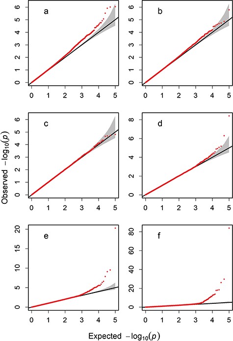
Q–Q plots for six different population sizes for 100 000 simulated SNPs: (a) population size of 50, (b) 100, (c) 200, (d) 500, (e) 1000 and (f) 2000.
Figure 1 showed the six Quantile–Quantile (Q–Q) plots of the genome from the first simulation. The P-values of the statistics used fit well with the expected distribution, and severe inflation was observed for a small number of markers with high P-values. This suggested that population stratification did not occur in the simulated genome, and the type I error rates were well-controlled for the six different population sizes. The approximate and accurate critical threshold values of –log10(p) from the 1st simulation are listed in Table 1 (of statistics in Table S1 of supplementary file). Overall, for Student’s t statistic of the small population and U and chi-squared statistics, all the approximate thresholds fell within the confidence intervals of the permutations. When the population size was less than 200, the approximate thresholds for the t statistics approached the accurate thresholds of the permutations and well-controlled FDRs, while there were considerable differences between the approximate and accurate thresholds for U and chi-squared statistics. For the large population, the approximate thresholds of the U statistics were close to the lower bounds, whereas those of the chi-squared were close to the upper limits of the confidence intervals. In the simulation, the Bonferroni step-down adjustment obtained almost the same thresholds as the Bonferroni correction (6.301 and 7.000 at significance levels of 0.05 and 0.01, respectively), while Benjamini–Hochberg correction underestimated the thresholds compared to the Bonferroni correction. In contrast, the quick approximation gave lower and higher threshold estimates for the t or U and chi-squared or P-value statistics, respectively, than the Bonferroni correction, Bonferroni step-down adjustment and Benjamini–Hochberg correction. The empirical type I error rates generally declined as the critical thresholds increased. As shown in Table 2, the FDRs for the t and U statistics were evaluated to be close to the given significance levels, while the FDRs for the chi-squared and P-value statistics were lower than the given significance levels, which suggested that the quick approximation method often yielded more conservative thresholds for the chi-squared and P-value statistics. Additionally, the U and chi-squared statistics yielded large FDRs for small sample sizes.
The approximate and accurate threshold values of –log10(p) simulated for different population sizes
| n | Statistic | BD | BH | QA | Permutation | Confidence interval | |||||
|---|---|---|---|---|---|---|---|---|---|---|---|
| 0.01 | 0.05 | 0.01 | 0.05 | 0.01 | 0.05 | 0.01 | 0.05 | 0.01 | 0.05 | ||
| 50 | t | 7.044 | 6.312 | 6.915 | 6.243 | (6.835, 7.316) | (6.034, 6.539) | ||||
| U | 6.968 | 6.245 | 9.264 | 8.088 | (9.120, 10.001) | (7.738, 8.597) | |||||
| |${\chi}^2$| | 7.279 | 6.557 | 9.264 | 8.088 | (9.120, 10.001) | (7.738, 8.597) | |||||
| p | 7.000 | 6.301 | 6.997 | 6.288 | 7.316 | 6.538 | 6.915 | 6.243 | (6.835, 7.316) | (6.034, 6.539) | |
| 100 | t | 6.998 | 6.271 | 6.934 | 6.245 | (6.738, 7.004) | (6.067, 6.561) | ||||
| U | 6.963 | 6.239 | 7.969 | 7.063 | (7.709, 8.063) | (6.834, 7.475) | |||||
| |${\chi}^2$| | 7.274 | 6.551 | 7.969 | 7.063 | (7.709, 8.063) | (6.834, 7.475) | |||||
| p | 7.000 | 6.301 | 6.998 | 6.287 | 7.003 | 6.560 | 6.934 | 6.245 | (6.738, 7.004) | (6.067, 6.561) | |
| 200 | t | 6.977 | 6.252 | 6.837 | 6.284 | (6.775, 7.204) | (6.104, 6.487) | ||||
| U | 6.960 | 6.236 | 7.309 | 6.677 | (7.237, 7.733) | (6.472, 6.907) | |||||
| |${\chi}^2$| | 7.271 | 6.548 | 7.309 | 6.677 | (7.237, 7.733) | (6.472, 6.907) | |||||
| p | 7.000 | 6.301 | 6.998 | 6.286 | 7.329 | 6.607 | 6.837 | 6.284 | (6.775, 7.204) | (6.104, 6.487) | |
| 500 | U | 7.247 | 6.245 | 7.521 | 6.372 | (7.265, 7.710) | (6.245, 6.607) | ||||
| |${\chi}^2$| | 7.269 | 6.547 | 7.521 | 6.372 | (7.265, 7.710) | (6.245, 6.607) | |||||
| p | 7.000 | 6.301 | 6.995 | 6.288 | 7.329 | 6.445 | 7.311 | 6.224 | (7.070, 7.489) | (6.102, 6.446) | |
| 1000 | U | 6.958 | 6.323 | 7.046 | 6.468 | (6.874, 7.655) | (6.319, 6.776) | ||||
| |${\chi}^2$| | 7.269 | 6.546 | 7.046 | 6.468 | (6.874, 7.655) | (6.319, 6.776) | |||||
| p | 7.000 | 6.301 | 6.997 | 6.281 | 7.329 | 6.607 | 6.953 | 6.391 | (6.786, 7.544) | (6.245, 6.691) | |
| 2000 | U | 6.958 | 6.234 | 7.066 | 6.403 | (6.925, 7.274) | (6.171, 6.637) | ||||
| |${\chi}^2$| | 7.268 | 6.546 | 7.066 | 6.403 | (6.925, 7.274) | (6.171, 6.637) | |||||
| p | 7.000 | 6.301 | 6.997 | 6.290 | 7.231 | 6.499 | 7.004 | 6.175 | (6.913, 7.232) | (6.042, 6.500) | |
n is population size; BD represents Bonferroni step-down adjustment, BH controlling FDR and QA quick approximation methods.
The simulated false discovery rates generated by different approximate thresholds
| m | n | Distribution | BD | BH | U | t | |${\chi}^2$| | p | ||||||
|---|---|---|---|---|---|---|---|---|---|---|---|---|---|---|
| 0.01 | 0.05 | 0.01 | 0.05 | 0.01 | 0.05 | 0.01 | 0.05 | 0.01 | 0.05 | 0.01 | 0.05 | |||
| 100000 | 50 | N(0,6) | 0.010 | 0.040 | 0.010 | 0.044 | 0.269 | 0.798 | 0.009 | 0.037 | 0.161 | 0.495 | 0.005 | 0.023 |
| 100 | 0.007 | 0.045 | 0.007 | 0.047 | 0.065 | 0.250 | 0.007 | 0.049 | 0.040 | 0.138 | 0.001 | 0.024 | ||
| 200 | 0.008 | 0.048 | 0.008 | 0.049 | 0.033 | 0.134 | 0.008 | 0.050 | 0.013 | 0.068 | 0.003 | 0.020 | ||
| 500 | 0.017 | 0.042 | 0.017 | 0.044 | 0.011 | 0.060 | 0.015 | 0.032 | 0.010 | 0.018 | ||||
| 1000 | 0.009 | 0.067 | 0.009 | 0.069 | 0.013 | 0.059 | 0.009 | 0.042 | 0.006 | 0.030 | ||||
| 2000 | 0.011 | 0.056 | 0.011 | 0.059 | 0.014 | 0.059 | 0.006 | 0.032 | 0.005 | 0.023 | ||||
| 10000 | 100 | 0.008 | 0.059 | 0.008 | 0.062 | 0.046 | 0.196 | 0.001 | 0.051 | 0.027 | 0.104 | 0.005 | 0.031 | |
| 2000 | 0.015 | 0.039 | 0.015 | 0.039 | 0.019 | 0.049 | 0.013 | 0.026 | 0.010 | 0.019 | ||||
| 50000 | 100 | 0.016 | 0.051 | 0.017 | 0.054 | 0.064 | 0.207 | 0.011 | 0.051 | 0.041 | 0.108 | 0.010 | 0.026 | |
| 2000 | 0.010 | 0.055 | 0.010 | 0.061 | 0.014 | 0.052 | 0.005 | 0.035 | 0.004 | 0.028 | ||||
| 500000 | 100 | 0.009 | 0.048 | 0.009 | 0.053 | 0.094 | 0.354 | 0.008 | 0.050 | 0.053 | 0.204 | 0.002 | 0.027 | |
| 2000 | 0.011 | 0.035 | 0.011 | 0.037 | 0.013 | 0.050 | 0.005 | 0.020 | 0.004 | 0.016 | ||||
| 100000 | 100 | U(1.5,10) | 0.014 | 0.050 | 0.014 | 0.054 | 0.064 | 0.272 | 0.014 | 0.052 | 0.040 | 0.152 | 0.006 | 0.031 |
| 2000 | 0.012 | 0.070 | 0.012 | 0.073 | 0.018 | 0.076 | 0.007 | 0.042 | 0.007 | 0.030 | ||||
| 100 | |${\chi}^2$|(3) | 0.093 | 0.258 | 0.100 | 0.325 | 0.330 | 0.325 | 0.093 | 0.273 | 0.222 | 0.561 | 0.060 | 0.164 | |
| 2000 | 0.010 | 0.058 | 0.010 | 0.061 | 0.012 | 0.077 | 0.007 | 0.047 | 0.006 | 0.039 | ||||
n is population size, m is the number of SNPs and BD represents Bonferroni step-down adjustment and BH controlling FDR methods.
Table S2 showed the approximate and accurate threshold estimates of –log10(p) that were obtained with the three competing methods and the permutation test for different numbers of SNPs (Table S3 of statistics in supplementary file). Among the three competing methods, the orders of the approximate threshold estimates did not vary with the simulated numbers of SNPs. For either the t statistics for the small population or the U statistics for the large population, the quick approximation method could generate empirical type I error rates close to the given significance levels. When using the uniform and chi-squared distributions to simulate the phenotypes, the three competing methods could robustly estimate the thresholds and control FDRs for the t statistics for the small population and the U and chi-squared statistics for the large population. For the small population, however, the permutation tests appeared to overestimate the accurate thresholds by the t statistics if the phenotype was generated from the more skewed distribution, such as chi-squared distribution.
Case analyses
We applied the quick approximation method to re-determine the critical thresholds for a GWAS for eight Arabidopsis thaliana (Arabidopsis) traits [25] (available online at http://archive.gramene.org/db/diversity/diversity_view) and four mouse traits [26] (available online at http://gscan.well.ox.ac.uk). In the two datasets, a total of 216 100 SNPs were genotyped for 199 Arabidopsis and 10 100 SNPs for 1940 mice. The Q–Q plots for phenotypes (not shown) showed reasonable non-normality of the X44_FRI, X59_FT.GH and X57_FT.Field traits in Arabidopsis. There were different sample sizes for the analyzed traits, because records were missing for some of the individuals. To eliminate confounding effects from the population structure, as shown in Figures S1 and S2 in the supplementary files, we applied the efficient mixed-model association eXpedited method [27] to the GWAS for these traits. For Arabidopsis traits with less than 200 records, Student’s t statistic was chosen to detect the association of the phenotype with the SNPs, while the U and chi-squared statistics were used for mouse traits from a large population. Phenotypes were shuffled 1000 times for the permutation tests.
Table 3 shows the approximate and accurate thresholds of –log10(p) for eight Arabidopsis traits and four mouse traits (Table S4 of statistics in supplementary file). All approximate thresholds of the t and U statistics for the Arabidopsis and mouse traits, respectively, fell within the confidence intervals of permutation tests, with the exception of the three non-normal Arabidopsis traits. As shown in the simulations, the permutation test indeed overestimated accurate thresholds for non-normal Arabidopsis traits, resulting in accurate threshold estimates that were far greater than those by the Bonferroni correction. For the four mouse traits, the approximate thresholds of chi-squared statistics were very close to the upper limits of confidence intervals, although they were not within the corresponding confidence intervals. For mouse traits, Benjamini–Hochberg correction underestimated the critical thresholds, as compared to the quick approximation and permutation test.
The approximate and accurate threshold values of –log10(p) for eight Arabidopsis traits and four mouse traits
| Traits | n | Statistic | BD | BH | QA | Permutation | Confidence interval | |||||
|---|---|---|---|---|---|---|---|---|---|---|---|---|
| 0.01 | 0.05 | 0.01 | 0.05 | 0.01 | 0.05 | 0.01 | 0.05 | 0.01 | 0.05 | |||
| Ara-1 | 89 | t | 7.335 | 6.636 | 7.335 | 6.636 | 7.256 | 6.567 | 7.213 | 6.346 | (7.046, 7.392) | (6.192, 6.764) |
| Ara-2 | 93 | 7.335 | 6.636 | 7.335 | 6.636 | 7.263 | 6.536 | 7.424 | 6.544 | (7.133, 7.614) | (6.304, 6.886) | |
| Ara-3 | 93 | 7.335 | 6.636 | 7.335 | 6.636 | 7.256 | 6.529 | 6.879 | 6.347 | (6.712, 7.359) | (6.133, 6.533) | |
| Ara-4 | 100 | 7.335 | 6.636 | 7.335 | 6.636 | 7.259 | 6.475 | 7.161 | 6.437 | (6.903, 7.299) | (6.251, 6.750) | |
| Ara-5 | 110 | 7.335 | 6.636 | 7.335 | 6.636 | 7.262 | 6.536 | 7.339 | 6.670 | (7.188, 7.938) | (6.483, 6.939) | |
| Ara-6 | 164 | 7.335 | 6.636 | 6.733 | 5.681 | 7.248 | 6.523 | 7.547 | 6.605 | (7.462, 8.125) | (6.471, 7.100) | |
| Ara-7 | 166 | 7.335 | 6.636 | 7.335 | 5.045 | 7.246 | 6.522 | 7.585 | 6.894 | (7.429, 7.813) | (6.681, 7.204) | |
| Ara-8 | 180 | 7.335 | 6.636 | 5.954 | 5.023 | 7.259 | 6.535 | 8.053 | 7.075 | (7.868, 8.225) | (6.736, 7.691) | |
| Mice-1 | 1405 | U | 6.040 | 5.341 | 4.378 | 3.579 | 5.670 | 4.940 | 5.580 | 4.863 | (5.485, 5.705) | (4.647, 5.184) |
| |${\chi}^2$| | 5.983 | 5.255 | 5.580 | 4.863 | (5.485, 5.705) | (4.647, 5.184) | ||||||
| Mice-2 | 1571 | U | 6.040 | 5.341 | 4.999 | 3.910 | 5.684 | 4.954 | 5.486 | 4.873 | (5.373, 5.828) | (4.662, 5.151) |
| |${\chi}^2$| | 5.997 | 5.269 | 5.486 | 4.873 | (5.373, 5.828) | (4.662, 5.151) | ||||||
| Mice-3 | 1642 | U | 6.041 | 5.342 | 4.962 | 4.228 | 5.675 | 4.945 | 5.509 | 4.902 | (5.375, 5.896) | (4.676, 5.189) |
| |${\chi}^2$| | 5.988 | 5.260 | 5.509 | 4.902 | (5.375, 5.896) | (4.676, 5.189) | ||||||
| Mice-4 | 1643 | U | 6.041 | 5.342 | 5.041 | 4.112 | 5.669 | 4.939 | 5.523 | 4.803 | (5.353, 5.918) | (4.622, 5.048) |
| |${\chi}^2$| | 5.982 | 5.254 | 5.523 | 4.803 | (5.353, 5.918) | (4.622, 5.048) | ||||||
n is population size; BD represents Bonferroni step-down adjustment, BH controlling FDR and QA quick approximation methods. Ara-1–8 represent the trait X182_Hypocotyl.length, X278_Germ.in.dark, X29_Se82, X272_Seedling.Growth, X283_Storage.56.days, X44_FRI, X59_FT.GH, X57_FT.Field, respectively, in Arabidopsis. Mice-1–4 refer to the trait Imm.PctCD8, Haem.MCH, FPS.Pre.Bang.ToneMean, FPS.Pre.Bang.Mean, respectively, in mouse.
The critical thresholds by Bonferroni correction were 7.335 and 6.636 at the significance levels of 1% and 5% for Arabidopsis traits and 6.041 and 5.342 for mouse traits, which were almost the same by both Bonferroni step-down adjustment and Benjamini–Hochberg correction. In Figures 2 and S3, we depicted the Manhattan plots for the eight Arabidopsis traits and four mouse traits with horizontal reference lines of the critical thresholds at the significance level of 5% obtained by quick approximation, permutation test and Bonferroni correction. For the traits with the detectable QTNs, such as the four mouse traits and three non-normal Arabidopsis traits, the critical thresholds estimated by quick approximation resided between those by permutation test and Bonferroni correction. Therefore, the number of the QTNs detected by the approximate thresholds was not greater than the accurate thresholds but not less than Bonferroni correction’s thresholds (data not shown).
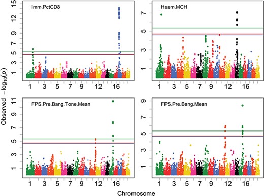
Manhattan plots for the four mouse traits. The red, blue and green horizontal reference lines represent the critical thresholds at the significance level of 5% obtained by quick approximation, permutation test and Bonferroni correction, respectively.
Discussion
Hypothesis testing when a nuisance parameter is present only under the alternative, based on the work of Davies (1977, 1987), has been successfully applied to the quick approximation of critical thresholds for linkage analyses [17, 28, 29]. However, the approximation was evaluated using U and chi-squared statistical values, obtained from a large sample population, without considering the effects of the approximation on the small sample sizes that are often used in a linkage analysis. In fact, a small sample size is often encountered in practice for both linkage analysis and GWASs, such that Student’s t and F statistics were introduced to statistically infer the association of the genetic markers with the traits of interest. Fortunately, for a linear model with unknown residual variances, Davies [30] extended the quick approximation of critical thresholds for the U and chi-squared statistics to the t and F statistics. In this study, we adapted Davies’s results [30–32] for the quick approximation of empirical thresholds in order to apply them to the small and large sample sizes for GWASs. The quick approximation of critical thresholds was developed, according to Fisher’s argument of distributions for P-values, for situations when only the statistical probability P-values for the SNPs are available, regardless of the test statistics. This made the quick approximation of critical thresholds universally applicable for GWASs.
The Bonferroni adjustment was computationally the simplest among the most widely used multiple testing approaches, although it was too conservative and its workload was not associated with a GWAS computation. In contrast, the permutation test, quick approximation, Bonferroni step-down adjustment and Benjamini–Hochberg correction were evaluated by statistical values that were obtained from a GWAS. Given statistical values, the quick approximation took little to no computational time, similar to the Bonferroni step-down adjustment and Benjamini–Hochberg correction, such that their workloads depended almost completely on the GWAS computation. However, the permutation test required a large number of GWAS computations to attain accurate thresholds, and its workload increased drastically as the type I error rate was reduced. The method proposed here for computing approximate thresholds is fast and easy to implement into existing packages for GWASs with minimal effort. The simulations showed that the approximate thresholds fell within the confidence intervals of the accurate thresholds that were calculated by the permutation tests. For the t or U statistics, the quick approximation method performed slightly conservative, as compared to the Bonferroni adjustment, Bonferroni step-down adjustment and Benjamini–Hochberg correction. Additionally, the quick approximation was relatively robust for non-normality but should be used with caution if there is a remarkable departure from normality, especially for small populations. The case analysis demonstrated that the quick method yields thresholds similar to those obtained by the permutation test.
Standard normal statistics and Student’s t or F statistics, in addition to chi-squared statistics, were used to map QTNs for small and large sample sizes in GWASs.
Hypothesis testing when a nuisance parameter is present only under the alternative was introduced to quickly approximate the critical thresholds for GWASs.
When only the P-values were available, the approximate critical thresholds were estimated with chi-squared statistics, formulated by P-values.
High similarities in the critical thresholds between the accurate and approximate estimations were highlighted by extensive simulations and real data analysis.
Funding
Special Scientific Research Funds for Central Non-profit Institutes, Chinese Academy of Fishery Sciences (2017A001).
Zhiyu Hao is currently a Master’s student in the College of Animal Science and Technology at the Northeast Agricultural University.
Li Jiang is an associate professor in the Research Centre for Aquatic Biotechnology at the Chinese Academy of Fishery Sciences. She is interested in developing and applying statistical methodologies for genome-wide association studies.
Jin Gao is currently a PhD student in the Research Centre for Aquatic Biotechnology at the Chinese Academy of Fishery Sciences.
Jinhua Ye is a lecturer in the Department of Mathematics at the Heilongjiang Bayi Agricultural University. Her research interest is in mapping quantitative trait loci by genome-wide association studies.
Jingli Zhao is currently a Master’s student in the Research Centre for Aquatic Biotechnology at the Chinese Academy of Fishery Sciences.
Shuling Li is a professor in the College of Life Science at the Northeast Agricultural University. Her research focuses on animal behavior genetics and genomics.
Runqing Yang is a professor in the Research Centre for Aquatic Biotechnology at the Chinese Academy of Fishery Sciences. He is interested in developing statistical methodologies for genome-wide association studies.
