


Abstract
Principal components (PCs) are widely used in statistics and refer to a relatively small number of uncorrelated variables derived from an initial pool of variables, while explaining as much of the total variance as possible. Also in statistical genetics, principal component analysis (PCA) is a popular technique. To achieve optimal results, a thorough understanding about the different implementations of PCA is required and their impact on study results, compared to alternative approaches. In this review, we focus on the possibilities, limitations and role of PCs in ancestry prediction, genome-wide association studies, rare variants analyses, imputation strategies, meta-analysis and epistasis detection. We also describe several variations of classic PCA that deserve increased attention in statistical genetics applications.
Introduction
Principal component analysis (PCA) is one of the oldest multivariate techniques in statistics, having its roots in the 19th century with scientists such as Cauchy and Pearson [1]. The term principal component (PC) itself originates from the work of Hotelling in his seminal 20th century work on the ‘analysis of a complex of statistical variables into principal components’ [2]. About five decades later, PCA found its way into regression analysis to summarize large numbers of possibly correlated variables into a representative reduced set of uncorrelated variables (PCs), and as a valuable tool for dimensionality reduction or large data visualization [3–5]. With the emergence of high-density micro-arrays for gene expression [6] and the rise of sequencing initiatives in model organisms [7] and humans [8], ‘large data’ rapidly turned into ‘big data’, and condensing data for visualization or analysis purposes became a necessity. In genetics, by exploiting DNA-based genetic variants, PCA has shown its usefulness to infer shared genetic ancestry from unrelated samples [9–12] and from related samples [13], as covariates to correct for confounding due to population structure in genome-wide association and interaction studies [10, 14] to study and understand human population migrations [15], to reduce the huge genetic variant dimensionality for cluster analysis in clustering of subpopulations [16], to impute missing genetic variants [17] and to detect outliers for population stratification (PS) in genome-wide association studies [18].
This review is organized in four main parts. In the first two parts (Classical PCA and Contextual PCA), we give an overview of different approaches to compute PCs. Better understanding of the data-dependencies and variable selection procedures involved in PCA is important to understand the challenges in validating or replicating PC-involved analyses. Special attention is given to data standardization, pre- and post-analysis considerations. Confounding by population structure is taken as leading example. In the third part (Variations to Classical PCA), we review generalizations to classic PCA, including robust and sparse PCA, and generalized and kernel PCA. In the fourth part (Remaining Challenges), we elaborate on remaining challenges for PCA exploitation in statistical genetics to accommodate specific study designs or input data characteristics.
Classic PCA
Different computational viewpoints
Broadly speaking there are two commonly used approaches of PCA that give rise to the same result [19]. In the first approach, PCs are defined by finding a small number of linear combinations of the variables that account for most of the variance in the observed data [2]. In the second approach, PCA can be defined by finding the orthogonal linear projections that minimize the mean squared distance between the original data points and their projections [20].
In particular, the main idea of the linear PCA is to describe the variation in a set of |$M$| correlated variables, |$X=\left({X}_1,\dots, {X}_M\right)$|, in terms of a new set of uncorrelated linear combinations called PCs, |$Z=\left({Z}_1,\dots, {Z}_M\right)$| given as |$Z= VX$|, with the |$j$|th PC given by |${Z}_j={V}_{j1}{X}_1+\cdots +{V}_{jM}{X}_M$|, and |$V$|’s representing coefficients or weights in the linear combination. Often it is possible to retain most of the variability with much fewer variables than |$M$|. In particular, the first few PCs will account for a substantial proportion of the variation in the original variables, |$X$|, and can, consequently, be used to provide a convenient lower-dimensional summary of these variables. The coefficients V are commonly obtained via matrix factorization such as singular value decomposition (SVD) or eigenvalue decomposition (EVD).
SVD
The columns of |$Z$| are the PCs, and the columns of |$V$| are the corresponding unit-scale loadings of the PCs. Moreover, the PCs can be computed multiplying |$U$| (left singular matrix) with |$\Lambda$| (the matrix of singular values). We note that when the rank R of |$X\ \mathrm{equals}\ M$|, we can compute all |$M$| PCs. In contrast, if |$R<M$|, the number of PCs to be computed is less than the number of variables. Usually the first |$P\ \mathrm{PCs},P\ll \min \left(N,M\right),$| are chosen to represent the data. In summary, the adoption of SVD in PCA is a computationally efficient method for finding orthogonal PCs, thus achieving a minimal squared loss of information [21].
EVD
Comparing equations ( 2) and (3) we have |$D={\varLambda}^2.$| Also, using equation (1) and (2), |${Z}^TZ$| = D, implying that there is a direct relationship between the variance of PCs and the eigenvalues of |${X}^TX$| or singular values of |$X$|.
PC computation in high-dimensional genetics data
where the columns of |$U$| are eigenvectors, and |$D$| is a diagonal matrix of positive eigenvalues of |$X{X}^T$|. Compared to the previous formula ( 3), here the roles of variables and samples are swapped [22]. Similarly, compared to SVD, we have |$D={\varLambda}^2$|, meaning that the singular values of |$X$| are equal to the square roots of the eigenvalues of |$X{X}^T$|, |$\varLambda ={D}^{1/2}$| and the columns of |$U$| are the left singular vectors of |$X$| or the eigenvectors of |$X{X}^T$|. The rescaled eigenvectors of |${X}^T$|, |$U{D}^{1/2}$| can be used as principal coordinates of the subjects. One can also compute the loadings, |${V}^T={D}^{-1/2}{U}^TX$| and then the PCs are |$Z=X{\left({V}^T\right)}^T$|.
In practice, the exploitation of PCs requires making choices about the actual data matrix to be used, implying carefully thinking about variable selection, sample selection and a priori data transformations. Once PCs are obtained, the main challenges are to decide upon the most informative PCs (which may be context dependent) and to interpret them. In the next section, we discuss these aspects in more detail, taking population structure in statistical genetics as leading context.
Contextual PCA
PS as a confounder in genetic association studies
In the context of genetic association studies (GWAS), PS refers to confounding of the association by the presence of genetically distinct subgroupings. Specifically, PS occurs if (1) the genetic risk of disease depends on the ethnic background of the individual, (2) the genetic variants under investigation are differently frequent in different ethnic subgroups and (3) cases and controls in the study are heterogeneous with regard to the ethnic background [23, 24]. The use of PCA to explicitly model PS is one of the most popular strategies to remove the confounding effect of PS in GWAS. Alternatively, family-based case–control designs offer protection from PS but at the expense of some loss of practicality and power from overmatching on genotype [25]. Several causes exist for PS, the basic one being genetic ancestry as a result of non-random mating between subgroups in a population due to various reasons (social, cultural, geographical). Confounding, cryptic relatedness (i.e. unobserved ancestral relationships between individual cases and controls who are naively treated as independent in association testing) and selection bias are potential consequences of PS [25].
Handling PS
Propensity scores
In general, confounding can be addressed by the so-called propensity scores that were initially developed by Rosenbaum and Rubin [26], and widely known in classic epidemiology. The concept was adapted to the confounding of genetic associations by PS in [27, 28].
Structured Association and Genomic Control
Structured Association (SA) [29], Genomic Control (GC) [30], PCA-based methods and mixed models currently belong to the most popular approaches to handle confounding in GWAS. SA and GC have gone through several modifications, since their conception. For a historical perspective on SA and GC methods, we refer to the Supplementary Material.
PCA
In contrast to SA and GC methods, in PCA the data are transformed to a new coordinate system such that the projection of the data along the first new coordinate has the largest variance; the second PC has the second largest variance, and so on. The availability of genome-wide Single Nucleotide Polymorphism (SNP) panels, the relative straightforwardness of PCA, its ease of use, the availability of efficient algorithms [31] and its ability to detect individuals with unusual or differential ancestry (Patterson et al. [32], Paschou et al. [33], Heath et al. [34], Reich et al. [15], Novembre et al. [9]) has increased the popularity of using PCs in the context of GWAS that are possibly hampered by PS issues (e.g. Himes et al. [35], Tantisira et al. [36]).
A popular PCA-based method was introduced by Price et al. [10]. Their method EIGENSOFT/EIGENSTRAT consists of three steps. First, applying PCA to genotype data to infer continuous axes of genetic variation and taking the top eigenvectors of a covariance matrix between samples. The top PCs are viewed as continuous axes of variation that reflect subpopulation genetic variation in the sample. That is, individuals with similar values for a particular top PC will have similar ancestry for that axis. Second, adjusting genotypes and phenotypes by amounts attributable to ancestry along each axis, via computing residuals of linear regressions of PCs on trait and PCs on each genotype. Third, computing association statistics using ancestry-adjusted genotypes and phenotypes. Their method is implemented in the software EIGENSTRAT. For a better understanding of the working mechanisms of EIGENSTRAT, see also Ma and Amos [37].
Engelhardt and Stephens [38] showed that admixture-based models such as those provided by STRUCTURE and PCA can be viewed within a single unifying framework of matrix factorization. The main advantage of a PCA-based approach is that it avoids the need to actually infer the population structure from the available data. However, although this method was shown to outperform GC and is much simpler and computationally faster than SA, it does suffer from some drawbacks that are related to the use of PCs as corrective factors.
In their paper, Popescu et al. [39] proposed PSIKO a linear-kernel PCA-based approach that returns significant PCs of a dataset similar to EIGENSTRAT [10] with the additional feature of generating Q-matrices comparable to those produced by STRUCTURE, ADMIXTURE and sparse nonnegative matrix factorization. In addition, PISKO has the advantage of being scalable for large datasets. Similarly, Ma and Amos [37] considered the calculation of theoretical or ‘population’ PCs from the estimates of the variance–covariance parameters that can be used in GWAS to control the confounding effect of population structure in a regression setting. They showed that their method is equivalent to adjusting population structure by subtracting the population mean from the allele counts and demonstrated that it works better than or as well as EIGENSTRAT [10].
PCs as fixed effects in linear models
where |$Y$| is a vector of phenotype values, |$\mu$| is the scalar mean term, |${X}_j$| is the jth SNP with scalar regression coefficient |$\beta$|, |$W=\left({Z}_{(1)},\cdots, {Z}_{(c)}\right)$| are the first |$c$| PCs from |$Z$|, |$\theta =\left({\theta}_1,\dots, {\theta}_c\right)$| is the corresponding coefficient vector and |$e$| is a normally distributed residual error term with variance |${\sigma}_e^2$|. In this regression setting, the PCs are treated as fixed effects, such that direct maximization of the likelihood provides estimates of all parameters. However, determining the relevant number of PCs to be included in the regression model that efficiently captures population structure needs special attention. More general, depending on the type of response variable one can choose the relevant model from generalized linear models (GLMs). Figure 1 illustrates the GWAS results on Crohn’s disease [40] without correcting for population structure and with correction for structure using the top five PCs. Fewer significant SNPs are obtained with correction for structure (above the horizontal GWAS significance line) compared to the analysis without correction for structure.
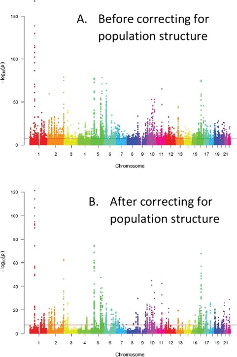
Correcting for structure with PCA in GWAS–Manhattan plots. Before correcting for structure too many significant SNPs found that could be false positives (above the horizontal line or the genome wide significance level) compared to after population structure correction. A. Before correcting for population structure, B. After correcting for population structure.
Table 1 presents the significant SNPs resulting from using GC and PCA methods after adjusting for multiple testing using genome-wide correction. The GC inflation factor |$\left({\lambda}_{obs}=8.764\right)$| or the adjusting GC for large samples |$\left({\lambda}_{1000}=1.327\right)$| (see supplementary material) suggests the existence of strong population structure.
Number of significantly associated SNPs with Crohn’s disease resulting based on GC and PCA methods
| Methods | GC Inflation Factor (|$\boldsymbol{\lambda}$|) | Genome-wide Correction (|$\boldsymbol{P}<\mathbf{5}\times {\mathbf{10}}^{-\mathbf{8}}$|) |
|---|---|---|
| Without Population Correction | ____ | 3266 |
| GC | 8.764 | 31 |
| GC with large sample correction | 1.327 | 2034 |
| PCA | 1.048 | 961 |
Without correcting for population structure, the number of significant SNPs is highly inflated (3266 SNPs) even after correcting for multiple testing. The use of the GC method with the observed GC factor |$\left({\lambda}_{obs}=8.764\right)$| is too conservative and provides too few significantly associated SNPs, whereas the GC method with the adjusted factor |$\left({\lambda}_{1000}=1.327\right)$| reduces the inflated number of significant SNPs by about one-third (2034 SNPs). However, there will be still an increased number of false positives because the inflation factor is greater than 1.0, and the confounding population structure is not adequately controlled using GC. On the other hand, using PCA with the top five PCs further reduced the number of significantly related SNPs to 961. After performing PCA, the computed inflation factor reduces to 1.048, which is very close to 1.0, suggesting that no strong population structure remains to increase the false positives. Thus, for this dataset PCA performs far better than GC in controlling population structure.
PCs to express random effects
With the recent development of computationally efficient algorithms, linear mixed models (LMMs) have become popular in GWAS for controlling PS as well as familial or cryptic relatedness [41]. The LMM is defined as
|$Y=\mu +{\beta}_j{X}_j+b+\varepsilon$|, |$b\sim N\left(0,{\sigma}_g^2K\right)$|, and |$\varepsilon \sim N\left(0,{\sigma}_e^2\right)$|,
where |$b$| is a random effect vector of dimension |$N$| with a multivariate Gaussian distribution reflecting polygenic background, |${\sigma}_g^2$| is the additive genetic variance and |$K$| is the genetic similarity matrix of dimension |$N\times N$| between all pairs of individuals so that |${K}_{jl}$| represents the similarity between individuals |$j$| and |$l$|.
Several methods for the estimation of a kinship or genetic similarity matrix from a large number of markers have been introduced [42] that include using an identical-by-descent (IBD) matrix, an identical-by-state (IBS) allele-sharing matrix, a maximum-likelihood kinship matrix [43] or a Monte Carlo simulation-based matrix [44]. Comparisons of different kinship matrices for explaining genetic differentiation among populations show similar results with small quantitative differences [45]. However, studies on the association mapping of Arabidopsis thaliana in a structured population show that a simple IBS allele-sharing matrix effectively corrects for confounding from population structure, even better than more sophisticated methods [46]. The simple IBS allele-sharing matrix approach is implemented in the Efficient Mixed-Model Association (EMMA) and Genome-Wide Efficient Mixed-Model Association (GEMMA) software packages for the analysis of mixed models [88, 96].
In the mixed model setting, population structure is treated using a random effect without explicitly stating it in terms of PCs. Fitting the model involves integrating over the random effect vector |$b$| with respect to the Gaussian distribution so that the likelihood is maximized with respect to the parameters |$\left\{\beta, \mu, {\sigma}_g^2,{\sigma}_e^2\right\}$|. Various software solutions for fitting LMM are available such as EMMA [42], EMMA eXpedited [47], GEMMA [48], Factored Spectrally Transformed LMM [49] and GeneABEL [50].
where |$Z$| is a matrix of all PC scores.
Comparing equations (4) and (5), Hoffman [51] observed that modelling PCs as fixed and expressing random effects in terms of PCs in LMMs share the same underlying regression model but the LLM includes all PCs and the fixed effects model only the first |$c$| selected PCs.
Further, Hoffman [51] noted that including PCs that are not biologically relevant to the given phenotype can dilute the influence of relevant PCs and degrade the quality of the correction since the random effect is governed by a single global parameter. As a solution Hoffman [51] introduced a novel data-adaptive low rank LMM to learn the dimensionality of the correction for population structure and kinship effective degrees of freedom (a metric of model complexity). This approach integrates the test of association using LMM and the selection of a subset of PCs to correct for genetic confounding. Similarly, Listgarten et al. [52] proposed the FaST-LMM-Set method, which is a LMM where a genetic relationship matrix is constructed from a subset of top associated SNPs that are more likely to be causal. However, Yang et al. [53] showed that limiting the genetic relationship matrix to a subset of SNPs can result in insufficient correction for PS, leading to significantly inflated statistics and false positive associations. In remedy to this problem, Tucker et al. [54] proposed PC-Select, a novel hybrid approach that includes the PCs of the genotype matrix as fixed effects in FaSTLMM Select method of Listgarten et al. [52].
PS as a confounder to patient subtyping
The problem of structure detection in patients or populations is largely a clustering problem. Clustering methods have been around for quite some time and have been applied to a variety of fields (for a brief review, see for instance Kotsiantis and Pintelas [55]). However, the integration of more sophisticated clustering methods in genetics is fairly new and constantly evolving (e.g. Lee et al. [56], Lawson and Falush [16]). Lawson and Falush [16] have reviewed a range of common clustering algorithms and evaluated their performance through a simulation study. In the clustering step they computed generic methods such as MCLUST, K-means and UPGMA, based on the genetic similarity matrix first using a PCA as dimension-reduction technique. The latter approach with PCA has led to a substantial improvement on the performance of most of these clustering methods referred to as spectral MCLUST, spectral K-means and spectral UPGMA. Solovieff et al. [57] developed a novel algorithm based on PCs to cluster individuals into groups with similar ancestral backgrounds. They demonstrated the effectiveness of their algorithm in real and simulated data and showed that matching cases and controls using the clusters assigned by the algorithm substantially reduce PS bias. Similarly, PCs have been used to derive stable clusterings [58].
Recently, the application of PCA to control the confounding effect of population structure on molecular classification of Crohn’s Disease was considered in [59]. Maus et al. [59] used cluster analysis on ancestry-informative genetic markers to identify genetic-based subgroups of Crohn’s disease while taking into account possible confounding by population structure. The authors demonstrated that without correction for PS clusters seems to be influenced by PS while with correction for PS, clusters of Crohn’s disease subtypes are unrelated to continental origin of individuals.
PCA pre-analysis considerations
Data transformation
PCA is not a scale invariant method, namely the extracted PCs are dependent on the units of measurement of the original variables and the range of values they assume [60]. If in addition each element of X is divided by |$\sqrt{N}$| or |$\sqrt{N-1}$|, then the |$M\times M$| matrix |${X}^TX$| represents a covariance matrix, and PCA may be referred to as covariance PCA. To deal with different measurement units of variables, matrix columns in X may be standardized, by dividing each variable value by the square root of the sum of all the squared elements of this variable (i.e. unit norm). In this scenario, |${X}^TX$| represents a correlation matrix, and PCA may be referred to as correlation PCA. There is no straightforward relationship between the PCs obtained from a correlation matrix and those based on the corresponding covariance matrix. Which one to use has been a topic of discussion in the literature; see, for example, [21, 61]. Jolliffe [21] gave an example to illustrate the dangers in using a covariance matrix to find PCs when the variables have widely differing variances: the first few PCs will usually contain little information apart from the relative sizes of variances, information that is available without a PCA. On the other hand, correlation matrix PCs have the particular disadvantage that it is difficult to base statistical inference regarding PCs on correlation matrices because they give coefficients for standardized variables and are therefore not easy to interpret directly. Still, in case that the unit of measurements differs substantially or that there are large differences between the variances of the original variables, it is suggested to use the correlation matrix instead of the covariance matrix.
For genetic data that comprised of SNPs to compute PCs, the correlation-based data standardization approach in Price et al. [10] and Patterson et al. [32] goes as follows. Let |$G=\left({g}_{ij}\right)$| be a matrix of genotypes for individual |$i$| and SNP |$j$|, where |$i=1,\dots, N$|, |$j=1,\dots, M$| and |${g}_{ij}$| takes a value from |$\left\{0,1,2\right\}$| that represents the number of copies of the minor allele that individual |$i$| has at SNP |$j$|. Consider SNP |$j$|, the |$j$|th column of |$G$|. Let |${\mu}_j=\frac{1}{N}{\sum}_i{g}_{ij}$| be the mean and |${\sigma}_j=\sqrt{p_j\left(1-{p}_j\right)}$| be an estimate of the SD of SNP |$j$|, where |${p}_j$| defined as |${p}_j={\mu}_j/2$| is an estimate of the underlying allele frequency of SNP |$j$| (Patterson et al. [32], or |${p}_j=\left(1+{\sum}_i{g}_{ij}\right)/\left(2+2N\right)$| is a posterior estimate of the unobserved underlying allele frequency of SNP |$j$| [10]). The standardized genotype score for individual |$i$| and SNP |$j$| is given by |${X}_{ij}=\frac{g_{ij}-{\mu}_j}{\sigma_j}$| , and we denote the standardized data matrix of dimension |$N\times M$| by |$\boldsymbol{X}$| that can be used for PCA. Alternatively, Niu et al. [14] used only mean subtracted standardization for PCA computation from genotypes data, which is equivalent to working with the covariance matrix to correct the effect of population structure on epistasis investigation.
Variable (SNPs or other markers) selection
In classical multivariate analysis, the presence of highly correlated variables often complicates the data analysis without giving any extra information. For example, if two variables are highly correlated, one of the variables may be discarded with little loss of information as the two variables seem to be redundant. In PCA many methods have been discussed on how to discard redundant variables (see for example, [62]). These methods depend on multiple correlation coefficients, PCs or cluster analysis. In the GWAS literature it is a common practice as a data quality step to prune groups of SNPs with high linkage disequilibrium (LD) or regions with LD extending over long genome distances (long-range LD) or other artefacts such as inversions prior to performing PCA [63–66].
In their review of key concepts underlying GWAS, Bush and Moore [67] described LD as a property of SNPs on a contiguous stretch of genomic sequence that describes the degree to which an allele of one SNP is inherited or correlated with an allele of another SNP within a population. LD is generally reported in terms of |${r}^2$|, the square of Pearson’s coefficient of correlation. LD patterns in GWAS datasets can distort PCA-based population structure control, showing 'subpopulations' that reflect localized LD phenomena rather than plausible population structure [68]. We and others have shown that it is often necessary to prune SNPs based on LD and other criteria prior to performing PCA to avoid generating eigenvectors that are biased by small clusters of SNPs at specific locations.
LD can confound PCA’s ability to separate disparate populations as in general highly correlated variables may distort the construction of eigenvectors. The question remains which levels of correlatedness are sufficient to bias the association results. Galinsky et al. [66] examined three methods to deal with LD: LD pruning, LD shrinkage and LD regression.
To produce a dataset pruned for LD above a threshold T, one SNP of any pair of SNPs in LD |$ ( r^{2} > T)$| is removed from the data. In practice, |$T=0.20$| is commonly used that guarantees a set of nearly independent SNPs to construct undistorted PCs. LD pruning is implemented in software programs such as PLINK, PriorityPruner and SNPRelate.
LD shrinkage is a more sophisticated method of correcting for LD proposed by Zou et al. [68]. In LD shrinkage, each SNP is weighted by its LD to surrounding SNPs before inclusion in the genetic relationship matrix. For SNP, s, the weight in Zou et al. [68] is given by
$$ {w}_s=\frac{1}{\sqrt{1+\sum_{t\,\in\,window(s)}{r}_{st}^2\ I\left[{r}_{st}^2>T\right]}} $$where |$t\in window(s)$| refers to SNPs that are within some region of the genome surrounding SNP s, |${r}_{st}^2$| is the square of Pearson’s correlation between SNPs |$s$| and |$t$| and |$T$| is a threshold to minimize the effect of noise in the use of |${r}^2$|.
LD regression was originally proposed in [32] and utilized extensively in [69]. The LD regression approach is to transform each SNP into an ‘LD residual’ by fitting a linear regression of each SNP on a small number of adjacent SNPs potentially in LD and taking the residuals from the regression model in the construction of the genetic relationship or similarity matrix.
In their assessment of these methods, in case of datasets that have pervasive LD and large numbers of rare variants, Galinsky et al. [66] showed that using more sophisticated methods has no relevant advantage over the simpler LD pruning approach. In contrast, Zou et al. [68] showed that the LD shrinkage-based PCA method, which is easier to implement than the LD regression approach, effectively removes the artifactual effect of LD patterns, and successfully recovers underlying population structure that is not apparent from classical PCA with LD pruning. In an extensive simulation study, they demonstrated that LD patterns in genome-wide association datasets can distort PCA-based techniques for stratification control. In fact, if an entire region (e.g. HLA region) is driving a PC, then that can lead to a power loss to detect an association between any of the markers in that region and the trait. In such cases, any of these methods effectively removes the artifactual effect of LD patterns and successfully recovers underlying population structure to adequately control type I error rate and increase the power to detect the causal SNPs [66, 68].
Sample selection
In case/control studies, doing PCA on cases and controls combined or on controls only depends on the assumptions we have about the data. If we assume that the correlation structure itself differs between cases and controls, then it makes sense to do the PCA on controls and then project its results on cases as discussed in [70]. However, if we assume that the structure itself may be the same, but just the factor values are different, then we could use the entire group for the PCA to have a larger sample size and obtain more stable results. The computation of PCs also depends on the sample size ratio between cases and controls, see our simulation results in Figure 1 below. According to [71], PC scores for cases can be obtained based on first extracting PCs from controls and then projecting to cases. This can be done as follows. Partition the genotype data matrix into two |$X={\left[{X}_0,{X}_1\right]}^T$|, where |${X}_0$| is the |${N}_0\ \times \ M$| matrix for controls, and |${X}_1$| is |${N}_1\times M$| matrix for cases. For the controls, compute the eigendecomposition, |${X}_0{X}_0^T={U}_0{D}_0{U}_0^T,$| and select the first |$P$| columns of |${U}_0$| denoted by |${\tilde{U}}_0$|, which has |$N\times P$| dimension. Similarly, select the first |$P$| diagonal elements of |${D}_0$| and denote by |${ \tilde{D}}_0$|. Then calculate the loadings, |${{\tilde{V}}_0}^{\,\,T}={{\tilde{D}}_0}^{-1/2}{\tilde{U}}_0^{T}\,{X}_0$|. The |$P$| PC scores matrix for the entire data is calculated and given by |$Z={\left[{Z}_0,{Z}_1\right]}^T$| where |${Z}_0={X}_0{\left({{\tilde{V}}_0}^{T}\right)}^T$|are PCs for the control subjects and |${Z}_1={X}_1{\left({{\tilde{V}}_0}^T\right)}^T$| are the projected PCs for the case subjects based on loadings calculated from the control data. This approach is used to construct PCs for controlling population structure in fine-mapping inflammatory bowel disease loci to single-variant resolution [40]. Jostins et al. [72] also mentioned this approach in a GWAS context. Of note, this approach requires that the same SNP panel is available for cases and controls. If not, extra steps (e.g. imputation) need to be taken. Alternatively, cases and controls are pooled, prior to PC computation.
To visualize the effect of computing PCs based on the projection and the pooled approach in relation to capturing population structure, we simulate two populations having 500 individuals each with varying case–control ratios (50:50, 60:40 and 80:20). Genotype data from 1000 random SNPs is generated using the Balding–Nichols model [10, 73, 74], assuming Hardy–Weinberg equilibrium (HWE) at each SNP within the two populations. For each SNP, the ancestral allele frequency |${p}_a$| is drawn from a uniform (0.05, 0.95) distribution, and the allele frequency in each population is generated independently from the beta distribution with two parameters |${p}_a\left(1-{F}_{ST}\right)\!/{F}_{ST}\ \mathrm{and}\ \left(1-{p}_a\right)\left(1-{F}_{ST}\right)\!/{F}_{ST}$|, where |${F}_{ST}$| is Wright’s fixation index, a measure of genetic divergence among subpopulations [75], which is set at 0.01.
The first two PC scores are computed from the simulation data based on the pooled (overall case/control) data and using the projection approach first by computing PCs from the controls and then using the loadings to project PC scores for the cases as described above. The PC plots are displayed in Figure 2 that shows a clear separation between the two populations. Figure 2a shows the PC plot of the pooled data that is similar for all case–control scenarios. Whereas the PC plots of the projected approach are shown in Figure 2b, c and d. Here the projected PC scores for cases (red and blue for population 1 and 2, respectively) tend to concentrate around the two centroids. With increasing discrepancies in the ratio of cases to controls the projected PC plots of cases are shifted away from their corresponding control plots and formed artificial grouping. Our large sample size (1000 or more) simulation results (not reported here) showed that there is no relevant impact of PC computation based on the pooled or the projected approach on epistasis studies with adjusting for population structure.
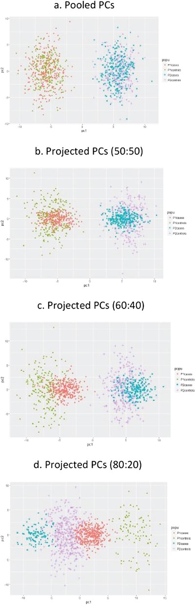
Linear PCA on balanced and imbalanced case–control data—indicating that this may have repercussions depending on the context for which PCs are used. a. Pooled Pcs, b. Projected Pcs (50:50), c. Projected Pcs (60:40), d. Projected Pcs (80:20).
PCA post-analysis considerations
Determining the most informative PCs
There are many approaches that have been proposed and evaluated in the multivariate literature to estimate the relevant number of PCs. Jolliffe [21] reviewed the most frequently used PC selection approaches and grouped the methods into three categories: ad hoc methods that are intuitively plausible and work quite well in practice, methods including formal statistical tests that make distributional assumptions and methods that use computationally intensive procedures such as permutation, cross-validation, bootstrap or jackknife that do not require distributional assumptions. Ad hoc methods include the scree plot [76], Kaiser’s eigenvalue greater than one [77] and Velicer’s minimum average partial correlations [78]. The scree plot is a useful visual aid for determining an appropriate number of PCs. It is based on the plot of eigenvalues against the component numbers. To determine the appropriate number of PCs, one has to look for an ‘elbow or inflection point’ in the scree plot.
Formal test-based methods include, for example, the Tracy–Widom test. Permutation-based methods include various functions defined on the eigenvalues (see Jolliffe [21]) and the permutation tests proposed by Dray [79] based on measurements of similarity between matrices. Interestingly more sophisticated methods to select the number of PCs include those based on the estimated ‘generalized error’ [80], in analogy with optimization of feed-forward artificial networks, or distance-based regression [81], but are seldom used in omics data analysis applications.
In the context of confounder correction in GWAS, the retained number of PCs commonly varies between 1 and 10. Typically 5 or 10 PCs are in wide use but 1 or 2 PCs are also used occasionally. One way to determine the most relevant PCs to capture confounding in GWAs due to shared genetic ancestry is based on a trial-and-error approach where the analysis is repeated for different selections of PCs. In contrast, Patterson et al. [32] proposed using the Tracy–Widom statistic to assess significance of eigenvalues to select PCs. However, this testing procedure tends to identify a large number of significant PCs, a problem which may in part be resolved by the procedure proposed by Lee et al. [82] using a permutation approach. Apart from the approaches described before, the specific context of GWAS has given rise to additional strategies. We refer to Peloso and Lunetta [83] who gave a brief summary of some of the PC selection methods to adjust for population structure in GWAS, including reduction in inflation of GC lambda [84], PC-Finder that is a permutation-based test using a pseudo F-statistic [81], PCs significantly related to the outcome [85] and PCs significant according to the Tracy–Widom statistic and cluster membership as covariates [86].
Notably, for PCs to act as confounding variables in a genome-wide association regression model, they should be associated to both the genetic marker and trait under study. For that reason, the optimal number of PCs can be determined based on a forward or stepwise regression model. Hence, another way to determine the optimal number of PCs is to fix the genetic marker of interest but to allow an automated variable selection method to choose the number of required PCs. In particular, such an approach involves starting with no covariates at all, testing the addition of each computed PC using a chosen model comparison criterion and adding the PC that provides the best model improvement. This scenario is repeated until no other PC covariate can improve the model. The drawback is that too little of the trait variation may be left to get explained by genetic markers. Also, a priori inclusion of the genetic marker of interest (to be tested for association with the trait) in the null model is not recommended to avoid multicollinearity problems caused by strong SNP-PC associations. In this regard, [85] included PCs associated with case status as covariates for population structure correction in an association model and found that the reduction in the genomic inflation factor was similar for PCs computed for subsets of genome-wide SNPs with varying levels of LD. However, they noticed that for some SNP subsets, the PCs associated with case status and used in the structure adjustment heavily weighted small numbers of SNPs, which could lead to reduced power to detect true associations in those genomic regions and the SNP set selected could have an impact on power.
Interpretation
According to Zou et al. [87] the success of PCA has been due to the following two important optimality properties: (i) PCs sequentially capture the maximum variability among the columns of X, thus guaranteeing minimal information loss; (ii) PCs are uncorrelated, however, PCs are not easy to interpret in their original form as they are linear combinations of all original variables and the loadings are typically nonzero [87]. Rotation techniques are commonly used to help practitioners to interpret PCs [88]. After rotation the resulting loadings have a simple structure that facilitates the interpretation of the PCs. That is, variables having loadings near 1 are clearly important for the interpretation of PCs, and variables that have loadings near 0 are clearly unimportant. Similarly, sparse PCA methods described in the section Sparse PCA yield PCs that are easier to interpret [56].
PCA is commonly used in population genetics to adequately capture genetic variation following geographic country-of-origin sample distributions [9]. From an evolutionary point of view, not only PS but also admixture (inter-mating between genetically distinct groups) is created by human mating patterns. PCA is also used to inform about historical demographic processes like migration [15]. McVean [89] demonstrated the relationship between fundamental demographic parameters and the projection of samples onto the primary axes of the top PCs. The relationship provides a framework for interpreting PCA projections in terms of underlying demographic processes, including migration, geographical isolation and admixture. Classic PCs are able to detect admixture but are unable to capture the effects of cryptic relatedness and nonlinear complex forms of population structure.
To illustrate the application of a standard PCA approach to detect population structure, data from the HapMap3 international project is considered. The dataset includes 11 populations. GWAS data quality control is performed using deviation from HWE with a P-value threshold of 0.001, individual and genotype missing rates of 5% and 2%, respectively, minor allele frequency |$MAF>0.05$| and LD pruning threshold of |${r}^2=0.20$|. A total of 136452 SNPs and 988 individuals are filtered out for PCA. Linear PCs are computed using eigendecomposition on the standardized data similar to Price et al. [10]. The plot of the first two PCs is shown in Figure 3. The linear PCA is able to differentiate 8 subgroups out of 11 populations. Genetically very close populations like CEU (Utah residents with Northern and Western European ancestry) and TSI (Toscani in Italia) are not well separated using the first two linear PCs; however, higher order PCs or nonlinear PCs will separate these continental populations. Similarly, CHB (Han Chinese in Beijing, China), CHD (Chinese in Metropolitan Denver, Colorado) and JPT (Japanese in Tokyo, Japan) are not well separated.
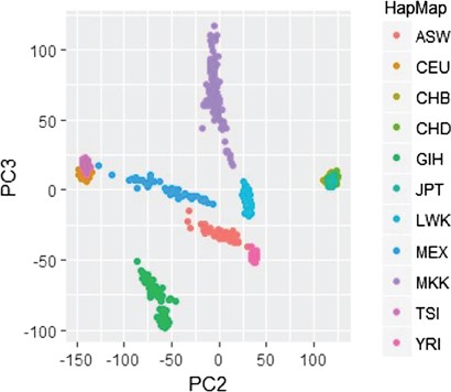
Identifying genetic structure via PCA and HapMap with 11 populations. Linear PCA differentiates 8 subgroups out of 11 populations.
Variations to the classical PCA theme
Robust PCA
In genetics applications, the classical PCA approaches can be greatly influenced by the presence of subject outliers which are probands from an ancestral population that are different from all the other probands. A number of robust PCA approaches to address outliers have been explored and proposed in the literature. However, many of the robust PCA approaches are dependent on the size of samples and number of variables. For example, robust PCA based on minimum volume ellipsoid and minimum covariance determinant requires the sample size to be larger than the number of variables. In contrast, this is not required by the robust PCA based on the projection pursuit (PP) approach, which makes it handle high-dimensional genetics data.
The PP-based robust PCA was first proposed by Li and Chen [90]. However, Liu et al. [18] pointed out that their approach involves a very complicated and difficult algorithm to apply in practice. To increase the practicality of the method improved algorithms have been developed by Croux and Ruiz-Gazen [91] and Croux et al. [92]. Further, Liu et al. [18] considered two algorithms that are more practical and reduce computational time for the PP-based robust PCA using the CR algorithm proposed by Croux and Ruiz-Gazen [91] and the GRID algorithm proposed by Croux et al. [92].
The remaining PCs can be obtained sequentially. This allows one to compute the top PCs with reduced computational time. Details of the algorithm are found in Liu et al. [18]. In the case of performing a PP-based robust PCA to correct for population structure, the steps are (i) to identify outliers using PP-based robust PCA; (ii) to perform regular PCA on the SNP data matrix after removing the identified outliers; (iii) to determine the optimal number of clusters using the selected top PCs in a |$k$|-medoids clustering method; and (iv) to include PCs as covariates and cluster membership as additional factors in regression models as correcting factors for population structure.
Sparse PCA
Even though PCA is widely used in data processing and dimensionality reduction, PCA also has an obvious drawback, that is, each PC is a linear combination of all |$M$| variables and the loadings are typically nonzero. This makes it often difficult to interpret the derived PCs [87]. Zou et al. [87] introduced a new approach called sparse PCA for estimating PCs with sparse loadings. By requiring the PC loading vectors to be sparse, i.e. having a small number of nonzero loadings with the remaining many loadings exactly equalling zero, sparse PCA methods yield PCs that are more easily interpretable [56]. The PCA can be performed via the SVD or EVD of the data matrix. The PCA can also be written as a regression-type optimization problem, which is the basis for the sparse PCA approach. It is noted that the sparse PCA approach does not explicitly impose the uncorrelatedness of PCs and natural ordering of the PCs according to their variances. As a result the PCs may be correlated and unordered. The QR decomposition is used to determine the adjusted explained variances. We refer to Zou et al. [87] for the mathematical details and computational algorithms to fit sparse PCA models, which are implemented in the R package elasticnet.
As an alternative to the approach by Zou et al. [87], Shen and Huang [93] proposed a simpler to implement and computationally less expensive sparse PCA method via regularized SVD (sPCA-rSVD) using the connection of PCA with SVD of the data matrix and extracting the PCs through solving a low-rank matrix approximation problem. Noting that the existing sparse PCA methods are not satisfactory for high-dimensional data applications because they give too many nonzero coefficients, Lee et al. [82] introduced a super-sparse PCA for high-throughput genomic data by modifying nonlinear iterative partial least square (NIPALS) method that is also used for PCA.
Spectral graph theory and PCA
In order to produce a more meaningful delineation of ancestry than by using the classical PCA based on |$X{X}^T$|, Lee et al. [94] considered a spectral embedding derived from the normalized Laplacian of a graph. The method is found to be robust against outliers and can more easily incorporate different similarity measures of genetic data than PCA. Following Belkin and Niyogi [95], Lee et al. [94] defined Laplacian eigenmaps a new representation of the data matrix by decomposing a graph. They used SNP data from the POPRES [96] database to assess the performance of spectral embeddings. Based on the analysis of this dataset that consists of genome-wide SNP panels from African-American, East-Asian, Asian-Indian, Mexican and European origin, Lee et al. [94] showed that the spectral graph approach to PCA performs better than classical PCA yielding a more meaningful delineation of ancestry.
Generalized PCA
The widely used linear PCA basically assumes that the relationships between variables are linear, and its interpretation is only sensible if all the variables are assumed to be continuous [97]. Thus, noting that the linear PCA is not an appropriate method of dimension reduction for categorical (nominal and ordinal) variables like SNP data, various methods of dimension reduction for binary, ordinal and nominal data have been developed in the literature. Landgraf and Lee [98] noted the fact that PCA finds a low-rank subspace by implicitly minimizing the re-construction error under the squared error loss, and its probabilistic interpretation based on normal likelihood allows one to extend the application of PCA to non-Gaussian data such as binary responses and counts [98]. In this regard, Collins et al. [99] proposed a generalization of PCA to the exponential family of distributions using the GLM framework. De Leeuw [100] and Schein et al. [101] considered logistic PCA using the Bernoulli likelihood for binary data, and Lu et al. [102]developed exponential family PCA for categorical data where SNP values are treated as categories using a multinomialdistribution, which is also extended in a supervised framework to supervised categorical PCA (CATPCA). Recently, Song et al. [103] discussed the motivation and rationale of some parametric and nonparametric versions of PCA specifically geared for genomic binary data. Moreover, Lee et al. [56] developed a sparse logistic PCA for binary data extending the method of Shen and Huang [93], an sPCA-rSVD. They demonstrated the effectiveness of the sparse logistic PCA method on SNP data where SNPs are coded as binary as used in dominant and recessive genetics models. On the other hand, Linting et al. [97] discussed CATPCA, which is also referred to as nonlinear PCA for ordinal and nominal variables. The main idea of CATPCA is first to use optimal scaling that converts every categorical variable to a numeric value and then to apply PCA on the quantified categorical variables.
Kernel PCA
As pointed out above, linear PCA may not be appropriate to detect all structure in a genomic dataset. Specifically, if the data are concentrated in a nonlinear subspace, PCA will not be suitable for detecting it. Thus, one may consider kernel PCA, which is the most widely used method among the nonlinear versions of PCA and takes into account nonlinear structures in high-dimensional data. We briefly describe the steps required to extract kernel-based PCs as discussed in [104].
where |${1}_N$| denotes a |$N\times N$| matrix for which each element takes value |$1/N$|.
The kernel based PCs can be obtained using EVD of the centred kernel |${K}_c={U}^{(K)}{D}^{(K)}{U^{(K)}}^T$|, where |${U}^{(K)}$| is a matrix of eigenvectors, and |${D}^{(K)}$| is a diagonal matrix of positive eigenvalues of |${K}_c$|. It follows that the |$j$|th kernel PC score corresponding to |$j$|th eigenvector based on the centered kernel is given by |${z}_j^{(K)}=\sum_{i=1}^N{U}_{ij}^{(K)}{\mathrm{K}}_c\left({x}_i,x\right)$|, |$j=1,\dots, N$|. Detailed derivations of these results are given in [104] among many others.
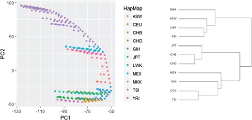
Identifying genetic structure via ncMCE approach on HapMap data (reanalysis). The PC plots ordering and the phylogenetic tree structure agree substantially.
Minimum Curvilinear Embedding
In addition to the common kernel functions–based PCA approaches to capture nonlinear genetic data patterns, Lobato et al. [81] introduced a non-centred Minimum Curvilinear Embedding (ncMCE) approach to population genetics data to explore hierarchical and nonlinear representation of the relationships between and within different populations. The principle behind ncMCE suggests that curvilinear distances between individuals may be estimated as pairwise distances over their Minimum Spanning Tree, constructed according to a selected norm (Euclidean, correlation, etc.) in a high-dimensional feature space. The collection of all nonlinear pairwise distances forms a distance matrix called the MC distance matrix or the MC-kernel. The centred or non-centred versions of MC-kernel can be used as an input to compute PCs.
Consider |$G$| as a matrix of |$N\times M$| genotypes. The steps involved to implement the centred and non-centred MCE-based PCA approach as presented in Lobato et al. [64] are as follows: (i) compute the Euclidean or correlation distance between individuals in |$G$| to generate |$N\times N$| distance matrix |$A$|; (ii) extract the minimum spanning tree out of the distance matrix |$A$|; (iii) compute the distance between all node pairs over the minimum spanning tree to obtain the MC-Kernel, |$K$|; (iv) if centering is required, set |$K=\frac{1}{2}J{K}^2J$| with |$J={I}_N-\frac{1}{2 }{1}_N{1}_N^T$|; (v) perform SVD of |$\tilde{K}={U}^{(MC)}{\Lambda}^{(MC)}{V^{(MC)}}^T$|, where |$\tilde{K}$| is a matrix of |$L\times L$|, |$L<N$|; and (vi) compute scaled scores for each individual, |${Z}^{(MC)}=\sqrt{\Lambda^{(MC)}}{V}^{(MC)}$|; where |${K}^2$| is the matrix of entry-wise squares, |$\tilde{K}$| is the closest approximation to |$K$| by a matrix of rank |$L$| and the others as defined above.
We applied the ncMCE approach on HapMap data. The resulting plots of ncMCE PCs tend to group the 11 HapMap populations almost along their phylogenetic tree. In Figure 4, the phylogenetic tree is constructed by averaging the SNPs of all individuals within a population in order to generate a representative sample and applying hierarchical clustering on the representative samples [64].
Probabilistic PCA
A notable feature of the definition of PCA given by Pearson and Hotelling is the absence of an associated probabilistic model for the observed data [106]. However, PCA can be derived within a density-estimation framework. A probabilistic formulation of PCA from a Gaussian latent variable model that is closely related to statistical factor analysis is obtained by Tipping and Bishop [106]. The authors showed that the principal axes emerge as maximum-likelihood parameter estimates that may be computed by the usual EVD of the sample covariance matrix and subsequently incorporated in the model. Alternatively, the latent-variable formulation leads naturally to an iterative, and computationally efficient, expectation-maximisation algorithm for effecting PCA. Probabilistic PCA has the advantage of estimating the principal axes in cases where some, or indeed all, of the data vectors exhibit one or more missing at random values. Furthermore, in probabilistic PCA, the Bayesian PCA modelling technique is developed to improve upon the accuracy of the estimated PCA model using maximum likelihood approach by incorporating external knowledge about these quantities through a prior density function [107]. Similarly, approaches such as exponential family PCA and nonnegative matrix factorisation have successfully extended PCA to non-Gaussian data types. Moreover, to take advantage of Bayesian inference, Mohamed et al. [108] introduced Bayesian exponential family PCA.
Computational tools used in PCA
A list of software in common use for extracting PCs from genetic data is presented in Table 2.
Software for PCA computation from genetic data
Software for PCA computation from genetic data
Remaining challenges
Missing data
The power of GWAS to identify true genetic associations depends upon the overall quality of the genome-wide SNP data. Genotype missingness is one of the serious issues of data quality that needs attention. In this section we discuss the effect of missing data on PC computation and the role played by PCA in handling missing genotypes. In some applications, certain observations may be missing some variables, and the standard formulas for constructing the eigenvectors or PCs do not apply. There are various imputation methods and software solutions that have been shown to be most promising tools to recover missing genotypes. These include randomForest (R package), which is based on random forest regression for missing genotypes [109, 110]; ranger, which is a fast implementation of random forests for high-dimensional data in C++ and R [111]; and Beagle and IMPUTE2, which are LD-based imputation methods using reference data panels from HapMap or 1000 Genomes Projects. There are also PCA-based imputation procedures such as probabilistic PCA and NIPALS PCA. The PCA-based imputation procedures are implemented in R package pcaMethods [17]. The principle behind these PCA-based imputations is that missing values are initially set to the row averages, and SVD of the SNP matrix is used to create orthogonal PCs. The PCs, which correspond to the largest eigenvalues, are then used to reconstruct the missing SNP genotypes in the SNP matrix [112].
Rare variants
Many recent studies have shifted their focus to rare variants that are more likely to have direct functional impacts on gene products. Because these variants are rare, large sample sizes and cost-effective approaches (such as targeted sequencing of candidate genes or the whole exome) are required to ensure sufficient statistical power [113]. Existing approaches developed for genome-wide SNP data to control for population structure do not work well with modest amounts of genetic data, such as in targeted sequencing or exome chip genotyping experiments. Mathieson and McVean [114] demonstrated that rare variants can show a systematically different and typically stronger stratification than common variants and that this is not necessarily corrected by existing methods such as GC, PCA by simply including the top PCs and mixed models. They also showed that the same process leads to inflation for load-based or burden tests for rare variant association analysis and can obscure signals at truly associated variants. In regard to PCA, they argued that including a large enough number of PCs (between 20 and 100 PCs or highly nonlinear functions) will remove virtually all stratification but it is not possible to know how many PCs are required and inclusion of many components will lead to a substantial reduction in power to detect true associations.
The PCA-based methods have been extended to estimate individual ancestry directly from low-coverage sequencing data when genotypes cannot be accurately estimated [115]. One such method is implemented in LASER 1.0 and LASER 2.0 [113]. LASER first constructs a reference ancestry space by applying PCA to the genotype data of the reference individuals. Then, genome-wide sequence reads for each sequence sample are analysed to place the sample into the reference PCA space. The estimated coordinates of the sequence samples can reflect their ancestral background and can be used to correct for PS in association studies. In addition to estimation of individual ancestry using sequence reads, LASER also provides an option to perform standard PCA on genotype data. This option is implemented to prepare the reference PCA coordinate file as an input for LASER. It can also be used independently as a PCA tool for analysing population structure based on SNP genotypes.
Fumagalli et al. [116] noted that accuracy in identifying population structure can be recovered when calling genotypes by removing outlier individuals, low-quality sites and low-frequency variants, but at the price of losing potential important information. As a remedy, they proposed a method that weighs each site according to its probability of being variable instead of using an arbitrary discrete SNP calling, or minor allele frequency, cut-off. Thus, for genotype calls from low or moderate coverage next generation sequencing data, they showed that population structure can be investigated with PCA under a probabilistic framework that accounts for sequencing errors. Their approach resulted in a weighted version of the covariance matrix estimation presented in [32].
Some recent progresses on PCA variations in statistical genetics
| Methods | References |
|---|---|
| Logistic PCA for binary data | Songet al.[131] |
| Exponential family PCA | Mohamedet al.[136] |
| CATPCA for nominal data | Luet al.[173] |
| Kernel or nonlinear PCA | Popescuet al.[75] |
| Sparse (logistic) PCA | Leeet al.[42] |
| Sparse exponential family PCA | Luet al.[130] |
| Robust PCA for outlier detection | Liuet al.[24] |
| Fast PCA for large datasets | Abrahamet al.[81] |
| PCA for related samples (PC-Relate) | Conomoset al.[18] |
| PCA to capture phylogenetic structure | Alanis-Lobatoet al.[174] |
| PCA to impute missing genotypes | Stacklieset al.[23] |
| PCA to handle rare variants | Mathiesen and McVean [138] |
Families or related samples
Many genetic studies include individuals with some degree of relatedness, and existing methods for inferring genetic ancestry fail in related samples [117]. With related individuals, correlations among relatives must be taken into account to ensure the validity of the test and to improve power [118]. Several methods have been proposed for case–control association testing in related samples from a single population with known pedigrees [118] or unknown relationships [119]. In the presence of population structure for related samples, Thornton and McPeek [120] proposed a method called ROADTRIPS. ROADTRIPS uses an empirical covariance matrix calculated from genome-screen data to correct for unknown population and pedigree structure while maintaining high power by taking advantage of known pedigree information when it is available [120].
In recent papers, Conomos et al. proposed two methods based on PCs: PC-AiR for population structure inference in the presence of genetic relatedness, known or cryptic, among sampled individuals and PC-Relate for accurate relatedness estimation in the presence of population structure [13, 117]. The PC-AiR uses measures of pairwise relatedness (kinship coefficients) as well as measures of pairwise ancestry divergence based on genome-screen data together with an efficient algorithm to identify a diverse subset of unrelated individuals that is representative of all ancestries in the sample. Then a standard PCA is performed on this ‘unrelated subset’ of individuals, and PC values for all remaining are predicted based on genetic similarity [117]. The PC-Relate method is a model-free approach for estimating commonly used measures of recent genetic relatedness, such as kinship coefficients and IBD sharing probabilities, in the presence of unspecified structure. It uses ancestry representative PCs obtained via PC-AiR to account for sample ancestry differences and to provide estimates that are robust to population structure, ancestry admixture and departures from HWE [13]. Both PC-AiR and PC-Relate are implemented in the R package GENESIS.
In addition, an increasing number of hybrid approaches have entered the scene. One of these was proposed by Li et al. [121] and combines information from multidimensional scaling and phylogenetic trees to correct for PS in unrelated individuals. Another hybrid approach combines to combining evidences from both families and unrelated samples [122]. In the unified approach by Zhu et al. [122], first PCA is performed on unrelated individuals and founders of families where both trait and test marker data are corrected for PC background via linear regression as suggested by Price et al. [10]. Then PCs are projected on family members, whenever these are available, and residuals from the Price linear regressions are computed. Finally, the authors propose a one degree of freedom chi-squared test statistic that reduces to the test statistic of Price et al. [10] when the sample only consists of unrelated individuals. Another hybrid approach considered in Solovieff et al. [57] is to first select the most informative PCs for cluster analysis, to use a cluster algorithm to identify population substructure and to compute a ‘scoring index’ to automatically select the best number of clusters. Second, identified number of clusters is used in an SA method. Hints towards such a hybrid approach were given in Ziegler and König [123].
Meta-analysis
In the context of meta-analyses for GWAs, either GC- or PC-based methods are adopted to control spurious associations between genetic variants and disease that are caused by PS. A double GC correction is required since the combined statistics across the genome need to be adjusted with a corresponding inflation factor. Double GC correction for PS in the meta-analysis for GWAS has been implemented in the software METAL [124] and GWAMA [125]. The PCA correction method that adjusts for stratification involves incorporating top PCs of genotype data as covariates in parametric regression models and then to combine beta coefficients and standard errors from these study-specific PC adjusted regression results [126]. Wang et al. [127] showed that PCA correction is more effective than the double GC correction in meta-analysis. Notably, simply including population as a covariate in the meta-analysis is not always an effective substitute for analyzing the subpopulations separately [128]. They may reveal population-specific signals, which were also indicated by Keen-Kim et al. [129].
Epistasis
Although several comparative studies or reviews are available (including Setakis et al. [130], Astle and Balding [131], Price et al. [65], Bouaziz et al. [132], Sillanpää [133]), additional work is needed to investigate the relative merits of the different statistical analysis techniques that are able to eliminate the effects of PS in genetic main effects association studies, while including both commonly and non-commonly used approaches. Often, simulation results heavily depend on the true underlying (risk) models and the underlying population structure (e.g. even when comparing GC with SA: Wawro et al. [134]), despite them attributing overall good performance to PCA-based approaches. Since neither the true underlying population structure nor the genetic mode of inheritance or the genetic effect is known, controlling for potential confounding by PS or admixture remains a challenging task. This is also indicated by the continuing flow of new methods and comparative studies on the topics. In addition, with a gradual shift from single locus GWAS to genome-wide gene–environment and gene–gene interaction searches more attention needs to be given to the effects of PS on genome-wide interaction studies. For instance, there is a problem with tests of gene–environment interaction when the marker being tested is associated with disease risk, but is not in itself the causal variant [135]. In gene–gene interaction studies where the marginal effects of genes are not prominent and the cumulative effects of genes are quite small, the PS can cause even more dramatic deviation from the real situation. In the context of gene–gene interaction studies Bhattacharjee et al. [136] pointed towards the potential powerful role of PCA in the exploration of gene–gene interactions in case–control studies. This idea and the ideas of Price et al. [10] were combined in a novel Multifactor Dimensionality Reduction approach to detect gene–gene interactions [14]. In effect, adjusting both phenotype and genotype for genetic background as above can also be combined with filtering approaches such as Random Forests [137]. Forest-based ensemble approaches are often used in gene–gene interaction studies to reduce the number of interactions to test for [138]. Our group has been at the cradle of Model-Based Multifactor Dimensionality Reduction Method (MB-MDR) developments (e.g. Calle et al. [139], Cattaert et al. [140], Gola et al. [141]). Since to date, MB-MDR can only deal with categorical marker data; adopting a similar approach as in Niu et al. [14] is not possible. Hence, a PCA-based correction for PS with MB-MDR can either be achieved by a priori trait adjustment for genetic background, prior to data submission to MB-MDR, or a correction during internal MB-MDR association testing. Both are far from ideal: where the first involves a differential adjustment of traits and SNPs, the second is computationally demanding. A polygenic background correction of traits prior to MB-MDR analysis will inherit some of the advantages of mixed modeling over PCA but is expected to inadequately maintain type I error in the presence of population structure or admixture.
When data become bigger than big
With the advancement of new technologies and a reduction in cost of sequencing, in recent years the size of samples in sequencing has increased, which brings a huge increase in the size of SNP datasets. This in turn makes it time-consuming to perform classical PCA using, for example, EIGENSOFT on large datasets involving millions of genotypes and tens of thousands of individuals. In recent years, alternative approaches of performing PCA have been introduced using randomized matrix algorithms that provide the top PCs with high-accuracy relative to the traditional methods [63, 66]. Since in genomic analysis many of the tools are based on the first few PCs, these algorithms are very useful and computationally tractable for large datasets. Abraham and Inouye [63] summarized the randomized matrix implementation of PCA as follows. First a relatively small matrix is constructed that captures the top eigenvalues and eigenvectors of the original data, with high probability. Next, standard SVD or EVD is performed on this reduced matrix, producing nearly identical results to what would have been achieved using a full analysis of the original data. In this regard, Abraham and Inouye [63] proposed the flashpca algorithm, which is an efficient tool for performing PCA on large genome-wide data, based on randomized algorithms. They demonstrated the accuracy and speed of flashpca on both HapMap3 and on a large Inmmunochip dataset. Similarly, Galinsky et al. [66] proposed Fastpca algorithm, which is found much faster than flashpca.
Finally, in Table 3, we give a summary of the recent developments of PCA variants presented in this review.
In conclusion
PCA has a long tradition in multivariate exploratory statistical analyses. With the availability of large panels of genetic markers, and the seminal paper of Novembre and Stephens [9] showing that PCs based on selected markers can adequately capture genetic variation following geographic country-of-origin sample distributions, PCA became the mainstream instrument to describe population structure using molecular markers or to capture confounding by shared genetic ancestry in GWAS. Less work has been devoted to their role in genome wide association interaction studies (GWAIS), for which multiple analytic approaches exist to detect epistasis outside a regression framework. Also, little is known about the occurrence or importance of nonlinear similarities between individuals and its impact on GWAS/GWAIS. Although investigating the latter was outside the scope of this paper, we have paved the way to considering alternative flavours of PCs in genetic studies.
PCA has enjoyed great popularity in various applications as a valuable tool for data dimension reduction and data visualization.
In statistical genetics, PCA appears in the context of GWAS where PCs become the mainstream instrument to describe population structure using molecular markers or to capture confounding by shared geneticancestry, prediction analyses and data dimensionality reduction.
This review of PCA in statistical genetics using SNPs as a statistical markers focuses on different aspects of the classical PCA: computational issues, practical considerations and its modifications and extensions.
The review also includes recent advances of PCA methods and software that deal with large-scale data sets, family data, nonlinearity, sparsity, data integration, meta-analysis, epistasis and rare variants.
As a comprehensive review of existing works of PCA, it is our belief that this paper will provide valuable insight and pave the way to considering alternative flavours of PCs in genetic studies.
Funding
This research was in part funded by the Fonds de la Recherche Scientifique (FNRS), in particular ‘Integrated complex traits epistasis kit’ (Convention n° 2.4609.11) [K.V.S., J.M.J., E.G.]. We also acknowledge research opportunities offered by FNRS, including ‘Foresting in Integromics Inference’ (Convention n° T.0180.13) [K.C.], and by the interuniversity research institute Walloon Excellence in Lifesciences and BIOtechnology (WELBIO) [F.A., K.V.S.], by the German Research Foundation (DFG, FOR488 grant no. KO2250/5-1 and KFO303 no. KO2250/7-1) and by the German Federal Ministry of Education and Research (Bundesministerium für Bildung und Forschung, BMBF) as part of funding for the German Center for Lung Research (DZL) and the German Center for Cardiovascular Research (DZHK) [I.R.K.].
Fentaw Abegaz is a postdoctoral researcher at the University of Liège (Belgium). He works on the development and amelioration of epistasis detection strategies, multivariate analysis and dynamic network reconstruction.
Kridsadakorn Chaichoompu is a postdoctoral researcher at Max Planck Institute of Psychiatry (Germany). His main interest is about development of bioinformatics methodologies.
Emmanuelle Génin is a research director at Inserm in Brest (France). Her research interests are the development and the evaluation of methods derived from population genetics to evidence genes involved in complex diseases.
David W. Fardo is an Associate Professor of Biostatistics at the University of Kentucky (USA). Much of his research focuses on statistical genetics and neurodegenerative disease.
Inke R. König is Professor for Medical Biometry and Statistics at the Universität zu Lübeck, Germany. She is interested in genetic and clinical epidemiology and published over 220 refereed papers.
Jestinah Mahachie John received the Ph.D. degree in Statistical Genetics from the University of Liege, Belgium. She is currently working as a Senior Statistician at Veramed Ltd in London, UK.
Kristel Van Steen is a Professor at the University of Liège working on Systems Genetics. Her main interest lies in methodological developments related to interactome and integrated analyses to enhance precision medicine.
References
