


Abstract
To detect differentially expressed genes (DEGs) in small-scale cell line experiments, usually with only two or three technical replicates for each state, the commonly used statistical methods such as significance analysis of microarrays (SAM), limma and RankProd (RP) lack statistical power, while the fold change method lacks any statistical control. In this study, we demonstrated that the within-sample relative expression orderings (REOs) of gene pairs were highly stable among technical replicates of a cell line but often widely disrupted after certain treatments such like gene knockdown, gene transfection and drug treatment. Based on this finding, we customized the RankComp algorithm, previously designed for individualized differential expression analysis through REO comparison, to identify DEGs with certain statistical control for small-scale cell line data. In both simulated and real data, the new algorithm, named CellComp, exhibited high precision with much higher sensitivity than the original RankComp, SAM, limma and RP methods. Therefore, CellComp provides an efficient tool for analyzing small-scale cell line data.
Introduction
Gene expression profiles with only two or three technical replicates are commonly used for detecting differentially expressed genes (DEGs) in a cell line after a certain treatment, given that there is no biological difference among technical replicates derived from a particular cell clone population. Current statistical methods such as the significance analysis of microarrays (SAM) [1] and Student’s t-test often have insufficient statistical power for this application scenario. More frequently, researchers use the fold change (FC) metrics, calculated as the ratios of the average gene expression levels between the treated and untreated cell lines, to detect the genes with FC values greater than an arbitrary preset threshold as DEGs [2–4]. However, this method does not provide any statistical control. Obviously, the lowly expressed genes in both conditions may easily have large FCs simply because of technical variations [1, 5, 6] and the highly expressed genes in both conditions can hardly have large FCs [7]. To address this problem, we have proposed an algorithm to identify DEGs based on the significant reproducibility of genes with top-ranked FCs or average expression differences (ADs) between paired case-control replicates [7]. However, it still cannot obtain DEGs with false discovery rate (FDR) control.
Recently, we developed another algorithm, RankComp [8], to identify DEGs in an individual disease sample through finding those genes whose upregulations or downregulations can lead to the observed disrupted relative expression orderings (REOs) of gene pairs within this sample, taking the highly stable REOs predetermined in a large collection of samples for the corresponding normal tissues as the background. Owing to the large interindividual expression variations of human tissue samples, it is necessary to use a large number of previously accumulated normal samples to establish the stable normal REOs landscape for a particular type of human tissue [9, 10]. In contrast, there exist only measurement variations among technical replicates of a cell line. Thus, it is possible that two or three technical replicates are sufficient for constructing the stable REOs landscape of samples for a cell line. Given the above consideration, if a treatment widely disrupts the stable REOs found in untreated cell lines, RankComp should be also applicable to detect DEGs between the treated and untreated cell lines. RankComp adopts a filtering process to reduce the potential effects of the upward (or downward) expression changes of other genes on the downregulation or upregulation determination of a gene. However, as described in the ‘Methods’ section, this filtering process cannot minimize the potential effects of other genes confounding the REOs comparison for a particular gene, which tends to reduce the sensitivity of the algorithm.
In this study, using seven small-scale data sets for human cancer cell lines, we demonstrated that the REOs of gene pairs were highly stable among the technical replicates of a particular cell line but were widely disrupted after a certain treatment. Further, we improved the core algorithm of RankComp and customized it to the identification of DEGs for small-scale cell data with only two or three technical replicates. The new algorithm, called CellComp, showed much higher sensitivity than the original RankComp algorithm, the commonly used SAM [1], limma [11, 12] and RankProd (RP) [13] methods as evaluated in both simulated and real data.
Material and methods
Data and preprocessing
Seven small data sets for proliferation analyses of human cancer cell lines were obtained from Gene Expression Omnibus (GEO, http://www.ncbi.nlm.nih.gov/geo/) and ArrayExpress (http://www.ebi.ac.uk/arrayexpress/), as described in Table 1, which were used to evaluate the reproducibility of REOs among technical replicates of a cell line and compare the performances of differential expression analysis methods. Another large data set from GEO (Table 1) was used to evaluate the performance of CellComp in small subsets derived from the full data set, taking the DEGs detected from the full data set by SAM as the benchmark. For the data measured by the Affymetrix platform, the raw data (.cel files) were downloaded and normalized using the Robust Multichip Average algorithm [14]. For the data measured by the Agilent and Illumina platforms, the normalized data were downloaded. Probe IDs were mapped to gene IDs using the corresponding platform files. If multiple probes were mapped to the same gene, the arithmetic mean of the values of the multiple probes was used as the expression value of this gene. For the RNA sequencing (RNA-seq) data, the raw counts, the fragments per kilobase of transcript per million fragments mapped (FPKM) and the transcripts per million (TPM) values were downloaded. The genes with nonzero counts, nonzero FPKM and nonzero TPM values in all samples were analyzed.
Data sets for human cancer cell lines analyzed in this study
| Data accession | Cell line | Cancer type | Treatment | Size |
|---|---|---|---|---|
| GSE29084 | HepG2 | Liver cancer | HNF4A knockdown | 2 VS 2 |
| GSE38581 | MKN45 | Gastric cancer | Hsa-miR-29c transfection | 2 VS 2 |
| GSE38581 | MKN74 | Gastric cancer | Hsa-miR-29c transfection | 2 VS 2 |
| GSE31450 | SNU638 | Gastric cancer | LAP2β transfection | 3 VS 3 |
| E-MEXP-1691 | HCT116 | Colon cancer | 5-FU-treatment for 24h | 3 VS 3 |
| GSE35004 | Hep3B | Liver cancer | YAP knockdown | 3 VS 3 |
| GSE78167 | MCF7 | Breast cancer | Estrogen-treatment for 2h | 3 VS 3 |
| GSE15709 | A2780 | Ovarian cancer | Cisplatin-induced resistance | 5 VS 5 |
Stable REOs
In each sample, the REO of a gene pair (i and j) is denoted as either Gi > Gj or Gi < Gj exclusively, where Gi and Gj represent the expression values of gene i and j, respectively. Among a large set of samples of a state, whether the REO of a gene pair is stable or not is tested using the binomial test as described in the original RankComp algorithm [8]. However, this test is not applicable to cell line data sets, where the sample size is small. For example, the probability to observe the same REO by chance is 1/2 among two technical replicates and 1/4 among three technical replicates under the hypothesis that a certain REO outcome (Gi > Gj or Gi < Gj) has a probability of 1/2 to occur. This hypothesis is true for those genes with the same or close expression levels, but random measurement noise may lead to different observed REOs. To address this problem, we made two modifications to identify stable REOs under each treatment state, respectively. First, the REO of a gene pair must be identical among all the samples under one treatment state. Second, a parameter, e, is set in the judgment of stable REOs: a certain percentage (e.g. 5, 15 or 25%) of gene pairs, among all gene pairs in building the background stable gene pairs, that have the smallest rank differences in each sample are excluded. In principle, the parameter e should be associated with the measurement variation which is dependent on the expression levels [15]. However, the variation level for each gene is hard to be measured. Thus, we did simulation experiments to evaluate the influence of e setting as described in ‘Results’ section.
For the microarray data, the gene expression values can be directly used to evaluate REOs of gene pairs. For the RNA-seq data, reads per kilobase per million (RPKM), FPKM and TPM, which normalize the gene transcription length and the sequencing depth [16–18], can represent the actual gene expression abundance and thus can be applied to rank gene expression levels. However, the count value of a gene is proportional not just to the expression level of this gene but also to its gene transcript length and to the sequencing depth and counts per million only considers sequencing depth [19, 20], and thus these metrics are not suitable to rank gene expression levels.
The CellComp algorithm to detect DEGs
Figure 1 describes the flowchart for CellComp. First, with a presettled parameter e, stable gene pairs, which have identical REOs in all replicates of State 1 (here, the untreated samples) and State 2 (here, the treated samples) are obtained, respectively. The comparison of REOs between the two states is limited to the scope of the overlapped gene pairs of the two lists of stable gene pairs, defined as the background gene pairs. The gene pairs with unstable REOs in any of the two cell states are discarded to minimize the influence of random experimental factors.
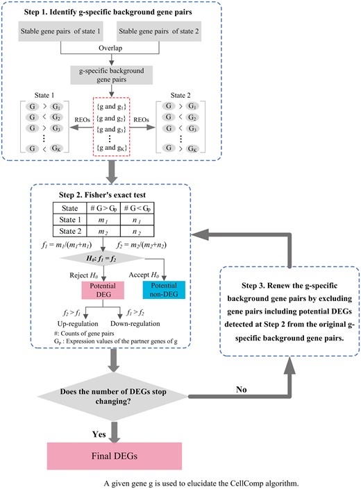
The flowchart for the CellComp algorithm. We use a given gene g to elucidate this algorithm. The first step is to extract the g-specific background gene pairs, each including g, which are stable in both State 1 and State 2. The second step is to perform Fisher’s exact test to test the null hypothesis that f1 and f2 are equal, where f1 and f2 denote the frequencies of gene pairs, among all g-specific background gene pairs, in which g shows a higher expression level than its partner genes in State 1 and State 2, respectively. After all genes are judged as potential DEGs or non-DEGs, the third step is to renew the g-specific background gene pairs. Only the gene pairs each including g and potential non-DEGs identified from Step 2 are retained. Step 2 and Step 3 are repeated until the number of detected DEGs stops changing.
For a given gene g, all the gene pairs including g are defined as g-specific background gene pairs. Let f1 and f2 denote the frequencies of the gene pairs in which g shows a higher expression level than its partner genes in State 1 and State 2, respectively, among all g-specific background gene pairs. Fisher’s exact test is used to test the null hypothesis that f1 and f2 are equal. If the null hypothesis is rejected at a given significance level, g is judged as a potential DEG: if f2 > f1, suggesting that the expression level of g is higher than significantly more genes in State 2 than in State 1, g is judged as upregulated, otherwise, downregulated. The Benjamini–Hochberg procedure was used to control FDR in the multiple tests. This is a concise description for the Fisher’s exact test in the original RankComp algorithm [8]. After all genes are judged as potential DEGs or non-DEGs, a filtering process is iteratively performed to minimize the influence of other genes’ expression changes on the Fisher’s exact test for a particular gene. For each gene g, the g-specific background gene pairs are renewed by excluding gene pairs composed with g and those potential DEGs detected in the previous step, and Fisher’s exact test is performed again. This filtering process is iteratively performed until the number of DEGs, both the upregulated and downregulated, stops changing.
When genes are widely altered in a cancer cell line by a certain treatment, the upregulation or downregulation of a gene g could be falsely indicated by its paired potential DEGs. To reduce this confound effect, the iterative process is designed to use those potential non-DEGs involved in the g-specific background gene pairs to determine whether g is differentially expressed. In another perspective, if the expression level of g’s paired gene (gp) is not differentially expressed between two cell states, the reversal REO pattern of (g, gp) must result from the differential expression of g. The above filtering process fixes two potential defects of the original RankComp algorithm. First, the filtering process of RankComp adjusts the gene-specific background gene pairs for a given gene g by excluding gene pairs composed with g and only those potential DEGs with the opposite dysregulation direction of g detected in the previous step. This is based on the consideration that only the downregulated or upregulated genes could falsely indicate the upregulation or downregulation of g. However, this unbalanced practice may decrease the chance of selecting g as a DEG because the potential DEGs with the same dysregulation direction of g tend to form nonreversal REOs with g, which is biased to indicate that g is unchanged. Second, RankComp performs only one filtering step, which reduces only partially the influence of other genes’ expression changes on the Fisher’s exact test for a particular gene.
The CellComp and the original RankComp algorithms are implemented in C language for efficiency and tested on Linux, which are freely available online at https://github.com/pathint/reoa. All the other statistical analyses are performed with the aid of the R language package version 3.2.3.
Concordance score
Similarly, if two lists of DEGs identified by two methods in a data set have k overlaps, among which s genes have the same dysregulation directions (upregulation or downregulation) in the two DEGs lists, the concordance score s/k is used to evaluate the consistency of DEGs between the two lists. The frequently used percentage of overlapping genes between two lists of DEGs will be apparently low when any of the two methods in comparison has insufficient power to detect all DEGs in a data set [21]. Here, the cumulative binomial distribution is used to evaluate the probability of observing a concordance score of s/k by chance.
Performance evaluation
In the real data analysis, we evaluated the precision of a DEG identification method according to the concordance score between the identified upregulation or downregulations and the observed upregulated or downregulated directions judged directly by the expression values between the treated and untreated cell lines. If a gene was identified as an upregulated (or downregulated) DEG in treated cell line samples, its average expression level in the treated cell line samples should be larger (or smaller) than that in the untreated cell line samples. Apparently, this criterion serves a necessary but not sufficient condition for a gene to be DEG.
Functional enrichment analysis
Functional enrichment analyses were performed based on gene ontology (GO) [22]. The hypergeometric distribution was used to calculate the statistical significance of biological pathways enriched with genes of interest [23]. The Go-function algorithm was adopted to reduce the redundancy pathways [24]. The Benjamini–Hochberg procedure was used to estimate FDR.
Results
Reproducible REOs of gene pairs among technical replicates of a cell line
Seven data sets for human cancer cell lines, HepG2 [4], MKN45, MKN74 [3], SNU638 [25], HCT116 [26], Hep3B [27] and MCF7 [28] (Table 1), were used to evaluate the reproducibility of REOs of gene pairs among technical replicates of a cell line. We labeled the untreated and treated cell line samples with their GEO or ArrayExpress accession numbers in each data set, as described in Table 2 and Supplementary Table S1.
GEO or ArrayExpress accession numbers of the untreated samples
| Data set | Untreatment 1 | Untreatment 2 | Untreatment 3 |
|---|---|---|---|
| HepG2 | GSM720616 | GSM720618 | – |
| MKN45 | GSM945747 | GSM945748 | – |
| MKN74 | GSM945751 | GSM945752 | – |
| SNU638 | GSM781665 | GSM781666 | GSM781667 |
| HCT116 | S0114F032 | S0114F040 | S0114F042 |
| Hep3B | GSM860172 | GSM860173 | GSM860174 |
| MCF7 | GSM2068643 | GSM2068653 | GSM2068663 |
In the HepG2 data set with two technical replicates in the untreated state, 95.32% of all the 205 689 903 possible gene pairs showed the same REOs in both untreated replicates. That is, the concordance score is 95.32%. Similarly, the concordance scores of the REOs between two untreated replicates were 96.55 and 96.69% in the MKN45 and MKN74 data sets, respectively. The stable REOs detected in small data (here two technical replicates) might include some falsely ‘stable’ REOs observed by random chance. If it does exist stable REOs in technical replicates of a cell line, then the stable REOs detected in small data will be increasingly reproducible in additional samples. To test this assumption, we evaluated the concordance scores stepwise using the data sets with three technical replicates. For three pairs of samples formed by the three untreated replicates from the SNU638 data set, with sample numbers described in Table 2, the concordance scores of the REOs were 93.74% for the paired Samples 1 and 2, 93.36% for the paired Samples 1 and 3 and 94.04% for the paired Samples 2 and 3. As expected, 96.62, 97.01 and 96.31% of the consistent REOs in the three paired replicates, respectively, were reproducible in the third remained replicate for each pair. Similar results were observed in the HCT116, Hep3B and MCF7 data sets (Supplementary Results). These results were highly unlikely to happen by chance (binomial test, all P < 1.11E-16). Highly stable REOs were also observed in the treated cell line samples in each of these data sets (Supplementary Results).
For each data set, all measured genes were involved in the stable gene pairs obtained from the technical replicates of a cell line, indicating that widely stable gene expression ranking is an inherent feature of a cell line in a state. Besides, millions of the background stable REOs in the untreated cell line samples were reversed in the treated cell line samples, making it possible to identify DEGs through REO comparison between the treated and untreated cell lines.
Performance tests on null data sets
We first tested our method on the null data sets, where no DEGs were expected. From each of the above seven data sets, a null data set with the same sample sizes as the original data set was created through adding Gaussian noise to the mean log2-transformed expression value of each gene in all the untreated samples. The variances of technical noises in the original data sets were estimated with a previously proposed method [29] based on the assumption that the measurement noise is intensity dependent [15] and the noises of genes with similar log2-transformed intensities have independently and identically normal distribution. By dividing all genes into bins, each with 200 genes with similar expression levels, this method quantifies the variance of the normal noise distribution by calculating the mean variance of 200 genes in each bin, which can provide a good estimate for parameters of the noise distribution [29]. Then, CellComp was applied to each simulated data set to detect DEGs. The experiments were repeated 1000 times for each of the seven cell lines.
In the null data sets based on the SNU638, HCT116, Hep3B and MCF7 data each with three technical replicates, on average, 10.07, 5.68, 0.41 and 1.37 DEGs were identified by CellComp with FDR < 5%, respectively. The results indicate that the method will detect minimum number of false discoveries in the null data sets with three technical replicates. However, in the null data sets based on the HepG2, MKN45 and MKN74 data each with two technical replicates, 3506.26, 2802.05 and 2605.12 DEGs were identified by CellComp with the same FDR control, respectively, which indicated that there might be too many gene pairs with falsely stable REOs detected by chance in data sets with two replicates. To address this issue, we introduced a parameter, e, to filter out a certain percentage of gene pairs with the closest expression levels in each sample (see ‘Methods’ section). By setting e from 5 to 25%, the numbers of false DEGs decreased sharply, and the numbers became acceptably small in all simulated data sets when e was set at 25% (Table 3). Therefore, 25% was used in the following analyses of data sets with two replicates.
The average numbers of DEGs identified from the null data sets based on the HepG2, MKN45 and MKN74 data each state with two technical replicates
| e (%) | Null data set | ||
|---|---|---|---|
| HepG2 | MKN45 | MKN74 | |
| 5 | 2231.35 | 1689.44 | 1837.88 |
| 15 | 18.16 | 326.85 | 373.11 |
| 25 | 0 | 32.32 | 31.05 |
| e (%) | Null data set | ||
|---|---|---|---|
| HepG2 | MKN45 | MKN74 | |
| 5 | 2231.35 | 1689.44 | 1837.88 |
| 15 | 18.16 | 326.85 | 373.11 |
| 25 | 0 | 32.32 | 31.05 |
Additionally, we evaluated the performance of CellComp with a 10% increase of the SDs of Gaussian noise estimated from the untreated samples for each cell line. On average, 16.09, 11.36, 2.99, 7.38, 0, 51.97 and 50.91 DEGs were identified in the null data sets based on the SNU638, HCT116, Hep3B, MCF7, HepG2, MKN45 and MKN74 data, respectively. The result suggested that the algorithm could tolerate higher noise levels than the estimated ‘actual’ noise levels. Obviously, when the noise level is high, the FC method will inevitably find many false DEGs with large FCs by random chance.
Performance of comparisons in simulated data
We performed simulation experiments based on the expression profiles of two and three untreated cell line samples for the HepG2 and SNU638 data sets, respectively. For each of the two cell lines, the expression profiles of two and three mocked treated samples were generated by randomly selecting 4000 genes, and changing their measured values in each of the untreated samples with FC levels of 1.4, 1/1.4, 1.6, 1/1.6, 1.8, 1/1.8, 2 and 1/2, 500 genes were assigned for each FC level, while the measured values of the rest genes were kept unchanged. The FC levels were calculated based on the expression values without log-transformation, which can represent more institutively the change magnitude than log-FC [5]. The methods, CellComp, RankComp, SAM, limma and RP, were applied to identify DEGs between the simulated treated and untreated samples with FDR < 1, 5 and 10%, respectively. The simulation experiments were repeated 100 times for each cell line data.
As shown in Table 4, CellComp had higher average sensitivity scores than the other methods at each FDR level, while the average specificity scores were ∼1. When FDR was increased from 1 to 10%, the ranges of average sensitivity of CellComp increased from 70.9 to 79.8% in the simulation experiments based on the HepG2 data and from 95.6 to 97.0% in the simulation experiments based on the SNU638 data, whereas the corresponding ranges of average sensitivity of RankComp were 62.8–75.5% and 73.6–75.5%, respectively. Apparently, RP failed to identify any DEG for the simulated data at FDR < 1%, while limma performed worse than CellComp but better than SAM and RP at each FDR control, especially, in the simulated data with three replicates.
Sensitivity, specificity and F-score of DEGs identified by CellComp, RankComp, SAM, limma and RP for simulated data
| FDR (%) | Evaluation | HepG2 | SNU638 | ||||||||
|---|---|---|---|---|---|---|---|---|---|---|---|
| CellComp | RankComp | SAM | limma | RP | CellComp | RankComp | SAM | limma | RP | ||
| 1 | Sensitivity | 0.709 | 0.628 | 0 | 0.025 | 0 | 0.956 | 0.736 | 0.475 | 0.648 | 0 |
| Specificity | 1 | 1 | 1 | 1 | 1 | 0.999 | 0.999 | 1 | 1 | 1 | |
| F-score | 0.829 | 0.772 | 0 | 0.049 | 0 | 0.977 | 0.848 | 0.644 | 0.786 | 0 | |
| 5 | Sensitivity | 0.726 | 0.644 | 0.041 | 0.197 | 0.015 | 0.965 | 0.744 | 0.635 | 0.878 | 0.288 |
| Specificity | 1 | 1 | 1 | 1 | 1 | 0.999 | 0.999 | 1 | 1 | 1 | |
| F-score | 0.842 | 0.784 | 0.079 | 0.328 | 0.029 | 0.982 | 0.853 | 0.777 | 0.935 | 0.447 | |
| 10 | Sensitivity | 0.798 | 0.755 | 0.345 | 0.393 | 0.058 | 0.970 | 0.755 | 0.802 | 0.936 | 0.506 |
| Specificity | 1 | 1 | 0.994 | 1 | 1 | 0.999 | 0.999 | 1 | 1 | 1 | |
| F-score | 0.888 | 0.860 | 0.508 | 0.564 | 0.109 | 0.984 | 0.860 | 0.890 | 0.967 | 0.672 | |
Performance comparisons in real data
Seven real data sets, HepG2, MKN45, MKN74, SNU638, HCT116, Hep3B and MCF7, were used to further evaluate the performance of CellComp, SAM for microarray data or SAMseq [30] for RNA-seq data, limma and RP (Figure 2). To identify DEGs for RNA-seq data, the input data of SAMseq [30] and voom/limma [20] should be the count values. For the data sets with two technical replicates, we set e at 25% to minimize the falsely stable REOs. In the HepG2, MKN45 and MKN74 data sets, the concordance scores of the REOs between two untreated replicates increased from 95.32 to 99.27%, 96.55 to 99.72% and 96.69 to 99.86%, respectively, after controlling e. All measured genes were also involved in the stable gene pairs obtained from the technical replicates of a cell line after controlling e. With FDR < 5%, there were 1335, 849, 941, 1323, 1067, 753 and 2949 DEGs detected by CellComp from the seven data sets, respectively.
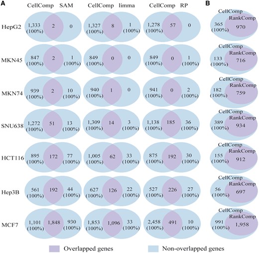
Concordance analyses of the detected DEGs. The precision of DEGs is marked in the brackets. (A) The concordance of DEGs identified by CellComp and SAM (or SAMseq), limma or RP. (B) The concordance of DEGs identified by CellComp and RankComp.
In the three data sets with two technical replicates, there were only 0–57 DEGs detected by SAM (with 1000 permutations), limma and RP (with 1000 permutations) with FDR < 5%. In the SNU638 data set with three technical replicates, SAM, limma and RP found 64, 17 and 221 DEGs, respectively, and 79.69% (51), 82.35% (14) and 83.71% (185) of these DEGs were also detected by CellComp. In contrast, 96.15% (1272), 98.94% (1309) and 86.02% (1138) of the DEGs identified by CellComp were missed by SAM, limma and RP, respectively, and the apparent precision of these DEGs was 100% according to the observed average differences between the treated and untreated cell lines in each data set. In the HCT116 data set with three technical replicates, SAM, limma and RP found 249, 95 and 222 DEGs, respectively, and 69.08% (172), 65.26% (62) and 86.49% (192) of these DEGs were also detected by CellComp. In contrast, 83.88% (895), 94.19% (1005) and 82.01% (875) of the DEGs identified by CellComp were missed by SAM, limma and RP, respectively, and the precision of these DEGs was also 100%. Similar results were also observed in the Hep3B data set (Figure 2A). In the MCF7 data set with the count, TPM and FPKM values, we first compared the performance of CellComp based on the TPM and FPKM values. With FDR < 5%, CellComp identified 2949 and 2980 DEGs based on FPKM and TPM, respectively. The two DEGs lists had 2936 overlaps and 100% of these genes had the same dysregulation directions across the two lists, suggesting that using TPM and FPKM to rank the genes, CellComp generates almost the same result. Then, we compared the performance of CellComp using TPM or FPKM with SAMseq, voom/limma and RP. Notably, the input data should be the count values when applying SAMseq [30] and voom/limma [20] to RNA-seq data. With FDR < 5%, SAMseq, voom/limma and RP (with TPM values) found 2777, 1129 and 501 DEGs, respectively, and 66.55% (1848), 97.08% (1096) and 98.00% (491) of these DEGs were detected by CellComp. In contrast, 37.33% (1101), 62.83% (1853) and 83.35% (2458) of the DEGs identified by CellComp were missed by SAMseq, voom/limma and RP, respectively, and the precision of these DEGs was 100%. Similar results were observed when comparing the performance of CellComp using FPKM with other methods, as described in the Supplementary Results. These results suggest that SAM, limma and RP often lack the statistical power for data sets with only two or three replicates.
We further compared the performance of CellComp with the original RankComp algorithm in the seven data sets. With FDR < 5%, 970, 716, 759, 934, 912, 697 and 1958 DEGs were detected by RankComp, respectively. All the DEGs identified by RankComp were detected by CellComp in all the seven data sets (Figure 2B). On average, the number of DEGs identified by CellComp is 1.33 times of the number of DEGs identified by RankComp. The apparent precision of the DEGs exclusively detected by CellComp for the seven data sets were all 100%, evaluated according to the observed average differences between the treated and untreated cells in each data set. The results indicate that the statistical power is greatly enhanced in CellComp compared with RankComp.
To further evaluate the performance of CellComp in small data sets, from a large data set with five technical replicates for each cell state [31], denoted as A2780 (Table 1), we selected paired untreated and treated samples to form two subsets with three replicates (Subsets 1 and 2) and two subsets with two replicates (Subsets 3 and 4), as described in Supplementary Table S2. First, with FDR < 5%, we identified 6087, 3527, 1427, 1760 and 1412 DEGs from the complete A2780 data set using SAM (with 1000 permutations), limma, RP (with 1000 permutations), CellComp and RankComp, respectively. In the large A2780 data set, SAM achieved the highest power and the DEGs detected by SAM covered 96.88% of the DEGs detected by CellComp, indicating that CellComp is more suitable for small data sets when the commonly used methods lack statistical power. Then, using the 6087 DEGs detected from the full A2780 data set as the benchmark, we evaluated the performance of CellComp in small data sets. In the Subsets 1 and 2, using CellComp with FDR < 5%, we were able to find ∼50% of the DEGs, on average, detected by SAM in the full data set and 87% DEGs identified by CellComp were also identified by SAM, while 92% of the remaining DEGs exclusively identified by CellComp can be identified by SAM with FDR < 20%. The remaining 8% had an apparent precision rate of 96% as judged by the observed average differences between the two groups of the full data set. Using CellComp in the Subsets 3 and 4 with FDR < 5% and e = 25%, we were able to find 22% of the DEGs detected by SAM in the full data set. On the other hand, 84% DEGs identified by CellComp were also identified by SAM, while 85% of the remaining DEGs exclusively identified by CellComp can be identified by SAM with FDR < 20%. The remaining 15% had an apparent precision rate of 91%. The results further support that CellComp can capture DEGs with relatively high statistical power in small data sets. Furthermore, we also compared the performance of CellComp with RankComp, SAM, limma and RP in the above four small subsets and the results further demonstrated that CellComp exhibited much higher sensitivity than the other methods in small data, as described in Supplementary Results.
Because both the MKN45 and MKN74 cell lines were treated by has-miR-29c transfection, we made a concordance analysis of DEGs identified from the two data sets. The DEGs identified from the two data sets by CellComp had 391 overlaps, among which 99.74% (390) had the same dysregulation directions across the two data sets, significantly more than expected by chance (binomial test, P < 1.11E-16). Functional enrichment analysis showed that the DEGs consistently detected from these two data sets were significantly enriched in cell cycle, double-strand break repair via homologous recombination, protein–DNA complex assembly and organelle organization pathways (FDR < 10%). Among the 459 DEGs detected by CellComp from the MKN45 data set but not from the MKN74 data set, 78.21% showed concordant dysregulation directions in MKN74 data set, evaluated by the observed average differences between the treated and untreated cell lines in MKN74 data set. Similarly, among the 551 DEGs detected by CellComp from the MKN74 data set but not from MKN45 data set, 86.75% showed concordant dysregulation directions in the MKN45 dataset. This suggested that, although the MKN45 and MKN74 cell lines may represent different subtypes of gastric cancer [32, 33], hsa-miR-29c may induce similar transcriptional alternations in these two cell lines. Furthermore, the DEGs exclusively detected from the MKN45 data set were significantly enriched in programmed cell death, carboxylic acid metabolic process and cellular ketone metabolic process pathways, while the DEGs exclusively detect from the MKN74 data set were significantly enriched in cell cycle, cell division and immune-related pathways (type I interferon-mediated signaling pathway and interferon-gamma-mediated signaling pathway) (FDR < 10%). These results provided additional evidence that these nonoverlapped genes are truly function-related DEGs.
For the above eight real data sets about proliferation-related studies, their DEGs identified by CellComp were significantly enriched in proliferation-related pathways, such as cell cycle, DNA replication, DNA repair, cell division, cell differentiation and cell adhesion (FDR < 10%, Supplementary Table S3–S13). Taking together, these results reveal that CellComp can efficiently identify meaningful pathways dysregulated by experimental factors.
Discussion
Current methods lack statistical control or statistical power for differential expression analysis in small-scale cell line data commonly with only two or three technical replicates. Here, we improved the core algorithm of RankComp and customized it to the analysis of small-scale cell data based on the REOs comparison. As evaluated in both simulated and real data, the new algorithm, CellComp, can detect DEGs with enhanced sensitivity than RankComp at a given FDR control parameter, while SAM, limma and RP often lack statistical power in such small-scale data. Functional enrichment analyses with a strict FDR control show that the DEGs identified by CellComp in the small-scale cell line data sets are significantly enriched in many biological pathways related to the treatments of interest, which provides us additional confidence on the reliability of the DEGs identified by CellComp [34, 35].
If and only if a certain treatment for a cell line can widely disrupt the background stable REOs in this cell line, which is the prerequisite of using REOs comparison to identify DEGs, CellComp can be applied to detect DEGs. Because functionally related genes tend to express coordinately, genes tend to be widely altered in a disease state [36] or in a cancer cell line after a certain treatment. However, there are some cases in which the influence of treatments might be too weak to widely disrupt the background REOs landscape in the untreated cell lines. For example, with FDR < 5%, CellComp only identified 54 DEGs in HepG2 cell line after has-miR-30a-3p knockdown based on the E-MEXP-456 data set [37] collected from the ArrayExpress database. In such cases, we suggest to identify DEGs based on the significant reproducibility of genes with top-ranked FCs or ADs between paired case-control replicates [7]. Moreover, in the cases with a large number of technical replicates, we recommend to use the commonly used methods such like SAM to identify DEGs, while CellComp can be used as a complementary tool for small data sets when the commonly used methods lack statistical power. In principle, when the expression change of a gene is too small to change its REO with many other genes, this differential expression cannot be detected by rank comparison. In other words, only those DEGs with sufficiently large expression changes can be detected by CellComp based on rank comparison, and such DEGs might be of special biological significance because their changes can disrupt the rank or correlation structure of the transcriptome.
We are aware that CellComp is basically an empirical algorithm with an iteratively filtering process, where the FDR control parameter is adopted in the algorithm to reduce the false discoveries. Because currently no approach for adjusting the P-values of discrete statistics has been widely accepted, we choose to use the Benjamini–Hochberg procedure, which tends to be conservative with insufficient power to adjust P-values of the discrete test statistics [38–40], as shown in Supplementary Figures S1 and S2. However, compared with the arbitrary FC method without any statistical control and the conventional SAM, limma and RP methods often with low statistical power in small data, CellComp compensates these deficiencies in differential expression analysis in small-scale cell experiments. Therefore, the algorithm is valuable to mine more reliable and comprehensive transcriptional alterations relevant to the biological factors of interest.
The REOs of gene pairs are highly stable among technical replicates of a cell line but often widely disrupted after certain treatments, which is the basis of using REOs comparison to identify DEGs.
Compared with the original RankComp method and the commonly used SAM, limma and RP methods, CellComp exhibits high precision with much higher sensitivity.
Funding
The National Natural Science Foundation of China (grant numbers 81372213, 81572935, 81602738, 21534008 and 61673143); and the Joint Scientific and Technology Innovation Fund of Fujian Province (grant number 2016Y9044).
Xiangyu Li is a PhD candidate in Bioinformatics at Fujian Medical University, China. Her research focuses on developing algorithms to analyze high-throughput omics data and discovering prognostic biomarkers for gastric cancer.
Hao Cai is a PhD candidate in Bioinformatics at Fujian Medical University, China. Her research focuses on developing algorithms to analyze high-throughput omics data and discovering prognostic biomarkers for breast cancer.
Xianlong Wang, PhD, is a professor of Bioinformatics at Fujian Medical University. His research interests include computational biology and pharmacogenomics.
Lu Ao, PhD, is a lecturer in Bioinformatics at Fujian Medical University, China. Her research interests include developing algorithms using bioinformatics and identifying prognostic markers for cancer.
You Guo is a lecturer of Department of Preventive Medicine at Gannan Medical University, China. His research focuses on systems epidemiology for oncology translational application.
Jun He is a PhD candidate in Bioinformatics at Fujian Medical University, China. His research focuses on the identification of drug resistance genes by integrating multidimensional omics data.
Yunyan Gu, PhD, is an associate professor of Bioinformatics at Harbin Medical University. Her research interests include studying the collaborative relationship between cancer genomic/epigenomic alterations and identifying prognostic markers for cancer.
Lishuang Qi, PhD, is a lecturer of Bioinformatics at Harbin Medical University, China. Her research is focused on discovering biomarkers of lung cancer for clinical application.
Qingzhou Guan is a PhD candidate in Bioinformatics at Fujian Medical University, China. His research focuses on developing algorithms to analyze cross-platforms cancer omics data.
Xu Lin, PhD, is a professor of Tumor Microbiology at Fujian Medical University. His research interests include studying the pathogenesis of hepatitis B virus infection and gastric cancer.
Zheng Guo, PhD, is a professor of Bioinformatics at Fujian Medical University and Harbin Medical University. His research interests include investigating complex diseases at the functional module level and translational medicine.
References
Author notes
These authors contributed equally to this work.
