


Abstract
Numerous statistical pipelines are now available for the differential analysis of gene expression measured with RNA-sequencing technology. Most of them are based on similar statistical frameworks after normalization, differing primarily in the choice of data distribution, mean and variance estimation strategy and data filtering. We propose an evaluation of the impact of these choices when few biological replicates are available through the use of synthetic data sets. This framework is based on real data sets and allows the exploration of various scenarios differing in the proportion of non-differentially expressed genes. Hence, it provides an evaluation of the key ingredients of the differential analysis, free of the biases associated with the simulation of data using parametric models. Our results show the relevance of a proper modeling of the mean by using linear or generalized linear modeling. Once the mean is properly modeled, the impact of the other parameters on the performance of the test is much less important. Finally, we propose to use the simple visualization of the raw P-value histogram as a practical evaluation criterion of the performance of differential analysis methods on real data sets.
Introduction
RNA-sequencing (RNA-seq) technology has become the standard for the analysis of the transcriptome. In particular, thanks to its power and accuracy, it has largely replaced microarrays for the quantification of gene expression. However, to make the most of the high-quality data generated by this technology, efficient analysis pipelines, both bioinformatic and statistical, are required. For the analysis of differential gene expression, which is one of the main questions typically addressed in an RNA-seq project, numerous methods based on hypothesis tests have been developed in recent years. We refer to the publication of Rapaport [1] for a review, and propose here an overview of the statistical framework of differential analysis and the approaches typically used to evaluate existing methods.
Because gene expression is measured with nonnegative counts in RNA-seq experiments, the Poisson distribution was a natural first choice to model RNA-seq data. Using this distribution, Marioni et al. [2] found that Illumina sequencing data are highly reproducible, with relatively little technical variation. However, the observed biological variation in read counts among biological replicates tends to be much larger than the mean, limiting the utility of the Poisson distribution in practice. To account for this so-called overdispersion, RNA-seq data are thus typically modeled with generalized Poisson distributions, for which the variance is expressed as a function of the mean. The negative binomial distribution is currently the most widely used distribution, as it captures most of the data overdispersion with only two parameters. To capture the global underlying biological variability even more efficiently, one solution would be to consider other generalizations of the Poisson distribution, such as a tweedy Poisson distribution [3] or a beta-binomial generalized linear model [4]. However, including additional parameters has a cost for parameter estimation, and such distributions are relevant only when at least 10 replicates are available [3].
It is worth noting that the mathematical theory of count distributions remains less tractable than that of the Gaussian distribution. Hence, the properties of the associated statistical tests are only valid when an extremely large number of samples are considered (asymptotic property) and are theoretically accurate only when the biological variability is relatively small. These disadvantages encouraged Law et al. [5] to investigate the use of data transformations in conjunction with weighted linear models to benefit from the theoretical properties associated with a Gaussian distribution.
The main challenge to modeling RNA-seq data with a chosen distribution is to identify the most appropriate strategy to account for several characteristics of data from such experiments. The first one is that the observed proportion of zeros and low counts in RNA-seq data is often higher than expected under a negative binomial or a Gaussian distribution after data transformation. A solution is to filter genes with low counts; several methods exist, and we refer to the publication of Rau et al. [6] for a detailed description. The second characteristic is the small number of biological replicates that are typically available. Given this constraint, the earliest strategy proposed assumed a common dispersion across all genes [7]. This assumption is not realistic, and many efforts have since been made to more accurately estimate the gene-specific variance–mean relationship. When considering negative binomial distributions, an empirical Bayes moderated dispersion parameter estimation was proposed by Robinson et al. [7, 8], and a more general data-driven relationship of variance and mean was proposed by Love, Huber and Anders [9, 10]. Law et al. [5] estimate per-gene weights based on a robust and nonparametric estimation of the mean–variance relationship for normalized log counts, and subsequently include them in a modified version of the limma empirical Bayes analysis pipeline [11]. Finally, it is important to note that current transcriptomic studies using RNA-seq technology increasingly rely on multifactorial experiments. To account for the complexity of such experimental designs, the analysis must make use of linear models or their generalized extensions for negative binomial distributions [10, 12, 13].
Regardless of the model and parameter estimation strategy used, the last step of a differential analysis is to test the significance of the biological factors of interest. This is often performed using the likelihood ratio test or its χ2 approximations [12, 14].
These various steps in the analysis (choice of distribution, mean and variance estimation strategy and filtering) generate numerous possible procedures of differential analysis, and the identification of the best combination of these options for a given data set is not trivial. The quality of a procedure relies on its ability to discriminate differentially expressed (DE) and non-differentially expressed (NDE) genes based on the P-values associated with the significance test and to control the false discovery rate (FDR) at an imposed level while maintaining a reasonable true-positive rate (TPR) [1, 15–18]. This evaluation is often carried out using parametric simulations or real well-characterized data sets. Both are valuable tools to explore the performance of different approaches, but each has its drawbacks. With real data sets, evaluation is not typically possible because the truth is unknown unless external validations of DE and NDE genes are available. To date, most externally validated data sets suffer either from a lack of biological replicates [19] or a limited number of validated genes [20], making them unsatisfactory for the complete evaluation of differential analysis procedures. It is worth noting that a partial evaluation of the type I error could nonetheless be performed on real data when a sufficiently large number of replicates are available, as differential analyses could be performed intra-condition (i.e. the case where no genes should be identified as DE) [1, 21–23]. On the other hand, the advantage of parametrically simulated data sets is that the truth is known and controlled [16, 18, 24]. However, the critical question is whether the model used to simulate data is able to adequately capture the complexity of real data and does not favor particular methods [25]. Recently, new benchmark data sets applying the guidelines of Mehta et al. [23] to RNA-seq have been proposed [22, 25–27]. These so-called plasmodes are based on subsampling of large source data set and thus avoid the drawbacks of data sets generated from a parametric distribution. In particular, Schurch et al. [27] explored the impact of the number of replicates on the performances of the statistical methods using a large data set.
In this article, we study the impact of the choice of distribution, data filtering and mean and variance estimation on the performance of differential analysis for a small number of biological replicates but for various scenarios with a low to high proportion of DE genes. We construct benchmark data sets, referred to as synthetic data sets, which are free of any simulation model and enable an exploration of this range of scenarios. To evaluate the aforementioned components using these synthetic data, we focus on the most popular state-of-the-art methods to perform differential analyses at gene level, based on either the negative binomial distribution or the normal distribution for transformed counts. Specifically, we consider methods that model counts with a negative binomial distribution (edgeR, DESeq), a negative binomial generalized linear model (glm edgeR, DESeq2) and a Gaussian linear model framework (limma-voom). We explore both scenarios with few or with a large number of DE genes.
Methods
Statistical pipelines
Nine pipelines of differential analysis have been evaluated: exact test based on the negative binomial distribution using empirical Bayes estimation of the dispersion, where data are filtered or not (edgeR and edgeR filtered); exact test based on the negative binomial distribution using robust mean–variance modeling (DESeq); likelihood ratio test for a negative binomial generalized linear model, where the dispersion is estimated by the edgeR method (glm edgeR) for filtered data (glm edgeR filtered); Wald’s test for a negative binomial generalized linear model, where the dispersion is estimated by the DESeq2 method (DESeq2) and for filtered data (DESeq2 filtered); and test based on the moderated F-statistic in a linear model after the Voom transformation (limma-voom) for filtered data (limma-voom filtered). The normalization step is performed as recommended by each method. The filtering step is performed as proposed by the authors of the methods: for limma-voom methods and edgeR methods, genes that do not have at least 1 read after a count per million normalization in at least half of the samples were discarded. For DESeq2, data were filtered using the independent filter proposed in the package at the final level of the analysis before the adjustment of P-values. Analyses were performed with the R software (version 3.3.1), edgeR (version 3.14.0), limma (version 3.28.14), DESeq (version 1.24.0) and DESeq2 (version 1.12.3).
Evaluation metrics
The performances of the nine pipelines are evaluated using the FDR, the TPR and the area under the receiver operating characteristic (ROC) curves (AUC). Because the performances of the differential analysis rely on the raw P-values, it is important to evaluate the accuracy of their calculation. By definition, a P-value measures the relevance of the null hypothesis, and its calculation depends on the statistical model used to describe the count distribution. Their distribution is a mixture of two distributions: the distribution of the P-values of NDE genes, which is a uniform distribution; and the unknown distribution of the P-values of DE genes [28, 29]. Therefore, if the P-values are accurately calculated, then the raw P-value distribution of the NDE genes should be uniform. This characteristic has already been used in previous studies [6, 30] and is evaluated in this study by comparing the raw P-value distribution of the NDE genes to a uniform distribution by applying a Kolmogorov–Smirnov (KS) test.
Generation of the real data sets
Experimental design
Arabidopsis thaliana Col0 plants were cultivated under controlled environmental conditions (16 h light at 22 °C and 8 h dark at 17 °C) and leaf (L) and flower bud (FB) samples were collected at the developmental growth stage 6.0 [31]. Biological replicates were collected from four independent experiments for the L samples and two independent experiments for the FB samples. Each biological repetition was obtained by pooling the material of five plants. Although collected from the same pool of plants, the Ls and FBs did not come from the same plants. Total RNA was extracted using QIAGEN RNAeasy kit according to the manufacturer’s instructions. CATMAv6 microarray hybridizations, Illumina RNA-seq library constructions and Reverse Transcription for quantitative polymerase chain reaction (qRT-PCR) were done with the same total RNA samples.
RNA-seq analysis
The RNA-seq samples have been processed using the TruSeq® RNA Sample Preparation v2 protocol (Illumina®, California, USA), giving sequencing libraries with an insert size around 260 base pairs and sequenced in paired end (PE) with a read length of 101 bases. Two types of sequencing were analyzed: on GAIIx or in multiplex mode on Hiseq2000 yielding approximately 40 million PE reads by sample (samples L3, L4 or L1, L2, FB1, FB2, respectively).
For gene expression quantification, each RNA-seq sample was analyzed with the same bioinformatics pipeline from trimming to count of transcript abundance as follows. The raw data (fastq) were trimmed using the fastx toolkit for Phred quality score >20, read length >30 bases and the ribosome sequences were removed with sortMeRNA [32]. The mapper Bowtie version 2 [33] was used to align reads against the A. thaliana transcriptome (with –local option and other default parameters). The 33 602 genes were extracted from TAIR (v10) database [34] corresponding to the representative gene model (longest CDS) given by TAIR. The abundance of each gene was calculated by counting only PE reads for which both reads map unambiguously to the same gene. It was done with a homemade script because we think that HTSeq does not properly use the PE information and adds one count even if only one read of the pair is assigned to a gene. According to these rules, for each sample, around 92% of PE reads were associated to a gene, 3–4% PE reads were unmapped and 4–5% of PE reads with multi-hits were removed.
Microarray analysis
Microarray analysis was carried out at the Institute of Plant Sciences Paris-Saclay (IPS2, Evry, France), using the CATMA version 6.2 array based on Roche NimbleGen technology. A single high-density CATMAv6.2 microarray slide contains 12 chambers, each containing 219 684 primers representing all the Arabidopsis thaliana genes: 30 834 probes corresponding to CDS TAIRv8 annotation (including 476 probes of mitochondrial and chloroplast genes) + 1289 probes corresponding to EUGene software predictions. Moreover, it included 5352 probes corresponding to repeat elements, 658 probes for microRNA (miRNA)/MIR, 342 probes for other RNAs (ribosomal RNA, transfer RNA, small nuclear RNA and small nucleolar RNA) and finally 36 controls. Each long primer is triplicate in each chamber for robust analysis and in both strands. For each comparison, one technical replicate with fluorochrome reversal was performed for each biological replicate (i.e. four hybridizations per comparison). The labeling of complementary RNAs with Cy3-dUTP or Cy5-dUTP (PerkinElmer–NEN Life Science Products) was performed as described in Lurin et al. [35]. The hybridization and washing were performed according to NimbleGen Arrays User’s Guide v5.1 instructions. Two micron scanning was performed with InnoScan900 scanner (InnopsysR, Carbonne, France), and raw data were extracted using MapixR software (InnopsysR, Carbonne, France). For each array, the raw data comprised the logarithm of median feature pixel intensity at wavelengths 635 nm (red) and 532 nm (green). For each array, a global intensity-dependent normalization using the LOESS procedure [36] was performed to correct the dye bias. The differential analysis is based on the log ratios averaging over the duplicate probes and over the technical replicates. Hence, the numbers of available data for each gene equal the number of biological replicates and are used to calculate the moderated t-test [11]. Under the null hypothesis, no evidence that the specific variances vary between probes is highlighted by limma and consequently the moderated t-statistic is assumed to follow a standard normal distribution.
To control the FDR, raw P-values were adjusted using the optimized FDR approach of Storey et al. [37]. We considered as being differentially expressed the probes with an adjusted a P-value ≤0.05.
qRT-PCR validation
The reverse transcription was carried out with the Superscript II kit (Invitrogen, France) using the oligo(dT) primer according to the manufacturer instructions. The qPCR analysis was performed on a CFX384 touch (Bio-Rad, France) using the SsoAdvanced SYBR Green supermix (Bio-Rad, France) on 333 validated primer pairs (listed in Table S1) with three technical replicates for each data point. The efficiency of each primer pair was experimentally measured, which allowed the accurate calculation, for each gene and each biological replicate, of the FB/L log2 ratio. Instead of using reference genes, the log2 ratios were normalized by setting the median value of the log2 ratios of the 333 genes equal to the median value of the log ratios given by the CATMA microarray analysis for the same genes. A total of 251 genes were declared as differentially expressed by qRT-PCR because the range of their average log2 ratio across biological replicates ± the SD did not contain 0. Normalizing on the median given by the RNA-seq analyses or using more stringent decision rules (1.5 or 2 SDs or a limma analysis) did not change the conclusions of this work.
Design of the synthetic data sets
The synthetic data are constructed based on two real data sets: a full H0 data set and an H1-rich data set. The full H0 data set is obtained by separating biological replicates into two groups. Hence, there are no DE genes. The H1-rich data set is obtained by considering two conditions, which are expected to contain a large proportion of DE genes, some of which have been externally validated. The main idea is to randomly combine both to construct a synthetic data set, which contains three populations: NDE genes from the full H0 data set, externally validated DE genes and genes with unknown differential expression status (i.e. those not validated) from the H1-rich data set. The control of the number of genes of the full H0 data set included in a synthetic data set allows modulating the proportion of NDE genes coming from both the full H0 and the H1-rich data sets.
In this work, a full H0 data set containing no DE genes is generated by comparing L1 and L3 with L2 and L4. An H1-rich data set containing a large proportion of DE genes is generated by comparing L1 and L2 with FB1 and FB2. The synthetic data sets are generated by the random selection of genes from the full H0 and H1-rich data sets. For each fixed proportion of the full H0 data set varying between 10 and 90%, 10 synthetic data sets are generated (Figure 1). As a consequence, the expression of the genes depends on the tissue type and on the so-called batch effect, which corresponds to the sequencing machine for genes from the full H0 data sets or to the date of harvest for genes from the H1-rich data set (Table 1). For the differential analysis based on a linear model or its generalized extension for negative binomial distribution, the log of the mean expression is expressed as a linear combination of a tissue effect and a batch effect.
Experimental design of the real data set
| Sample | Tissue | Sequencing | Date | Total counts |
|---|---|---|---|---|
| L1 | Leaf | HiSeq | 1 | 40 331 668 |
| L2 | Leaf | HiSeq | 2 | 36 995 140 |
| L3 | Leaf | GAIIx | 3 | 34 564 356 |
| L4 | Leaf | GAIIx | 4 | 37 103 944 |
| FB1 | Flower buds | HiSeq | 1 | 35 237 072 |
| FB2 | Flower buds | HiSeq | 2 | 34 011 929 |
Sequencing: type of sequencing machine. Date: sampling date. Total counts: number of mapped read pairs.
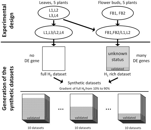
Generation of the synthetic data sets. To construct synthetic data sets, a full H0 data set containing no DE genes is generated by comparing biological replicates of leaves and a H1-rich data set containing a large proportion of DE genes is generated by comparing contrasted samples of leaves and flower buds. The synthetic data sets are generated by the random combination of the full H0 and H1-rich data sets. The control of the number of genes of the full H0 data set included in a synthetic data set allows modulating the proportion of NDE genes coming from both the full H0 and the H1-rich data sets. The subset of genes from the H1-rich data set, which has been validated by qRT-PCR, is included in all the synthetic data sets to evaluate the sensitivity of each method. For each scenario, 10 synthetic data sets are generated.
Definition of the sets of truly DE genes and truly NDE genes
For the estimation of the TPR, AUC and FDR, it is necessary to identify the true DE and NDE genes. However, as the synthetic data sets are not simulated but generated from real data sets, the exhaustive identification of the true DE genes and NDE genes is not possible. Nevertheless, the TPR can be estimated from a subset of DE genes. As qRT-PCR is often used as a gold standard for gene expression, the 251 DE genes previously identified by qRT-PCR among 333 randomly chosen genes were defined as the set of truly DE genes (DE set).
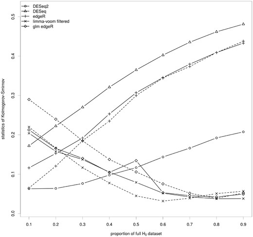
Impact of the key ingredients of the differential analysis on the calculation of the raw P-values. The median of the Kolmogorov–Smirnov test statistics for the set of methods covering the various parameters of the differential analysis of RNA-seq data are shown for synthetic data sets containing 10 (0.1) to 90% (0.9) of genes from the full H0 data set. These data sets contain many (0.1) to few (0.9) DE genes. The full lines correspond to methods without a filtering step and the dashed lines to the same methods with a filtering step. Results for each synthetic data set are shown in Figure S2.
Importantly, this correction of raw P-values is applied only for the identification of the truly NDE, but not when evaluating the performance of the nine methods.
The genes with a corrected raw P-value >0.05 were declared as truly NDE. We identified two sets of truly NDE genes for each synthetic data set. The first one consists of the genes coming from the full H0 data set plus those declared truly NDE by at least one of the five unfiltered methods. We refer to this first set as NDE.union, which may include some genes that are not truly NDE. The second solution is to consider genes declared truly NDE by all the five aforementioned methods. We refer to this second set as NDE.inter, which may exclude some truly NDE genes.
We consider both of these sets for the AUC and FDR evaluations. The genes that were not identified as truly DE or truly NDE were not taken into account for the estimation of the performances.
Data deposition and accession code
RNA-seq and microarray data were both deposited at Gene Expression Omnibus (http://www.ncbi.nlm.nih.gov/geo/, accession no. GSE45345 and GSE53673) and at CATdb (http://urgv.evry.inra.fr/CATdb/; Project: CAT-seq) according to the ‘minimum information about a microarray experiment’ standards [38]. The scripts, the real and synthetic data sets and their analysis are available from: http://ftp://urgv.evry.inra.fr/CATdb/Key_Ingredients_Differential_Analysis_RNAseq and https://github.com/mlmagniette/Key_ingredients_Differential_Analysis_RNAseq
Results
Relevance of the real and synthetic data sets
We generated diagnosis graphs including Principal Component Analysis (PCA), density plot and correlation plot (available in the ‘real_datasets’ folder) to assess the quality of the real data sets. The first axis of the PCA (48.79% of the variability) discriminates tissues, whereas the second (30.34% of the variability) discriminates tissues and sequencing machine. The density and correlation plots reflect the experimental design.
Comparing the transcriptome of Ls and FBs is expected to yield a large proportion of DE genes, and this hypothesis was supported by analyses using three different technologies (RNA-seq, microarray and qRT-PCR). The CATMAv6 microarray analysis identified 16 226 (43%) DE genes of 38 365 genes, and an extensive qRT-PCR validation on 333 randomly selected genes identified 251 DE genes, with a balanced composition between the up- and downregulated genes (Table S2). Differential analysis of the RNA-seq data was identified from 7898 (28%) to 13 627 (48%) DE genes of 28 106 studied mRNAs.
To ensure that the L samples are suitable to define the full H0 data set, we performed a differential analysis with all the considered methods. By definition, the biological coefficient variation (BCV) of the full H0 data set represents the coefficient of variation that would remain between biological replicates if sequencing depth could be increased indefinitely [12]. It is unusual but identical to the BCV of the H1-rich data set, showing that it is not because of the difference of sequencing machine. With a FDR controlled at 5%, 17 genes were declared differentially expressed by at least one method and were definitively excluded. Hence, the synthetic data sets are composed of 33 585 genes.
Using this full H0 data set allows a first evaluation of the methods. First, the KS test was rejected for the nine methods (P-value = 0), showing that the raw P-values are not properly estimated by any of the methods. Second, the type I error rate at a nominal significance threshold of 5% was calculated. It showed that DESeq has the lowest type I error rate (0.02%) followed by edgeR (0.09%), edgeR filtered (0.12%), DESeq2 (filtered or not) (2.40%), limma-voom (3.28%), limma-voom filtered (4.68%), glm edgeR filtered (4.94%) and glm edgeR (5.49%). As opposed to the results of Reeb and Steibel [26], all methods except glm edgeR produce less false positives than expected.
Similar diagnosis plots are provided in the sub-folder of each synthetic data set: library size, density plot of the raw counts, PCA and distribution of the H0 and truly DE genes. The density plots and PCA change progressively as expected with the proportion of full H0 data set. Mixing randomly the two data sets does not alter the library sizes or the distribution of the H0 and truly DE genes. The BCV of the synthetic data sets is similar to the BCV of the H1-rich data set.
Evaluation of the P-values
The varying number of genes from the full H0 data set in each synthetic data set influences the sensitivity of KS test. To compare all the synthetic data sets, this test is applied to 100 sets of 1000 random genes from the full H0 data set. In addition, we did not analyze DESeq2 with filtering because the filtering step occurs after the calculation of the raw P-values. Hence, the interpretation of the KS test in terms of fit of the model to the data is not relevant. After a Bonferroni correction, 69.34% of the KS tests were rejected at the 5% level. This result, based on random subsets of NDE genes, suggests that most of the time, the raw P-values are not properly calculated. A closer analysis of the KS test statistics shows two groups of methods (Figure 2). For DESeq and edgeR, filtered or not, the value of the statistic increased from 0.05 to 0.48 with the proportion of full H0 data set. DESeq2 is also part of this group but with lower values (0.05–0.21). On the contrary, for glm edgeR and limma-voom, filtered or not, it globally decreased from 0.30 to 0.03 with the proportion of full H0 data set. The slight increase of the value of the statistic for limma-voom around 50% of full H0 genes corresponds to variability across the 10 synthetic data sets (Supplementary Figure S2). Filtering stabilizes limma-voom. This result suggests that a generalized linear model or a linear model after data transformation, which allows accounting for the factors impacting the count distribution, improves the calculation of the P-values especially when the proportion of DE genes is not high. On the contrary, filtering does not improve the results except for limma-voom, where it stabilizes it for some scenarios.
The analysis of the distribution of the raw P-values of the NDE genes is relevant to estimate the fit between the model and the data set, but the usual criteria to evaluate the performances of differential analysis pipelines are the TPR, the FDR and the AUC.
Discrimination of DE and NDE genes
To construct the ROC curves, we used the DE set and both the NDE.inter set (Figure 3) and NDE.union set (Supplementary Figure S3). Both analyses show similar results, and there is no variability across the 10 synthetic data sets for any scenario or method. Regardless of the proportion of the full H0 data set, data filtering was found to slightly improve the AUC. For methods based on a linear model or its generalized extension for negative binomial distribution, the AUC was high and independent of the proportion of full H0 data set except for DESeq2 at 90% of full H0 genes. On the contrary, the AUC of the methods based on a simple negative binomial distribution steadily decreased with the increase of the proportion of full H0 data set when it is >0.3–0.4.
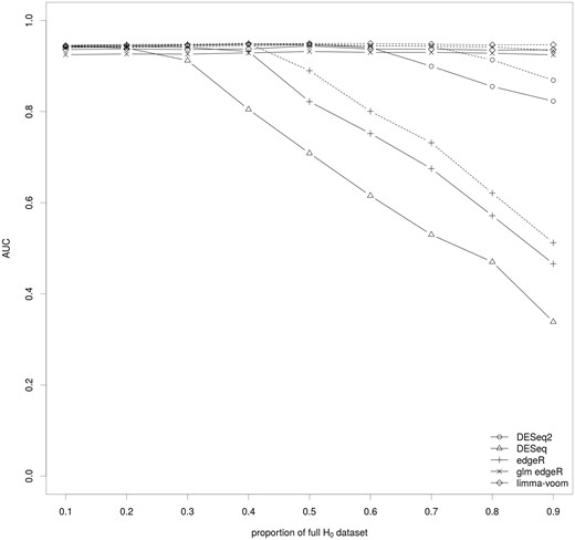
Impact of the key ingredients of the differential analysis on the AUC. The median of the AUC for the set of methods covering the various parameters of the differential analysis of RNA-seq data are shown for various proportions of genes of the full H0 dataset. The AUC were calculated using NDE.inter. The full lines correspond to methods without a filtering step and the dashed lines to the same methods with a filtering step.
Although AUC is a good measure at a global level, in practice, methods generate a list of differentially expressed genes based on a threshold on the adjusted P-values. This threshold must guarantee a control of the FDR. The following results are presented for a control of the FDR at the 5% level, meaning that genes are declared differentially expressed when their adjusted P-value is <0.05.
Control of the FDR
The FDR is defined as the proportion of truly NDE genes among the list of genes declared as differentially expressed. We note that, given the design of NDE.inter and NDE.union, the use of both presumably provides an approximate lower and upper bound of the FDR, respectively (Figure 4).
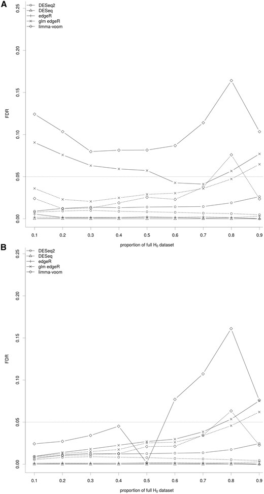
Impact of the key ingredients of the differential analysis on the FDR. The median of the FDR for the set of methods covering the various parameters of the differential analysis of RNA-seq data are shown for various proportions of genes of the full H0 data set. The full lines correspond to methods without a filtering step and the dashed lines to the same methods with a filtering step. (A) FDR calculated using NDE.union (upper bound). (B) FDR calculated using NDE.inter (lower bound). Values for each synthetic data set are shown in Figures S4 and S5, respectively.
As the tests were performed at a nominal 5% level, the FDR for all methods should be constant at 5%. However, the lower and upper bounds of most methods did not include this value. For the methods based on simple negative binomial distribution, the lower and upper bounds were close to 0, suggesting that they were conservative. For DESeq2, the FDR was higher and slightly increased with the proportion of full H0 data set, but was always lower than the nominal value. For glm edgeR, the interval defined by the upper and lower bounds generally contained the nominal value, suggesting that glm edgeR controlled the FDR correctly. For limma-voom, the FDR control seemed to be more variable, and it was associated with the variability across the 10 synthetic data sets for some scenarios, as already observed (Supplementary Figures S4 and S5). Nevertheless, the results suggest that limma-voom controlled the FDR correctly for data sets with a large number of DE genes. Finally, the filtered methods had a lower FDR than the corresponding unfiltered methods. Moreover, for limma-voom, the filtering step stabilized the behavior of the FDR.
Evaluation of the TPR
By definition, TPR is the proportion of truly DE genes correctly declared as differentially expressed. To evaluate it for each synthetic data set, the DE set was considered (Figure 5).
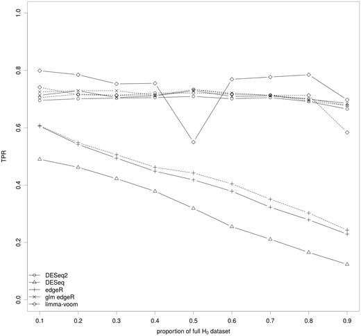
Impact of the key ingredients of the differential analysis on the TPR. The median of the TPR for the set of methods covering the various parameters of the differential analysis of RNA-seq data are shown for various proportions of genes of the full H0 data set. The full lines correspond to methods without a filtering step and the dashed lines to the same methods with a filtering step. Results for each synthetic data set are shown in Figure S6.
The TPR distinguished two groups of methods: methods using linear modeling after data transformation or glm modeling, and the others regardless of whether data were filtered. For the second group (DESeq and edgeR), we observed that the TPR was a function of the full H0 data set proportion. When this proportion increased (implying a smaller proportion of DE genes), the TPR decreased from 60 to ≤20%. We also observed that the filtering step did not change the TPR. DESeq2, glm edgeR and limma-voom had a high TPR independent of the full H0 data set proportion. The slight dip observed for limma-voom was once again associated to the variability across the 10 synthetic data sets for some scenarios (Supplementary Figure S6). Apart from stabilizing limma-voom, the use of data filtering seemed to have only a limited impact.
As the TPR of the methods is probably related to their FDR control, we calculated the TPR for an effective FDR of 5% using the DE set and the NDE.inter (Figure 6) or the NDE.union (Supplementary Figure S7) sets. Both analyses showed similar results, and there was no variability across the 10 synthetic data sets for any scenario or method. As expected, the TPR was improved and the graph is similar to the AUC graph (Figure 3): methods based on a linear model or its generalized extension for negative binomial distribution showed a constant and high TPR, whereas the methods based on a simple negative binomial distribution showed a steady decrease of the TPR, with the increase of the proportion of full H0 data set when it was >0.4–0.5.
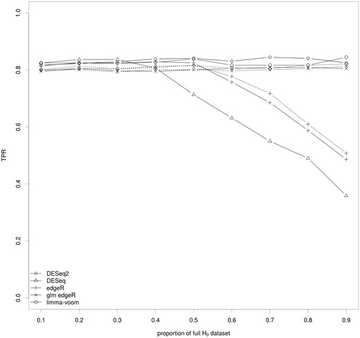
Impact of the key ingredients of the differential analysis on the TPR for a fixed FDR. The median of the TPR for an effective FDR at level 5% is calculated for the set of methods covering the various parameters of the differential analysis of RNA-seq data and for various proportions of genes of the full H0 data set using the NDE.inter set. The full lines correspond to methods without a filtering step and the dashed lines to the same methods with a filtering step.
Discussion
As simulated data sets are drawn from a given probability distribution, they allow the precise measurement of various statistical indicators because DE and NDE genes are known by design. However, for the same reason, these simulations are an approximation of reality. Furthermore, these probability distributions are often based on the statistical model and assumptions of particular analysis methods and hence can intrinsically favor those methods. A second option is to consider a large number of replicates and assume that the statistical methods are then identifying the true DE and NDE genes to then evaluate method performances for a smaller number of replicates [27]. On the contrary, synthetic data sets are not based on explicit assumptions on the underlying distribution and are generated by shuffling real data sets while still allowing the modulation of the proportion of NDE genes. The synthetic data sets share the same characteristics as the real data sets used to generate them. In addition, their creation can easily be automated and performed in a matter of seconds. However, synthetic data sets are more difficult to generate than simulated data sets because it is necessary to produce real data including several biological replicates and extensive external validations. Despite the large number of real data sets now available, sometimes with numerous biological replicates, the lack of extensive external validation prevents their use to generate synthetic data sets especially if AUC and TPR are estimated. In addition, it is not possible to exhaustively identify all DE genes and NDE genes. In this work, with few biological replicates, a representative subset of DE genes is identified through qRT-PCR on a random set of genes with both high and low expression levels, small or large log ratios. As it is always used to validate RNA-seq results, it can be seen as a golden standard but with some limitations. First, the differential analysis of qRT-PCR is not powerful because of the lack of replicates and the small number of tested genes. Also, despite a good concordance between the qRT-PCR and RNA-seq quantifications (R2 = 0.82 in this work), there are always some discrepancies, and it may explain why the TPR never reached values >85% in this study. The identification of the NDE genes is more difficult but critical for the estimation of the performances [25, 26]. One option is to consider only the genes from the full H0 data set, but then, the NDE set misses all the NDE genes coming from the H1-rich data set, which leads to a probable underestimation of the false positives. In this work, we identified the NDE genes coming from the H1-rich data set as the genes that are not declared differentially expressed by the methods. To be as accurate as possible and identify the true NDE genes as opposed to the declared NDE genes, we corrected the raw P-values for the identification of the NDE set (and only for this) and considered the union of all the NDE genes identified by the unfiltered methods tested in this study. This so-called NDE.union set may contain some truly DE genes and therefore it probably gives an upper bound of false positives. Similarly, considering NDE genes identified by all the tested methods (NDE.inter) probably gives a lower bound of false positives.
So, this resampling approach only allows bounds of statistical indicators to be calculated, but it does not favor a particular statistical model and allows a more realistic evaluation of statistical methods.
Using our benchmark approach, we explored the impact of (1) filtering genes, (2) the count distribution, (3) accounting for all covariates of the design in the definition of the mean and (4) the approach to estimate the variance on the performances of the differential analysis in scenarios with varying proportions of DE genes and two biological replicates. A recent study by Schurch et al. [27] explored complementary scenarios with varying number of replicates for a fixed proportion of DE genes. Interestingly, when comparing our most similar scenarios (synthetic data sets with 10% of full H0 genes versus their scenario with two to three replicates and T > 0.5), the observed TPR and FDR are similar. So, despite different data sets and definitions of DE and NDE genes, the results are consistent and probably allow a generalization of the results of these two studies.
Our results strongly suggest that writing the expectation of gene expression as a function of the factors of the experimental design has the highest impact on the final results. Once data are properly modeled, our results suggest that the filtering step is important to control the FDR. On the contrary, the impact of the specific approach to estimate the variance is limited. These results can be analyzed from two different perspectives: a practical and a statistical one.
From a statistical point of view, accounting for all covariates in the design improves significantly the performances of the methods. The distribution of the raw P-values from the H0 genes is closer to the expected uniform distribution; the AUC and TPR are maximal and stable across the tested scenarios, and the FDR is closer to the nominal value. We think that, when the mean of the expression is properly decomposed, the variance only captures the biological and technical variability, and the statistical model fits data better. Our results show that even in a simple comparison between two conditions with a small number of biological replicates, it is important especially in plant experiments where the harvest date should always be considered. This observation was not possible in the important evaluation performed by Soneson and Delorenzi [16] because of the evaluation framework based on simulation. Similarly, Schurch et al. do not find differences between methods based on simple negative binomial distributions and methods based on a linear model or its generalized extension for negative binomial distribution because their experimental design includes only one covariate. They observed a different behavior of glm edgeR compared with edgeR, which is unexpected in their design. We suspect that this difference comes from the different normalization procedure used for each method (upperquartile and TMM, respectively).
The count distribution and the approach to estimate the variance with a small number of replicates become less critical when the expectation of the count distribution takes all the information of the experimental design into account. Globally, DESeq2, glm edgeR and limma-voom performed similarly well. Nevertheless, when the proportion of DE genes is low, the behavior of DESeq2 in terms of raw P-value estimation, AUC and FDR control differs from glm edgeR and limma-voom. We found no obvious explanation to this behavior. When unfiltered, limma-voom shows some instability of the statistical indicators across the 10 synthetic data sets generated for 40, 50, 60 or 90% of full H0 data set. This instability is most probably owing to genes with low counts because filtering them out almost completely abolishes it. This result is similar to Schurch et al. [27] but opposed to Soneson and Delorenzi [16].
The filtering step also slightly improves the performances of the methods in terms of AUC and TPR. It also stabilizes the control of the FDR as already observed [16]. However, strictly speaking from a statistical point of view, it worsens it because the FDR values are more different from the expected 5% than for the values of the corresponding unfiltered methods. Nevertheless, from a practical point of view, a way to decrease the number of false positives while maintaining a high TPR is always desirable. Despite the drawback of removing a number of genes from the analysis, the filtering step provides this result. Combined with the inclusion of all covariates of the design through a linear model or its generalized extension for negative binomial distribution, it also stabilizes the performances of the methods, which probably means that they will be more robust for a large variety of data sets.
Estimating the performances of the methods on real data sets is critical. It is difficult even with benchmarks and the results do not systematically apply to particular data sets [16, 26, 27]. We showed that the performances of the methods considered here seem to be related to the accuracy of P-value calculation. Because the distribution of raw P-values is theoretically dominated by a uniform distribution, the accuracy of their calculation can be observed on the histogram of raw P-values. When the filtering step occurs after the calculation of the P-values (i.e. DESeq2), this property stands only for unfiltered raw P-values. This criterion was already used [6, 29, 30, 39] and therefore we propose to generalize its visualization as an additional quality control, which can be used for any real data set.
We propose a realistic framework to assess the impact of the key components of the statistical framework for differential analyses of RNA-seq data.
We recommend the inclusion of all relevant experimental factors in the mean decomposition by using linear or generalized linear models.
We recommend the visualization of the raw P-value histogram as another quality control criterion.
Supplementary Data
Supplementary data are available online at http://bib.oxfordjournals.org/.
Guillem Rigaill is an Assistant Professor of statistics at the University of Évry val d'Essonne, working at the Institute of Plant Sciences Paris Saclay IPS2 which is part of CNRS, INRA, Université Paris-Sud, Université Evry, Paris Diderot, Sorbonne Paris-Cité and Université Paris-Saclay.
Sandrine Balzergue is an engineer in plant biology formerly managing the transcriptomic platform of the Institute of Plant Sciences Paris Saclay IPS2 which is part of CNRS, INRA, Université Paris-Sud, Université Evry, Paris Diderot, Sorbonne Paris-Cité and Université Paris-Saclay. She is now working at INRA, UMR1345 Institut de Recherche en Horticulture et Semences, 49071, Beaucouzé, France.
Véronique Brunaud is an engineer in plant bioinformatics working at the Institute of Plant Sciences Paris Saclay IPS2 which is part of CNRS, INRA, Université Paris-Sud, Université Evry, Paris Diderot, Sorbonne Paris-Cité and Université Paris-Saclay.
Eddy Blondet is an engineer in plant biology formerly working at the Institute of Plant Sciences Paris Saclay IPS2 which is part of CNRS, INRA, Université Paris-Sud, Université Evry, Paris Diderot, Sorbonne Paris-Cité and Université Paris-Saclay. He is now working at Biotransfer, Paris, France.
Andrea Rau is a researcher in statistics working at GABI, INRA, AgroParisTech, Université Paris-Saclay, 78350 Jouy-en-Josas, France.
Odile Rogier is an engineer in plant bioinformatics formerly working at the Institute of Plant Sciences Paris Saclay IPS2 which is part of CNRS, INRA, Université Paris-Sud, Université Evry, Paris Diderot, Sorbonne Paris-Cité and Université Paris-Saclay. She is now working at INRA, UR0588 AGPF, 2163 Avenue de la Pomme de Pin, CS 40001 Ardon, F-45075 Orléans Cedex 2, France.
José Caius is a technician in plant biology working at the Institute of Plant Sciences Paris Saclay IPS2 which is part of CNRS, INRA, Université Paris-Sud, Université Evry, Paris Diderot, Sorbonne Paris-Cité and Université Paris-Saclay.
Cathy Maugis-Rabusseau is an Assistant Professor of statistics at the Institut de Mathématiques de Toulouse, INSA de Toulouse, Université de Toulouse, 31400 Toulouse, France.
Ludivine Soubigou-Taconnat is an assistant engineer in plant biology. She manages the transcriptomic platform of the Institute of Plant Sciences Paris Saclay IPS2 which is part of CNRS, INRA, Université Paris-Sud, Université Evry, Paris Diderot, Sorbonne Paris-Cité and Université Paris-Saclay.
Sébastien Aubourg is a researcher in Bioinformatics formerly working at the Institute of Plant Sciences Paris Saclay IPS2 which is part of CNRS, INRA, Université Paris-Sud, Université Evry, Paris Diderot, Sorbonne Paris-Cité and Université Paris-Saclay. He is now working at INRA, UMR1345 Institut de Recherche en Horticulture et Semences, 49071, Beaucouzé, France.
Claire Lurin is a researcher in plant biology working at the Institute of Plant Sciences Paris Saclay IPS2 which is part of CNRS, INRA, Université Paris-Sud, Université Evry, Paris Diderot, Sorbonne Paris-Cité and Université Paris-Saclay.
Marie-Laure Martin-Magniette is researcher in statistics working at Institute of Plant Sciences Paris Saclay IPS2 which is part of CNRS, INRA, Université Paris-Sud, Université Evry, Paris Diderot, Sorbonne Paris-Cité and Université Paris-Saclay. She is also part of the UMR MIA-Paris, AgroParisTech, INRA, Université Paris-Saclay, 75005, Paris, France.
Etienne Delannoy is a researcher in plant biology working at the Institute of Plant Sciences Paris Saclay IPS2 which is part of CNRS, INRA, Université Paris-Sud, Université Evry, Paris Diderot, Sorbonne Paris-Cité and Université Paris-Saclay.
Acknowledgments
The authors thank INRA-EPGV team and IG-CNS institute for Illumina library sequencing work.
Funding
The French Agence Nationale de la Recherche (ANR-13-JS01-0001-01, project MixStatSeq); the French Institut National de la Recherche Agronomique AIP bioressource 2010 project; the GIS Infrastructures en Biologie Santé et Agronomie AO Platform 2010 call. The IPS2 benefits from the support of the LabEx Saclay Plant Sciences-SPS (ANR-10-LABX-0040-SPS).
