


Abstract
Bacterial effector proteins secreted by various protein secretion systems play crucial roles in host–pathogen interactions. In this context, computational tools capable of accurately predicting effector proteins of the various types of bacterial secretion systems are highly desirable. Existing computational approaches use different machine learning (ML) techniques and heterogeneous features derived from protein sequences and/or structural information. These predictors differ not only in terms of the used ML methods but also with respect to the used curated data sets, the features selection and their prediction performance. Here, we provide a comprehensive survey and benchmarking of currently available tools for the prediction of effector proteins of bacterial types III, IV and VI secretion systems (T3SS, T4SS and T6SS, respectively). We review core algorithms, feature selection techniques, tool availability and applicability and evaluate the prediction performance based on carefully curated independent test data sets. In an effort to improve predictive performance, we constructed three ensemble models based on ML algorithms by integrating the output of all individual predictors reviewed. Our benchmarks demonstrate that these ensemble models outperform all the reviewed tools for the prediction of effector proteins of T3SS and T4SS. The webserver of the proposed ensemble methods for T3SS and T4SS effector protein prediction is freely available at http://tbooster.erc.monash.edu/index.jsp. We anticipate that this survey will serve as a useful guide for interested users and that the new ensemble predictors will stimulate research into host–pathogen relationships and inspiration for the development of new bioinformatics tools for predicting effector proteins of T3SS, T4SS and T6SS.
Introduction
Bacteria can form mutualistic or pathogenic associations with hosts such as humans through the regulation of their specialized protein secretion systems [1–3]. The process of protein secretion by bacteria requires induction of protein synthesis and then protein translocation from the bacterial cytoplasm into host cells [4]. A secreted protein may either remain associated with the outer membrane, or be injected into eukaryotic (host) cells or into neighbouring bacterial cells [5]. To date, nine distinct types of protein secretion systems have been experimentally characterized in gram-negative bacteria [2, 3, 6–10], which are referred to as type I to type IX. Various enzymes are exported to the environment by the type I, type II or type V secretion systems [5]. In contrast, type III secretion system (T3SS), type IV secretion system (T4SS) and type VI secretion system (T6SS) [11–18] transport ‘effector’ proteins into host cells. By definition, effector proteins mimic the function of host proteins and can thereby dysregulate host cell biology to the benefit of the bacterium. Effector proteins secreted by the T3SS, T4SS and T6SS are, respectively, named T3SE, T4SE and T6SE. The numbers of experimentally validated effectors vary across bacterial species, with respect to different hosts and according to various survival strategies [11, 19, 20].
In light of the biological significance of bacterial effector proteins, a number of computational approaches were developed to predict secreted effector proteins based on protein-sequence information [21–23]. An important consensus from previous studies was that simplified statistical methods based on individual features alone, such as sequence similarity, sequence patterns and gene-adjacent sequence features, did not perform well for effector protein prediction [24–26]. Therefore, since 2009, machine learning algorithms have been increasingly used to address this difficult task by formulating effector protein prediction as a classification problem. The machine learning algorithms used to date include support vector machines (SVMs) [19, 27–32], artificial neural networks (ANNs) [27], Markov or hidden Markov models [33], Naïve Bayes [34] and Random Forest (RF) [4]. Among these machine learning techniques, SVMs are the most widely used algorithms for prediction of effector proteins. A variety of features, such as compositions of amino acids and amino acid pairs, position-specific scoring matrices (PSSMs), physicochemical properties and protein secondary structures (SS), were commonly extracted and used as an input to train the machine learning models. Cross-validation tests including leave-one-out and k-fold cross-validation are widely applied to assess the performance of the developed methods.
The currently available methods for secretion effector prediction differ significantly from one another in terms of learning algorithms, data sets (divided into training and test data sets), features used, prediction performance, availability via designated web servers and/or stand-alone software and applicability. In this article, we aim to provide a comprehensive survey and performance evaluation of currently available methods and tools for the prediction of three major types of secretion effector proteins, namely, T3SEs, T4SEs and T6SEs. To the best of our knowledge, this is the first in-depth comparison of its kind. It is particularly notable that, while there have been a number of machine learning-based methods for the prediction of T3SEs and T4SEs, little work has been done for prediction of the effectors of the more recently discovered T6SS [35, 36]. Experimental studies have proposed several motifs for identifying T6SEs [37, 38], and here we evaluate the performance of motif pattern-based approaches for predicting T6SEs by using the independent test data set extracted from the previous studies of Salomon et al. and Altindis et al. [37, 38].
Based on the performance evaluation of current methods for effector protein prediction, we developed three ensemble classifiers by integrating the output of all reviewed methods in this study. Three machine learning algorithms, i.e. SVM [39], RF [40] and Logistic Regression (LR) [41, 42], were used to train the ensemble classifiers. The three classifiers took the output of all individual predictors as input. The performance was then evaluated using 5-fold cross-validation. Our results indicated that the three ensemble models outperformed all individual tools for both T3SEs and T4SEs. We anticipate that these ensemble models will complement existing methods and provide new insights into the roles of secreted effectors of T3SS and T4SS.
Materials and methods
Construction of the independent test data sets
We searched through several publicly available databases to extract data associated with T3SE, T4SE and T6SE and construct the independent test data sets. Figure 1 depicts the flowchart of our data-curation procedures for the creation of independent test data sets.
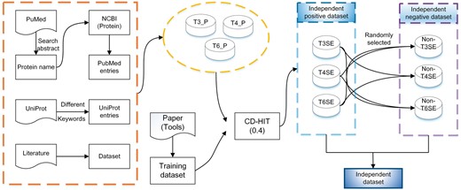
Flowchart of the independent test data set collection for T3SEs, T4SEs and T6SEs.
Initially, we searched through the UniProt database [43] using various keywords describing different types of bacterial secreted effector proteins. Such keywords included ‘effector protein’, ‘bacterial secretion effector’ and ‘translocated into the host cell’ and were used in combination with ‘type III secretion system’ (‘T3SS’), ‘type IV secretion system’ (‘T4SS’) or ‘type VI secretion system’ (‘T6SS’), or their associated effector acronyms ‘T3SE’, ‘T4SE’ and ‘T6SE’, respectively. This search strategy resulted in a large number of redundant entries for the same effectors. These were then manually checked and filtered to ensure the quality of extracted entries. Subsequently, proteins that did not genuinely belong as T3SE, T4SE or T6SE were removed. All retained entries were required to have unambiguous and explicit annotations, as well as evidence for their classification (in form of statement such as ‘secreted by T3SS’, or ‘translocated into the host cell via the type IV secretion system’).
Secondly, a number of additional effector proteins were collected from curated data sets in previous studies. Although many of these proteins can be found in the NCBI protein database (http://www.ncbi.nlm.nih.gov/protein/), they are not necessarily annotated as such. For example, only the 100 N-terminal amino acids of non-redundant T3SEs are used in BPBAac [32] (with three information factors for each entry, including gene name, bacteria species and PMID number provided). This information was then used to extract full protein sequence entries from NCBI; full-length protein-sequence information is mandatory for our study, as the complete N- and C-terminal residue information is required for feature extraction and calculation. Wherever necessary, we extracted the complete amino acid sequences of these entries by searching their corresponding protein names provided in the literature.
Thirdly, we mined the relevant literature by searching the abstract in PubMed to obtain the most recent secreted effector proteins not currently included in public sequence databases. We then used their protein and/or gene names to search in the NCBI protein database to validate and retrieve their sequences in FASTA format.
After these steps, all extracted effector proteins of T3SS, T4SS and T6SS constituted the positive data sets, which are referred to as T3_P, T4_P and T6_P, respectively. As a final procedure, to objectively evaluate and compare the performance of all reviewed methods/tools, we downloaded, whenever possible, the original training data sets used for developing these approaches and removed all the duplicate proteins from T3_P, T4_P and T6_P. To generate the negative data sets of non-effectors for each of the bacterial secretion systems, we randomly selected proteins from the positive data sets representing the other two secretion systems. For example, when constructing the negative data set for T3SS, we randomly chose effector proteins from the independent test data sets for T4SS and T6SS. Similar to the construction procedure for positive data sets, we removed all duplicate non-effector sequences from the negative data sets for all three secretion systems.
To avoid potential overestimation of the prediction performance, the CD-HIT program (available at http://weizhong-lab.ucsd.edu/cd-hit/) was used to remove sequence redundancy from both positive and negative data sets for the three secretion systems. CD-HIT is a widely used bioinformatics tool for clustering protein sequences according to a specified sequence identity threshold, which was set at 40% for this study [44]. As a result, 44 T3SEs, 40 T4SEs and 237 T6SEs were retained following removal of sequence redundancy. We randomly selected the same numbers of negative samples based on CD-HIT clustered negative sequences for each secretion system. In summary, three independent test data sets were constructed, with each of these including effector proteins and non-effector proteins for each of the bacterial secretion systems, i.e. III (44 T3SEs versus 44 non-T3SEs), IV (40 T4SEs versus 40 non-T4SEs) and VI (237 T6SEs versus 237 non-T6SEs), respectively.
To explore potential amino acid enrichment or depletion in either N- or C-terminal residue positions for secreted effector proteins, sequence-logo representations were generated for the 50 N-terminal and 50 C-terminal residue positions based on the curated data sets by using pLogo [45]. pLogo is a probabilistic approach for the identification and visualization of sequence motifs, and was used for this analysis. The background data set for this motif-visualization analysis included the protein sequences obtained by searching the UniProt database.
Existing approaches for effector protein prediction
Tables 1 and 2 summarize the currently available prediction methods/tools for T3SEs and T4SEs, respectively. Notably, for T3SE predictors, SVMs were adopted as the predominant machine learning algorithm by multiple tools, including ANN [27], SIEVE [31], BEAN [28], BEAN 2.0 [29] and BPBAac [30]. Apart from SVMs, several methods used other machine learning algorithms, including RF model [4], EffectiveT3 [34], T3SEdb [46] and T3_MM [33]. As to T4SE predictors, we evaluated two currently available tools, namely, T4EffPred [19] and T4SEpre [32], as T4SE predictors. For T6SE predictors, there are no other tools currently available aside from motif-based search methods. Therefore, to evaluate the performance of T6SE prediction, we used specific motifs previously proposed, including MIX (marker for type six effectors) [37] and the motifs from Altindis et al. [38]. These approaches will be described in detail in subsequent sections.
A Comprehensive list of the reviewed methods/tools for the prediction of T3SEs for the bacterial type III secretion system
| Toola (year) | Software availability | Webserver availability | Feature representation | Algorithm | Performance evaluation strategy | Training data set | Test data set | Reference | |
|---|---|---|---|---|---|---|---|---|---|
| #Effectors | #Non-effectors | ||||||||
| ANN (2009) | No | Yes | SEQ | ANN & SVM | 10-fold cross-validation (leave 50% out) | 575 | 685 | n/a | [24] |
| SIEVE (2009) | No | Yes | AAC; GC; PHYL; CON; SEQ | SVM | Independent test | n/a | n/a | n/a | [28] |
| EffectiveT3 (2009) | Yes | Yes | SS | Naïve Bayes | 10-fold cross-validation | 167 | n/a | [30] | |
| T3SEdb (2010) | No | Yes | Hydrophobicity; polarity; β-turns | Naïve Bayes | 10-fold cross-validation and independent test | 100 | 100 | Effectors: 68Non-effectors: 68 | [41] |
| T3_MM (2013) | Yes | Yes | AAC | Markov model | 5-fold cross-validation and independent test | 154 | 308 | 35 | [42] |
| RF model (2013) | Yes | No | AAC; SS; RSA; PP | RF model | 5-fold cross-validation and independent test | 191 | 213 | 121 | [4] |
| BEAN (2013) | Yes | No | HH-CKSAAP | SVM | 5-fold cross-validation and independent test | 154 | 308 | 323 | [25] |
| BEAN 2.0 (2013) | No | Yes | HH-CKSAAP | SVM | 5-fold cross-validation | 243 | 486 | n/a | [26] |
n/a, not applicable; RSA, relative solvent accessibility; PP, physicochemical properties; GC, G + C nucleotide compositions of the primary DNA sequence; PHYL, phylogenetic profile; CON, sequence conservation; SEQ, N-terminal sequence of protein; DPC, dipeptide composition; PSSM_AC, auto covariance transformation of PSSM.
The URL addresses for accessing the listed tools are provided as follows:
EffectiveT3—http://www.effectors.org/effective/submit.
T3_MM—http://biocomputer.bio.cuhk.edu.hk/softwares/T3_MM; http://biocomputer.bio.cuhk.edu.hk/T3DB/T3_MM.php.
BEAN 2.0—http://systbio.cau.edu.cn/bean/.
A Comprehensive list of the reviewed methods/tools for prediction of T4SEs of the bacterial type IV secretion systema
| Toolb (Year) | Software Availability | Webserver Availability | Feature representation | Algorithm | Performance Evaluation Strategy | Training data set | Test data set | Reference | |
|---|---|---|---|---|---|---|---|---|---|
| #Effectors | #Non-effectors | ||||||||
| T4EffPred (2013) | Yes | Yes | AAC; DPC; PSSM; PSSM_AC | SVM | Leave-one-out | 340 | 1132 | n/a | [19] |
| T4SEpre (2014) | Yes | No | AAC; SA; SS | SVM | 5-fold cross-validation | 347 | 694 | n/a | [29] |
Refer to the abbreviations in Table 1 for full descriptions of the feature representation and algorithms.
The URL addresses for accessing the listed tools are provided as follows:
T4EffPred—http://bioinfo.tmmu.edu.cn/T4EffPred.
Algorithms used by existing approaches
An SVM classifier is a powerful algorithm widely applied to solve many classification tasks in the field of computational biology [47–55]. It can be used to build linear or non-linear classification models by transforming input vectors into a high-dimensional space and constructing an optimal separation hyperplane between the positive and negative samples [56]. SVMs often achieve better or competitive performances compared with other machine learning techniques. Consequently, SVMs are also used for effector protein prediction of T3SEs [SIEVE, BPBAac, BEAN and BEAN 2.0 (Table 1)] and T4SEs [T4EffPred and T4SEpre (Table 2)].
The SIEVE model was the first SVM-based approach used to predict T3SEs [31] and was developed using the Gist software package [57], which is an online SVM classification software, based on both protein- and DNA-sequence information. The radial basis function was chosen as the core kernel of the SVM with a width of 0.5 and an optimized ratio of negative-to-positive examples to perform the classification [31].
BPBAac is also an SVM-based approach for predicting T3SEs that trains the prediction models based on amino acid composition (AAC) features extracted using the bi-profile Bayesian (BPB) feature-extraction scheme [58, 59]. The radial basis function K (si, sj) = exp (−γ‖si − sj ‖2) was selected as the core kernel of the SVM model. Its parameter γ and the penalty parameter C was then optimized via a grid search based on 10-fold cross-validation.
BEAN is a sophisticated approach used for identifying T3SEs and combines a hidden Markov model-based search method called HHbits with profile-based k-spaced AAC (CKSAAP) to extract the feature vector called HH-CKSAAP and train a linear kernel SVM model [28]. The SVM model was trained with the parameter cost C = 1 and tolerance of termination criterion e = 1 × 10⁻⁴. BEAN 2.0 is an advanced version of BEAN [29] that exploits more informative features for training the model on a larger data set as compared with BEAN.
T4EffPred is an SVM-based tool for predicting T4SEs and integrates the library for SVMs toolbox in the MATLAB workspace to build a prediction model based on different types of sequence-derived features, including AAC, dipeptide composition, PSSM and PSSM autocovariance transformation. Here, too, the SVM kernel is the radial basis function with parameters γ and C optimized using a grid search based on 10-fold cross-validation.
T4SEpre is yet another SVM-based tool for predicting T4SEs. It takes into account a number of different features and their combinations, including sequential AAC features, single-profile Bayesian (SPB) AAC features, BPB AAC features and joint position-specific features of AAC, SS and solvent accessibility (SA). The optimal parameters were the same as those used by T4EffPred.
Another popular machine learning technique is ANN, as it is able to deal with non-linear and high-dimensional data [60, 61]. The ANN tool was developed by combining both ANN (feed-forward-type architecture with a single hidden neuron layer) and SVM algorithms to train the optimal model using the signal sequence located within the first 30 amino acids at the N-terminus [27]. This method used a gradient-descent back-propagation learning scheme, with momentum at an adaptive learning rate. The output of the ANN was converted into a binary decision using a cut-off threshold value of θ = 0.5. For the SVM classifier, the complexity parameter C and the parameter γ of the radial basis function were optimized using a grid search in the logarithmic space.
A Markov model [62] has also been used for the prediction of secretion effector proteins. T3_MM adopted a straightforward Markov model based on the AAC of the 100 N-terminal amino acid residues to achieve a more stable classification performance [33]. Based on the Markov model, a sequential likelihood-ratio variable, R was created to measure the overall difference in the conditional probability profiles of position-adjacent AAC between T3SEs and non-T3SEs. The R-values were calculated and statistically analysed for T3SEs and non-T3SEs.
A Naïve Bayes classifier is a machine learning algorithm used mainly for solving supervised classification tasks and provides a simple approach by assuming that numeric attributes follow a single Gaussian distribution [63]. Given its attractive features, including its simple structure and ease of implementation, Naïve Bayes classifiers perform well in many real-world applications [64]. EffectiveT3 is a Naïve Bayes-based tool used for predicting T3SEs, by integrating a variety of N-terminal sequence features such as amino acid frequencies, short peptides and residues with certain physicochemical properties [34]. Notably, when using EffectiveT3 [34] to predict potential T3SEs, the choice of an appropriate probability threshold for the ‘secreted’ class (used to adjust the selectivity and sensitivity of the predictor) is set following user discretion. T3SEdb is another Naïve Bayesian classifier for T3SE prediction and was constructed using physico-chemical properties, such as hydrophobicity, polarity and β-turns, along with N-terminal motifs (100 amino acids). T3SEdb was implemented using WEKA [46], which is a well-established and widely used data-mining platform.
In recent years, RF emerged as a powerful machine learning algorithm and has been increasingly applied to solve many classification/regression problems [65–69]. It is especially efficient at dealing with data sets with high-dimensional features [45]. The ensemble of decision trees built by RF can reduce the bias of single decision trees, thereby improving overall prediction accuracy. The RF model developed by Yang et al. [4] predicts T3SEs and uses protein-sequence information, including AAC, SA, SS and six physicochemical properties, as well as the sequence fragment of 52 position-specific residues, to train the RF model [4]. The model has two parameters: ntree, the number of trees to build, and mtry, the number of variables randomly selected as candidates for each node. Both parameters are optimized using a grid-search approach. For this study, ntree took on values between 500 and 2500, in steps of 500, and mtry was set to integer values between 1 and 40. The RF algorithm was implemented using the RF package written in R [70].
Feature selection
The purpose of feature selection is to identify the most informative and contributive features to model performance and remove noisy and redundant features, to optimize prediction performance [71–73]. Given that initial features often contain noisy and redundant information, more studies use feature-selection techniques to characterize feature importance before the training of final optimized models. In this section, we briefly discuss the application of feature selection by different tools and summarize their results.
Among the reviewed tools, BPBAac, SIEVE, RF, Effective T3 and T3SEdb used feature-selection techniques to filter irrelevant features and characterize feature contributions to the performance of their methods. For the remaining predictors, it was unclear whether feature-selection strategies were used.
In SIEVE [31] the most important features were selected via an iterative process called recursive feature elimination. This process successively eliminates features exhibiting low impact on overall model performance. In comparison, RF adopted permutation importance analysis to facilitate optimal feature selection, resulting in 62 optimal features [4]. To identify the most informative features, EffectiveT3 used two feature-selection strategies provided by WEKA, including a greedy hill-climb search [74] (the BestFirst algorithm using a look-up-cache size of one and five iterations) and correlated feature selection [75] (locally predictive = true, missing values = false). For T3SEdb, a greedy stepwise algorithm [76] was used to select a reduced feature set consisting of individual physicochemical properties. After feature selection, 92 individual features, including hydrophobicity, polarity and β-turns, were reduced to 63 combined features. BPBAac adopted both the BPB and SPB method for feature extraction. The two methods are similar except that BPB also takes the features of negative-training data into consideration. Additionally, Löwer et al. found that the effector proteins of T3SS share common sequence-based features at the N-terminus (the 30 N-terminal residues). These sequence-based features were shown to contribute to accurate predictions of T3SEs [27].
Software functionality
In this section, we discuss the user-friendliness of graphical interfaces and functionalities of existing tools. Tools, such as BEAN 2.0, EffectiveT3 and ANN, enable users to submit multiple protein sequences in the FASTA format, although they have limitations regarding the maximum number of sequences allowed (for BEAN 2.0 and EffectiveT3, ≤200 protein sequences are permitted; for ANN, ≤50 protein sequences are allowed). However, T3_MM and T4Effpred only allow submissions of single-sequence queries in the FASTA format at a time, i.e. submission of multiple sequences is not allowed. Additionally, SIEVE is capable of predicting effector proteins by allowing users to upload files containing FASTA-formatted protein sequences. SIEVE and EffectiveT3 return the prediction outcome after the submission task is completed by sending an email to users instead of redirecting the output to a webpage. Depending on the task at hand, this might be a limitation, owing to the indirect retrieval of the prediction outcome.
Four tools, EffectiveT3, BPBAac, T3_MM and T4SEpre, also provide stand-alone software written in R, Perl and other programming languages to enable users to perform prediction analyses on local computers. Detailed instructions providing useful guidance and help for troubleshooting during installation and use are found on the corresponding websites. Furthermore, T4Effpred provides several different predictors implemented in MATLAB, based on different feature combinations and methods [19].
Additionally, detailed on-site help documents and examples of job submissions, if available, can facilitate the user understanding of prediction procedures and requirements. In this regard, BEAN 2.0, T3_MM and EffectiveT3 provide example sequences, allowing users to quickly get familiarized with the format of sequence submissions. Descriptions of sequence-length limitations, the maximum allowable number of sequences per submission, introduction of the prediction algorithms and methods and results interpretation are available for all tools. These various help documents provide useful information promoting users’ understanding of tool methodologies, requirements and limitations.
Performance evaluation measurements
Cross-validation (including k-fold cross-validation and leave-one-out cross-validation) and independent tests are often used to assess prediction performance. To perform k-fold cross-validation, the entire data set is divided into k subsets. Subsequently, at each cross-validation step, one subset constitutes the validation set, while the remaining k-1 subsets are combined to form the training data set. This procedure is repeated k times until all subsets have been used as both training and test sets. The average performance across all k trials is then computed and reported. Leave-one-out cross-validation can be regarded as an extreme case of k-fold cross-validation, with k = N, where N is the total number of samples in the data set. Similarly, each instance in the data set is used as a validation sample, whereas the remaining N − 1 samples are used to form the training data set and to train the prediction model. As a result, the average performance of the N models is reported as the final prediction performance of leave-one-out cross-validation. In contrast, the independent test provides a more objective performance evaluation. The independent test is conducted on a separate test data set by using a presumably different data distribution as compared with the training data set. To perform independent test cross-validation, it is necessary to ensure that there are no overlapping data points between the training data set and the independent test data set. An important consideration is that all sequence entries in the independent test data set have minimal sequence similarity with those included in the training data set.
The prediction performance of all the reviewed tools, except SIEVE, was evaluated by performing k-fold cross-validation tests in their original studies (i.e. 10-fold cross-validation for ANN and EffectiveT3, 5-fold cross-validation for T3_MM, RF, BEAN, BEAN 2.0 and T4SEpre, and leave-one-out cross-validation for BPBAac and T4EffPred). The performance of SIEVE, BPBAac, T3_MM and RF was also evaluated using independent tests in their original studies. Here, we comprehensively assessed the performance of all reviewed tools by performing tests based on independent data sets.
Results and discussion
Analysis of sequence motifs of known effector proteins
For each type of effector protein, N- and C-terminal sequences were extracted using a window size of 50 amino acids based on previous studies [19, 30]. The generated sequence logos for each type of effector protein are displayed in Figure 2.

Sequence-logo representations illustrating the amino acid preferences of both N- and C-terminal sequence motifs of the three different types of secreted effector proteins, (A) T3SEs, (B) T4SEs, (C) T6Ses and (D) the control (i.e. cytoplasmic proteins). Amino acids located above the X-axis are favourable, while those underneath the X-axis are unfavourable at the corresponding positions.
Ignoring the methionine at position 1, which is responsible for translation initiation, several notable preferences of amino acid residues are observed in Figure 2. While there is an overall lack of conservation in the C-terminal sequence, except for a preference for glutamine residues at position 4 and, to a lesser extent, at positions 1, 3, 6, 21, 32, 33 and 39 (Figure 2A), there is somewhat more striking conservation in the N-terminal region of the T3SE sequences. The N-terminal sequence motifs of T3SEs exhibit an enrichment with serine residues across multiple positions, including positions 6 to 10, 12, 13, 17, 18, 20, 21 and 31 to 34, and enrichment with isoleucine residues at positions 3 and 4, while leucine residues are depleted (Figure 2A). These observations are consistent with a number of experimental studies on individual T3SEs. For example, isoleucine residues contribute to the secretion of YopD, a T3SE of Yersinia pseudotuberculosis [78], and isoleucine and serine residues in YopE promote its secretion by the T3SS in Yersinia [79, 80]. Predictive analysis of residue preference in T3SE from Salmonella and Pseudomonas show prevalence of isoleucine and serine in the N-terminal region [79], and more broad analysis of T3SEs also highlight the over-representation of these amino acids in the N-region of T3SEs [30, 34].
In the case of T4SEs, several studies have suggested that C-terminal residues appear to provide the targeting information for protein translocation [81, 82]. Other recent studies showed that targeting information can be encoded in the N-terminal region of at least some T4SEs [83–85]. The sequence logos associated with the N- and C-terminal motifs of T4SEs are displayed in Figure 2B. In particular, we found that lysine and asparagine residues are favoured in the N-terminal sequences (Figure 2B). For C-terminal motifs, we observed a preponderance of glutamate at positions 35–41 and serine at positions 42–47 for the T4SEs. The enrichment with glutamate and serine is consistent with a previous computational study of T4SE proteins [32]. The motif analysis also makes clear that the final three positions at the C-terminus favour hydrophobic or positively charged residues, particularly asparagine, lysine and leucine. Experimental investigations of specific T4SEs in Legionella pneumophila and Agrobacterium tumefaciens have suggested that such hydrophobic or positively charged residues are essential for functional translocation signals that assist protein secretion [13, 81, 82], and the motif analysis presented here suggests this to be a general rule.
For T6SE N-terminal sequences, there was no striking conservation of residues that would suggest a targeting signal. At most, serine was frequently observed at position 2, and lysine was favoured at the final four positions at the C-terminus (Figure 2C). A previous case study of Hcp (haemolysin co-regulated protein) secretion by the T6SS of Edwardsiella tarda indicated that positively charged residues such as lysine are important for translocation by the T6SS [11, 86]. While this is consistent with positively charged residues close to the C-terminus contributing to a recognition sequence in T6SEs, this simple feature alone would not discriminate T6SEs from many other (non-secreted) proteins in the bacterial cytoplasm.
In terms of the N-terminal sequences of the control (i.e. cytoplasmic proteins), serine was favoured at position 2, while the enrichment of lysine and isoleucine at positions 3, 4 and 5, 6, 7 was also observed. For the C-terminal sequences of the control, we observed an overrepresentation of lysine residues at the final six positions 45–50.
Analysis of characteristic sequence lengths and amino acid frequencies for different types of effector proteins
By definition, effector proteins contain one or more domains that mimic functions important to host cell biology. As a result, variation in effector protein-sequence length reflects the diversity and/or complexity of their specific functional roles [87]. To elucidate the distribution of sequence lengths for T3SEs, T4SEs and T6SEs, we calculated their respective protein-sequence lengths (Figure 3). The resulting histograms showed that there are a large number of sequences with a similar length of 300–500 amino acid residues. The three classes of effector proteins exhibited similar sequence-length distributions, despite the fact that the T3SS, T4SS and T6SS protein translocase machinery is quite distinct in its architecture and therefore in the physical constraints that might be expected to be placed on the substrate (i.e. effector) proteins.
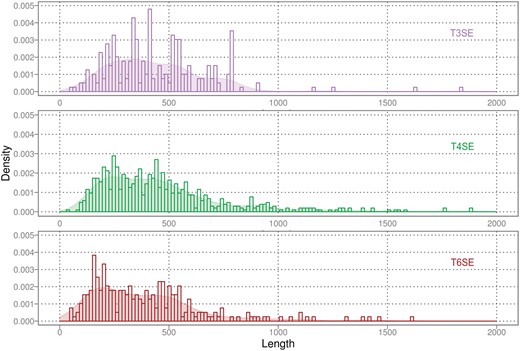
Distribution of sequence lengths for the complete sets of T3SEs, T4SEs and T6SEs.
Recently, it has been observed that overall AAC, as well as structural elements, tend to distinguish secreted proteins from cytoplasmic proteins [88]. Analysis of the AAC in T3SEs, T4SEs and T6SEs showed similarities in the frequency distributions between the three types of effector proteins (Figure 4). For example, leucine and serine were frequently found across the three classes of effector proteins. Leucine was identified as being important for protein binding and transport [89, 90] and, in at least one example, the effector protein SlrP secreted by the Salmonella T3SS has leucine-rich repeats with several conserved leucine residues present in a region shown to be important for translocation by the T3SS [91–93]. The three classes of effector proteins exhibited some specificities in regard to amino acid frequency, for example in that glutamate, alanine and lysine occurred more frequently in T4SEs than in T3SEs and T6SEs.
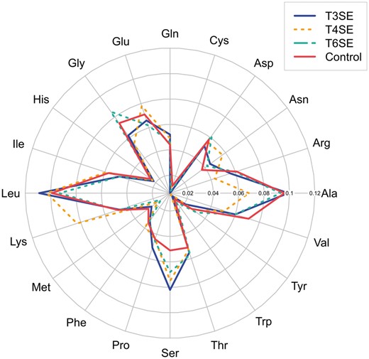
Variations in the frequencies of the 20 amino acids between T3SEs, T4SEs, T6SEs and the control (i.e. cytoplasmic proteins).
To address the significance of these perceived differences, statistical tests including the Mann–Whitney U-test and the permutation test on amino acid frequencies were conducted (Table 3). The Mann–Whitney U-test was performed using the default implementation in R [94], while the permutation test was executed through the R package DAAG [95]. The results of the Mann–Whitney U-test showed that the most differentially distributed amino acids between T3SEs and T4SEs were alanine, glutamate, phenylalanine, isoleucine, lysine and tyrosine. Serine and valine exhibited differential rates of occurrence between T3SEs and T6SEs, while the frequencies of alanine, glycine, lysine, asparagine and valine were significantly different between T4SE and T6SE. Notably, alanine and lysine occurred at significantly higher rates between T4SE and the other two classes (T3SE and T6SE), with valine present at significantly different levels between T6SE and the other two classes (T3SE and T4SE). Serine appeared to be the most significantly different amino acid type between T3SE/T4SE/T6SE and the control. In addition, glycine, asparagine and valine were also found to be significantly different between T3SE and the control, while between T6SE and the control arginine was significantly different. In contrast, the frequencies of alanine, phenylalanine, glycine and isoleucine were significantly different between T4SE and the control. Results from the permutation test indicated a differential preference for proline between T3SE and T4SE, while glycine and asparagine were significantly distributed between T3SE and T6SE, and serine occurred at significantly different percentages between T4SE and T6SE. Glutamine, threonine and isoleucine occurred with significantly different values of frequency between the control and three classes (T3SE, T4SE and T6SE), respectively.
Statistical analysis of residue frequencies in T3SEs, T4SEs, T6SEs and the control
| Residue | Mann–Whitney U-test | Permutation test | ||||||||||
|---|---|---|---|---|---|---|---|---|---|---|---|---|
| T3SE versus T4SE | T3SE versus T6SE | T4SE versus T6SE | T3SE versus control | T4SE versus control | T6SE versus control | T3SE versus T4SE | T3SE versus T6SE | T4SE versus T6SE | T3SE versus control | T4SE versus control | T6SE versus control | |
| Ala | < 2.2e-16 | 5.574e-06 | < 2.2e-16 | 0.5382 | <2.2e-16 | 1.065e-11 | 0 | 0 | 0 | 0.0218 | 0 | 0 |
| Cys | 0.01706 | 0.6646 | 0.04139 | 0.0006099 | 0.06653 | 0.001861 | 0.157 | 0.421 | 0.59 | 0.00255 | 0.0761 | 0.048 |
| Asp | 0.8355 | 0.181 | 0.1099 | 4.437e-06 | 5.298e-12 | 0.01268 | 0.908 | 0.308 | 0.211 | 2.2e-05 | 0 | 0.00323 |
| Glu | < 2.2e-16 | 0.05352 | 2.481e-12 | 1.634e-08 | 5.354e-16 | 0.007167 | 0 | 0.363 | 0 | 0 | 0 | 0.00033 |
| Phe | < 2.2e-16 | 9.65e-08 | 0.0002624 | 0.09596 | < 2.2e-16 | 3.224e-10 | 0 | 0 | 0.00202 | 0.137 | 0 | 0 |
| Gly | 1.334e-13 | 2.035e-06 | < 2.2e-16 | <2.2e-16 | < 2.2e-16 | 0.03622 | 0 | 2e-06 | 0 | 0 | 0 | 0.157 |
| His | 0.04773 | 0.01399 | 0.137 | 0.6091 | 0.01994 | 0.003644 | 0.028 | 0.0691 | 0.728 | 0.618 | 0.00677 | 0.0356 |
| Ile | < 2.2e-16 | 5.365e-08 | 0.0007238 | 1.032e-05 | < 2.2e-16 | 0.0001144 | 0 | 4e-06 | 0.017 | 0.00203 | 0 | 8e-06 |
| Lys | < 2.2e-16 | 0.2072 | < 2.2e-16 | 0.1926 | < 2.2e-16 | 0.0002296 | 0 | 0.18 | 0 | 0.805 | 0 | 0.0623 |
| Leu | 8.791e-07 | 0.3577 | 0.0006466 | 0.2076 | 2.253e-09 | 0.9158 | 2.8e-05 | 0.369 | 0.00368 | 0.472 | 0 | 0.634 |
| Met | 9.062e-11 | 0.7491 | 3.065e-10 | 0.06599 | < 2.2e-16 | 0.1951 | 0 | 0.542 | 0 | 0.0877 | 0 | 0.415 |
| Asn | 0.01269 | 7.135e-07 | < 2.2e-16 | < 2.2e-16 | < 2.2e-16 | 4.977e-12 | 0.000702 | 2e-06 | 0 | 0 | 0 | 0 |
| Pro | 1.278e-05 | 1.425e-05 | 0.2677 | 0.1533 | 1.411e-08 | 1.25e-06 | 6e-06 | 0 | 0.0214 | 7.2e-05 | 0.00101 | 0 |
| Gln | 0.0003606 | 3.412e-05 | 0.04733 | 3.856e-08 | 0.000133 | 0.8279 | 0.000194 | 0.000188 | 0.122 | 2e-06 | 0.0525 | 0.83 |
| Arg | 1.345e-06 | 0.05484 | 0.003534 | 1.142e-13 | < 2.2e-16 | < 2.2e-16 | 0 | 7e-04 | 0.0283 | 0 | 0 | 0 |
| Ser | 3.524e-11 | <2.2e-16 | 2.33e-07 | < 2.2e-16 | < 2.2e-16 | < 2.2e-16 | 0 | 0 | 3.6e-05 | 0 | 0 | 0 |
| Thr | 0.04236 | 0.255 | 0.1792 | 6.617e-06 | 0.0002581 | 0.0001045 | 0.113 | 0.359 | 0.627 | 0 | 1e-05 | 0.000408 |
| Val | 1.175e-05 | <2.2e-16 | < 2.2e-16 | < 2.2e-16 | < 2.2e-16 | 0.1471 | 0.000182 | 0 | 0 | 0 | 0 | 0.308 |
| Trp | 0.0127 | 5.185e-14 | 5.124e-14 | 6.679e-09 | 1.294e-08 | 8.21e-05 | 0.0537 | 0 | 0 | 0 | 0 | 0.000558 |
| Tyr | < 2.2e-16 | 5.698e-11 | 1.509e-05 | 3.888e-05 | < 2.2e-16 | 5.072e-08 | 0 | 0 | 8.8e-05 | 0.00385 | 0 | 0 |
Performance assessment of different tools for effector protein prediction based on the independent test data sets
Tables 4–6 show the performance of different methods for prediction of T3SEs, T4SEs and T6SEs using our curated independent test data sets, respectively. Five measures, namely Sn, Sp, ACC, F1 and MCC, were used to compare the performance between different methods. For T3SE prediction, we observed that BEAN 2.0 and ANN were the top two best-performing tools (Table 4), with BEAN 2.0 outperforming all other tools in terms of the F1 measure, and ANN achieving the highest prediction accuracy and MCC value. Although SEVIE and EffectiveT3 achieved a Sp of 100%, the Sn was considerably lower as compared with the Sn values obtained from the other tools. Overall, BPBAac performed the worst, with a Sn of 0.205, ACC of 59.1% and MCC of 0.287.
T3SE-Prediction performance using the independent test data set
| Model | Sn | Sp | ACC (%) | F1 | MCC |
|---|---|---|---|---|---|
| BEAN2.0 | 0.659 | 0.864 | 76.1 | 0.707 | 0.534 |
| ANN | 0.568 | 0.977 | 77.3 | 0.655 | 0.598 |
| T3_MM | 0.500 | 0.909 | 70.5 | 0.585 | 0.448 |
| BPBAac | 0.205 | 0.977 | 59.1 | 0.304 | 0.287 |
| SEVIE | 0.205 | 1.000 | 60.2 | 0.305 | 0.338 |
| EffectiveT3 | 0.250 | 1.000 | 62.5 | 0.357 | 0.378 |
Values in bold indicate the best value achieved for the corresponding measure.
T4SE-Prediction performance using the independent test data set
| Model | Sn | Sp | ACC (%) | F1 | MCC |
|---|---|---|---|---|---|
| T4Effpred | 0.925 | 0.850 | 88.8 | 0.906 | 0.777 |
| T4SEpre_bpbAac | 0.575 | 0.975 | 77.5 | 0.660 | 0.600 |
| T4SEpre_psAac | 0.525 | 0.975 | 75.0 | 0.618 | 0.560 |
| T4SEpre_joint | 0.050 | 0.975 | 51.2 | 0.09 | 0.066 |
| Model | Sn | Sp | ACC (%) | F1 | MCC |
|---|---|---|---|---|---|
| T4Effpred | 0.925 | 0.850 | 88.8 | 0.906 | 0.777 |
| T4SEpre_bpbAac | 0.575 | 0.975 | 77.5 | 0.660 | 0.600 |
| T4SEpre_psAac | 0.525 | 0.975 | 75.0 | 0.618 | 0.560 |
| T4SEpre_joint | 0.050 | 0.975 | 51.2 | 0.09 | 0.066 |
Values in bold indicate the best value achieved for the corresponding measure.
T6SE-Prediction performance using the independent test data set
| Model | Sn | Sp | ACC (%) | F1 | MCC |
|---|---|---|---|---|---|
| MIX | 0.333 | 0.668 | 49.9 | 0.400 | 0.002 |
| Altindis et al. [38] | 0.122 | 0.892 | 50.3 | 0.197 | 0.023 |
| Model | Sn | Sp | ACC (%) | F1 | MCC |
|---|---|---|---|---|---|
| MIX | 0.333 | 0.668 | 49.9 | 0.400 | 0.002 |
| Altindis et al. [38] | 0.122 | 0.892 | 50.3 | 0.197 | 0.023 |
Values in bold indicate the best value achieved for the corresponding measure.
For the prediction of T4SEs (Table 5), T4Effpred outperformed the other two tools and achieved the overall best performance with an ACC of 88.8%, F1 of 0.906 and MCC of 0.777. This is not surprising given that the T4Effpred-prediction model was trained using a relatively larger training data set than those used in the other tools and took four types of informative features into consideration, including AAC, amino acid pairs and autocovariance-transformed PSSM profiles. Surprisingly, T4SEpre_joint, which was evaluated as the strongest classifier of T4SEpre in the original work [22], exhibited an extremely poor performance. One reason may have been owing to the feature set, which included SS and SA used in T4SEpre_joint. However, the PSSM profile, which is a powerful component of T4SE prediction [19], was not used in T4SEpre_joint. Another potential explanation could be that T4SEpre_joint considered the extracted features from the C-terminus only, while the features of the N-terminus might also contain additional contributing information for each sample.
There are currently no computational models specifically developed for T6SE prediction. However, there are two simple sequence motif-based methods for T6SE identification. These use conserved motifs of a T6SE hydrolase (in Altindis et al. [38]) and conserved motifs of Vibrio cholerae VCA0105 homologues (in MIX). These two methods were used as benchmarks for the performance evaluation of T6SE prediction (Table 6). For example, using the motifs in Altindis et al. [38], a motif pattern ‘F[Y|W]P[D]DY[T]’ can be formulated based on regular expressions to search for protein sequences that contain such motifs. The prediction performance of both methods is shown in Table 6. The prediction performance of the motif pattern-search methods was unsatisfactory, with an ACC of between 49.9% and 50.3% and F1 < 0.500. These results suggest that motif-based methods alone are not accurate enough to identify T6SEs. This is perhaps most likely owing to the high diversity of T6SE sequences and poor coverage of motifs. More advanced computational work on T6SE prediction awaits further experimental discoveries of sufficient T6SEs to build suitable training sets.
Ensemble-learning models enhance the prediction of both T3SEs and T4SEs
We examined whether the performance of predicting T3SEs and T4SEs could be further improved by developing ensemble-learning classifiers that integrate the outputs of all predictors. The primary purpose of this investigation was to demonstrate the usefulness of ensemble learning for improving the performance of effector prediction.
We performed ROC-curve analysis to compare the prediction performance of T3SEs and T4SEs between the three ensemble models and all individual predictors (Figure 5). The three ensemble classifiers consistently outperformed all the individual tools for the prediction of both T3SEs (Figure 5A) and T4SEs (Figure 5B) as measured by the AUC score. Among the three ensemble classifiers, the RF classifier achieved the best performance for T3SE prediction (with an AUC value of 0.805) and T4SE prediction (with an AUC value of 0.943). Thus, the ensemble predictors use the advantages of each of the individual predictors to considerably enhance prediction performance. Integration of individual predictors can serve as a useful strategy for providing stable and accurate predictive performance of the two types of effector proteins. Lastly, the source code associated with these ensemble-learning models can be freely downloaded at http://tbooster.erc.monash.edu/.
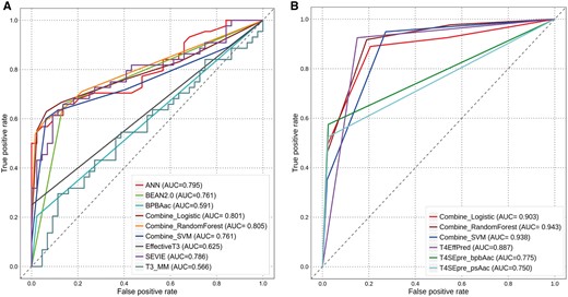
ROC-curve analysis of the predictive performance of the three ensemble-learning models as compared with all other individual predictors. (A) performance comparison between different methods for T3SE prediction using the independent test data set; (B) performance comparison between different methods for T4SE prediction using the independent test data set.
Case study
To examine the scalability and robustness of the reviewed predictors, we performed a case study using experimentally verified examples that were not included in both the training and testing data sets. The case studies for T3SEs and T4SEs were conducted separately by submitting the protein sequences to the corresponding web servers or by using stand-alone software. The detailed prediction output from each tool can be found in the Supplementary Data.
The first case study proteins were the E3 ubiquitin-protein ligase SlrP (NCBI ID: 81853756; UniProt ID: Q8ZQQ2) and the T3SS cytotoxic effector BteA (NCBI ID: 633380306). SlrP is a Salmonella T3SE that mimics host cell factors in the ubiquitination pathway, thereby resulting in host-cell death [97]. Most of the existing T3SE predictors, including the ensemble-learning models succeed to correctly predict SlrP as a T3SE. Only Effective T3 failed to predict its identity. BteA (Bordetella type 3 secretion system effector A) is a Bordetella T3SE that is a non-apoptotic cytotoxic effector for a wide range of mammalian cells [98]. The existing T3SE predictors, including BPBAac, Effective T3 and SIEVE failed to predict BteA as a T3SE, while ANN, BEAN 2.0, T3_MM and the ensemble-learning models correctly predicted BteA as a T3SE.
The second case study proteins were the E3 ubiquitin-protein ligase LubX (UniProt ID: Q5ZRQ0) and the product of the gene Lwal_1306 (UniProt ID: A0A0W1AD05), which is a T4SE secreted by the Dot/Icm T4SS of Legionella waltersii but of unknown cellular function [20]. LubX is a Legionella T4SE that interferes with the host cell ubiquitination pathway, thereby resulting in host-cell death [99]. The existing tools, including the ensemble-learning models, correctly predicted LubX as a T4SE, except for T4SEpre_joint. In the case of Lwal_1306, only T4Effpred and the ensemble-learning models successfully predicted its identity as a T4SE.
These results highlight the inconsistencies in existing prediction tools, and the importance and value of integrating the prediction outputs of individual tools into the ensemble-learning models to obtain reliable T3SE and T4SE predictions.
Conclusion
The biological significance of effector proteins has motivated the development of computational tools that facilitate accurate predictions of T3SEs, T4SEs and T6SEs. The development of such tools enables comprehensive study of host–pathogen interactions as well as characterization of the arsenal of specific effectors delivered in any given scenario of bacterial infection and virulence. In this study, we performed a comprehensive survey, benchmarking the performance of available methods and tools for the prediction of three major types of bacterial effector proteins: T3SEs, T4SEs and T6SEs. Additionally, we reviewed, discussed and assessed all methods in terms of their learning algorithms, feature extraction and selection methods, predictive performance, their user-friendliness and applicability and availability as either a web server or stand-alone software. To provide an objective evaluation of the performance, we curated independent test data sets for the three types of effector proteins. According to cross-validation tests, BEAN 2.0 achieved the overall best performance of T3SEs prediction, while T4Effpred was the best-performing tool for T4SE prediction. Our analysis also showed that T6SE prediction remains a challenging task, still to be addressed; there remains a strong case for the development of specialized models for T6SE prediction. We suggest that by integrating the output of individual predictors, ensemble-learning models using SVMs, RF and LR methods significantly outperformed all individual tools. These ensemble methods are now available to the research community and will provide reliable and robust predictive performance for both T3SEs and T4SEs. This study serves as a useful guide for researchers who are particularly interested in using existing tools and in developing new computational methods for effector prediction. We expect that our proposed methods, along with the increasing availability of experimentally verified data and the advancement of probabilistic learning techniques, will greatly improve the prediction of bacterial effector proteins. The latter will prove invaluable for further investigations of T3SS- and T4SS-mediated pathogenesis and their roles in pathogen–host interactions.
This work provides a comprehensive review and assessment of currently available bioinformatics tools for the prediction of secreted effectors of bacteria with secretion system types III, IV and VI. We focus on prediction algorithms, prediction performance, feature selection and software utilities.
We use extracted motif patterns to assess the performance of simplified predictors for secreted effector proteins of the recently identified type VI secretion system. Our assessment was based on a curated, independent test data set.
Performance benchmarks indicate that current tools achieve a relatively satisfying performance for predicting effector proteins of the type III secretion system, while that for the type IV secretion system requires improvement.
We propose and built new ensemble models based on support vector machines, random forest and logistic regression to further improve the prediction performance of effector proteins of both the type III and type IV secretion systems. This required the integration of outputs from all individual models. Five-fold cross-validation and independent tests demonstrate that the ensemble models outperform all reviewed predictors of types III and IV secretion systems. Specific test cases are presented.
Yi An is currently a master’s student in the College of Information Engineering, Northwest A&F University, China. As a current visiting student at the Biomedicine Discovery Institute and Department of Microbiology at Monash University, she is undertaking a bioinformatics project focused on computational analysis of bacterial secreted effector proteins. Her research interests include bioinformatics, data mining and web-based information systems.
Jiawei Wang received his master’s degree in School of Electronic and Computer Engineering from Peking University, China. His research interests are bioinformatics, machine learning and data mining.
Chen Li received his PhD degree in Bioinformatics in 2016 from Monash University, Australia. He is currently a postdoctoral research fellow at the Department of Microbiology and Biomedicine Discovery Institute, Monash University, Australia. His research interests focus on systems pharmacology, bioinformatics, systems biology, machine learning and data mining.
André Leier received his PhD in Computer Science (Dr. rer. nat.) from the University of Dortmund, Germany. He conducted postdoctoral research at The Memorial University of Newfoundland, Canada, The University of Queensland, Australia, and ETH Zürich, Switzerland. He is a senior research fellow and independent research scientist at the Okinawa Institute of Science and Technology, Japan. His research interests include computational and systems biology, biomedical informatics and computational medicine.
Tatiana Marquez-Lago received her PhD in Mathematics with distinction from the University of New Mexico in 2006. She conducted postdoctoral research at The University of Queensland, Australia, and ETH Zürich, Switzerland. She is an Assistant Professor and Head of the Integrative Systems Biology Unit at the Okinawa Institute of Science and Technology, Japan. Her research interests include stochastic and multi-scaled models, systems biology, synthetic biology and biomedical informatics.
Jonathan Wilksch received his PhD degree in 2012 from The University of Melbourne, Australia. He is currently a Research Fellow in the Department of Microbiology at Monash University, Australia. His research background and current interests include the mechanisms of bacterial pathogenesis, biofilm formation, gene regulation and host–pathogen interactions.
Yang Zhang received his PhD degree in Computer Science and Engineering in 2015 from Northwestern Polytechnical University, China. He is currently a professor in the College of Information Engineering, Northwest A&F University, China. His research interests are big data analysis, machine learning and data mining.
Geoffrey I. Webb received his PhD degree in 1987 from La Trobe University. He is a professor in the Faculty of Information Technology and director of the Monash Institute for Data Science at Monash University. His research interests include machine learning, data mining, computational biology and user modelling.
Jiangning Song is a senior research fellow in the Biomedicine Discovery Institute and the Department of Biochemistry and Molecular Biology, Monash University, Australia. He is also a Principal Investigator at the Tianjin Institute of Industrial Biotechnology, Chinese Academy of Sciences. He received his PhD degree in 2005 from Jiangnan University, China and conducted his postdoctoral research at The University of Queensland, Australia and Kyoto University, Japan. His research interests include bioinformatics, systems biology, machine learning, systems pharmacology and enzyme engineering.
Trevor Lithgow received his PhD degree in 1992 from La Trobe University. He is an ARC Australian Laureate Fellow in the Biomedicine Discovery Institute and the Department of Microbiology at Monash University, Australia. His research interests particularly focus on molecular biology, cellular microbiology and bioinformatics. His laboratory develops and deploys multidisciplinary approaches to identify new protein transport machines in bacteria, understand the assembly of protein transport machines and dissect the effects of antimicrobial peptides on antibiotic resistant ‘superbugs’.
Acknowledgements
T.M.L and A.L would like to thank the Isaac Newton Institute for Mathematical Sciences.
Funding
The National Health and Medical Research Council of Australia (NHMRC) (1092262) and the Australian Research Council (ARC). G.I.W. is a recipient of the Discovery Outstanding Research Award (DORA) of the Australian Research Council (ARC). T.L. is an ARC Australian Laureate Fellow.
References
Author notes
The Yi An, Jiawei Wang and Chen Li authors contributed equally to this work.
