Structural mapping: how to study the genetic architecture of a phenotypic trait through its formation mechanism

Abstract

INTRODUCTION

The final phenotype of a trait is the consequence of interactions of its internal and external structures and processes [1, 2]. It is such a phenotype that forms the features of an organism, allowing it to survive and interact with its environment. A central theme of biology is to study the intimate association of the phenotype’s structure or form and its function or activity [3]. Structure is the basic component of the phenotype that can be understood at the molecule, cell or tissue level, whereas function refers to the capacity of how different structures are used. In order to identify the function of a phenotype, therefore, we first need to understand how the shape and properties of a structure determine its functions [4, 5].

Traditional approaches for mapping quantitative trait loci (QTLs) that control a phenotype do not consider the structural basis of the phenotype, thus failing to relate the structure of the phenotype with its function. The genetic mapping of complex traits can be improved through the dissection of the phenotypes into the underlying structural components. By measuring the structure of organic and inorganic materials, electrical impedance spectroscopy (EIS) has been increasingly used to study the function and properties of biological issues [3, 6–11]. The EIS method is based on the physical principle that the signal of alternating current (AC) will change in its amplitude and phase when it passes through a tissue, arising from the polarization and relaxation of the tissue. Based on those changes, the impedance of the tissue that is composed of a real (resistance) and an imaginary part (reactance) in a complex plane can be determined. When the real and imaginary part is measured at different frequencies, an impedance spectrum is observed [9]. Because the proportion of the AC passing through the tissue depends on its frequency and the tissue properties, such as plasma membranes, cell volumes and intra and extracellular conductivities, the electrical impedance of the tissue at a series of frequencies provides information about the cell population.

It has been observed that intracellular resistance is highly correlated with physiological and pathological variables of tissues, such as frost hardiness [8, 9] and cancer risk [3, 10], through changes in cellular features and processes. With a proper equivalent electrical model, it is possible to study the tissue properties according to the changes in the parameters of the model [12]. In this article, we describe and assess a computational model—structural mapping—for mapping specific QTLs that determine the function of complex traits using EIS parameters that quantify tissue properties. In the EIS analysis, a number of robust mathematical models have been established to describe the dynamic properties of impedance through the tissue [7, 13, 14]. These models are integrated with genetic mapping derived to map dynamic QTLs [15–17], characterizing the genetic effects of QTLs on the trait by testing the mathematical parameters. Structural mapping is shown to be powerful for mapping internal structural properties of phenotypic formation and can be used to study the genetic control mechanisms of structural–functional relationships that pervade the kingdom of biology.

MODEL

EIS modeling

The biological features of a tissue can be quantified by an equivalent electrical circuit analysis [9, 13]. The impedance spectra of tissues can be viewed as an equivalent circuit with two distributed circuit elements (DCE₁ and DCE₂) in series with a resistor R (Figure 1) [9]. Below, we describe this double-DCE model, which is mostly derived from Repo et al. [9]. Both DCE-elements consist of a parallel arrangement of a resistor R₁ and R₂ and a constant phase element and respectively. According to Macdonald [13], the impedance of the constant phase elements (CPEs) is expressed as:

where ω = 2πt is the angular velocity (t is the frequency), ϕ is the imaginary unit, C₁ and C₂ are the specific capacitance for DCE₁ and DCE₂, respectively, and ψ₁ and ψ₂ are two distribution coefficients of the relaxation times for the two DCEs.

Figure 1:

Schematic determination of the distributed model parameters (double-DCE) of an impedance spectrum of a tissue (shown by open diamond). Real part of impedance on x-axis and imaginary part of impedance on y-axis (A). Frequency increases from right (80 Hz) to left (1 MHz). The two circles represent the two arcs of the spectrum. DCE1 and DCE2 are distributed circuit elements composed of constant phase elements (CPE) in parallel with resistors (B). Resistances (R, R₁ and R₂) of the equivalent model are obtained according to the intersections of the circles with x-axis. The centre of the circles is below x-axis—‘depressed center’ defined by parameters ψ₁ andψ₂. Relaxation times τ₁ and τ₂ are obtained from the apex of the circles. Z_CPE1 and Z_CPE2 are impedances of constant phase elements. Adapted from Repo et al. [9].

Open in new tabDownload slide

The impedance of the DCEs can be derived as:

where R₁ and R₂ are two resistances in the double-DEC model, by using the relationships:

Letting and which are two relaxation times of the DCEs, we have:

Thus, the total complex impedance of the double-DCE is expressed as:

(1)

where the real part is

and the imaginary part is

In sum, the double-DCE model contains three resistances (R, R₁ and R₂), two relaxation times (τ₁ and τ₂) and two distribution coefficients (ψ₁ and ψ₂) of the relaxation times. Mathematical interpretations of all these parameters are diagrammed in Figure 1.

Regression model

Consider a backcross population of n progeny in which a panel of markers are genotyped and EIS values are measured at T frequencies. Assume that a set of QTLs (forming a total of J genotypes) affect EIS curves in this population. We denote the total complex impedance of progeny i at frequency t, composed of imaginary (I) and real (R) part, as Structural mapping integrates the double-DCE (1) into a statistical model for QTL mapping, expressed as:

(2)

where y_i(t) is the complex impedance value of progeny i at frequency t; z_ij is an indicator variable with z_ij = 1 if progeny i has the jth QTL genotype and z_ij = 0 otherwise; are a set of EIS parameters for QTL genotype j; and e_i(t) is a residual error distributed as a complex normal distribution with mean 0 and variance σ². The complex vector can be divided into two T-dimensional subvectors, one for the real part and the other for the imaginary part. For simplicity, we assume that the two parts are not correlated, but each part follows a multivariate normal distribution. Therefore, the phenotype vector y_i(t) has the structure of covariance matrix, expressed as:

(3)

where and are the variances of real and imaginary parts, respectively; and Σ₁ and Σ₂ are the corresponding correlation matrices. There are many approaches which can model the covariance structure. Here, the first-order autoregressive [AR(1)] model is used, i.e.

(4)

where ρ₁ and ρ₂ (−1 < ρ₁, ρ₂ < 1) are the proportion parameters with which the correlations decay with frequency lag.

Mixture model

QTL genotypes are unknown, but can be inferred from marker genotypes (M) and phenotypes (y). To do that, structural mapping is founded on a mixture model, expressed as:

(5)

where Ω contains the unknown parameters being estimated for the impedance values of different QTL genotypes, QTL positions, and residual (co)variances; is the conditional probability of QTL genotype j, conditional on the genotypes of the two flanking markers of progeny i [18]; and is a probability density function of multivariate complex normal distribution expressed as:

(6)

where μ_j is the mean vector of y_i if it has the jth QTL genotype; and and stand for the real and imaginary parts of a complex vector, respectively.

Parameter estimation

In QTL mapping, we usually estimate QTL-effect parameters by assuming the QTL at a particular position in the marker interval. This procedure is repeated throughout the entire linkage group, allowing the likelihood profile to be drawn. The peak of the profile over the map position is the estimated location of the putative QTL. This approach is used for structural mapping by fixing both the QTL position and residual correlations, ρ₁ and ρ₂ (since the correlations have a defined interval [−1,1]). We then implement the EM algorithm to estimate the other parameters related to the genotype-specific impedance values and the variances. Denote for QTL genotype j and use the first-order Taylor expansion to approximate μ_j by:

By differentiating the log likelihood with respect to the unknown parameters and setting the derivatives to equal 0, we obtain:

(7)

where

(8)

Therefore, the maximum likelihood estimates (MLEs) of θ_j can be obtained by an iterative procedure; i.e. for the sth iteration, we have

(9)

The procedure for solving equivalent circuit EIS parameters are described as follow. Let

and

We then have the tth element of the real and imaginary part of μ_j expressed as:

and

The derivatives of the tth element of R(μ_j) and I(μ_j) with respective to parameters R_j, R_1j, τ_1j, ψ_1j, R_2j, τ_2j and ψ_2j can be obtained, which are shown in Box 1. By solving the equations, we obtain the estimates of the EIS parameters for different QTL genotypes.

Box 1 The derivatives.

The derivatives of the tth element of R(μ_j) and I(μ_j) with respective to parameters R_j, R_1j, τ_1j, ψ_1j, R_2j, τ_2j and ψ_2j are obtained as:

Similarly, we can get the MLEs of and given the other parameters, as:

(10)

In the E-step, a posterior probability of progeny i that has a QTL genotype j is calculated as Equation (9). In the M-step, the parameters are estimated by Equations (9) and (10). This procedure is repeated until the iterative value of each parameter converges. The SEs of the MLEs can be estimated by using the inverse of the Fisher information matrix.

Hypothesis tests

Structural mapping is powerful for many biologically meaningful hypothesis tests. The first hypothesis is about the existence of any QTL affecting the impedance at a specific position on genome, which is formulated as:

(11)

where the H₀ corresponds to the reduced model, in which the data are fitted by assuming that no QTLs exist, and the H₁ corresponds to the full model (2). The log-likelihood ratio (LR) of the full model over the reduced model is applied to test the above hypotheses:

(12)

where and denote the MLEs of the unknown parameters under the H₀ and H₁, respectively. If a high peak of LR profiles exceeds a critical threshold, then a QTL that controls the curve of the electrical impedance on the complex plane is asserted to exist in a marker interval. The genome-wide critical threshold is determined by performing permutation tests [19].

The merit of the model also lies in the test of a number of physiologically meaningful properties of tissues. Each of the equivalent circuit EIS parameters contained within a distributed model of the tissues [1] has a particular biological mean. For example, the relaxation times, τ₁ and τ₂, describe the peak of the high-frequency arc of the impedance spectrum, which are highly correlated with frost hardiness, and ψ₁ and ψ₂ are the distribution coefficients of the relaxation times.

At low frequencies, the current may not pass through the cell membranes but flows in the apoplastic space of tissues (for plants). Thus, the extracellular resistance (R_E) is calculated as:

(13)

But the high-frequency current may pass the cell membranes and, thus, flows in both the apoplastic and symplastic space, in which case the intracellular resistance (R_I) is calculated as:

(14)

It is interesting to test how the QTLs detected control each of these parameters by formulating the null hypothesis, and respectively, for The LR test statistics are calculated to compare against the critical values for the significance determination.

RESULTS

Worked example

We described a statistical model for structural mapping that capitalizes on the capacity of the EIS device to quantify the biological and physiochemical features of a tissue by an equivalent electrical circuit analysis [9]. To validate the ability of structural mapping to map a phenotypic trait from its structural underpinnings, we implemented the algorithm to analyze a mapping data collected from a controlled cross between two heterozygous parents in Chinese jujube (Zizyphus jujuba Mill.) [20]. A male tree Dongzao (Z. jujuba Mill, cv: Dongzao) was pollinated to a female tree Linyilizao (Z. jujuba Mill, cv: Linyilizao) to generate a full-sib family. A mapping population of 150 individuals from this family was established by genotyping 423 molecular markers to construct two parent-specific linkage maps. Thus, a pseudo-test backcross design is used for QTL mapping [21]. Part of the mapping population (86 hybrids) were measured for EIS at 31 different frequencies (300 Hz to 4 MHz) with a dual trace oscilloscope using shoots under a range of temperatures (–4 to 20°C). Electrical impedance was displayed as real (resistive component) and imaginative (capacitive reactance component) parts.

Figure 2 illustrates Cole–Cole impedance plots that describe the imaginary versus real complex plane for these hybrids. Here, the imaginary part of the complex impedance of the stems under study is plotted against the real part, each curve being a function of the frequency characterized by one hybrid. The imaginary part changes with the part par in a hyperbolic manner. The impedance spectra of each hybrid can be viewed as an equivalent circuit with two DCEs. The variation of Cole–Cole impedance plots among different hybrids increases dramatically with increasing frequency, implying a possible involvement of QTLs for electrical impedance spectra.

Figure 2:

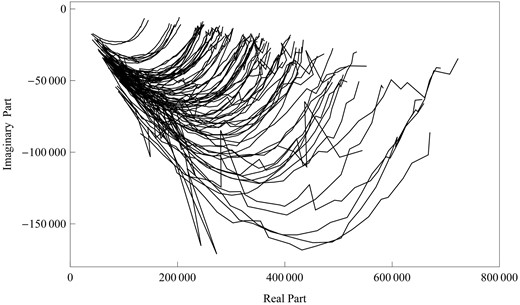
Cole–Cole plots for 86 mapping hybrids in Chinese jujube trees, composed of the imaginary part and real part.

Open in new tabDownload slide

To ensure its homoscedasticity over frequency, both the real and imaginary data are log-transformed. By scanning for the existence of QTLs in the genome, we calculated LRs at every two 2 cM through the linkage map, obtaining an LR profile against the genome position. To simplify calculations, we used a single-DCE model which takes the first two terms of model (1). Several significant QTLs were detected to affect electrical impedance spectra at the chromosome- and genome-wide level, but only one at the genome-wide level detected on the female-based linkage map is reported here for the demonstration of the new model (Figure 3). At this QTL, two different genotypes each are described by a group of EIS parameters (R, R₁, τ₁, ψ₁). As shown in Figure 4, the two QTL genotypes display different patterns of EIS curves, suggesting the impact of this QTL on structural components of shoots.

Figure 3:

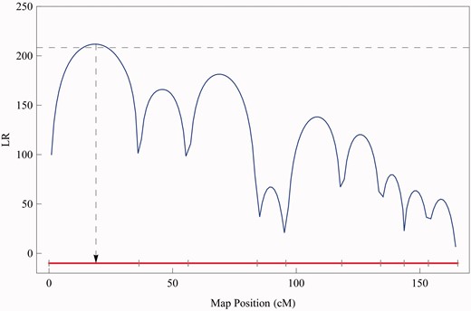
The LR profile of QTL search over a linkage group. The genome-wide critical threshold is indicated by the dash horizontal line. The LR peak corresponds to the MLE of the QTL position indicated by a of the arrowed dash vertical line. The positions of markers are indicated at ticks at x-axis.

Open in new tabDownload slide

Figure 4:

Two different curves (indicated by thick lines) for a QTL detected to affect EIS curves at the genome-wide 5% significance level. The gray curves are raw data for 86 progeny.

Open in new tabDownload slide

The EIS parameters through recalculation can be used to describe extracellular and intracellular resistances of a tissue which are related to its physiological properties such as frost hardiness. We test whether the QTL detected using our model affects extracellular and intracellular resistances of the stems of Chinese jujube. This QTL is found to display highly significant effects on both types of cellular resistance (P < 0.001). According to previous studies in tree physiology [8, 9], these two types of resistance are highly associated with frost hardiness. Our mapping population allows the distinction of two QTL-genotype groups of Chinese jujube hybrids based on the posterior probabilities of QTL genotypes given marker genotypes [18]. It is found that these two genotypes differ highly significantly in frost hardiness of jujube hybrids (P < 0.001), suggesting that results of QTL mapping with EIS can be used to diagnose the performance of trees to tolerate and resist to coldness.

Simulation

We performed a simulation study to evaluate the precision of parameter estimates, the power of structural mapping and its false positive rates using EIS data. The simulation mimics the real example analyzed above by assuming a 100-cM long linkage group with 11 equidistant markers in a backcross population. A putative QTL is assumed to be located at 46 cM from the first marker of the group. Different heritabilities (H² = 0.1, 0.4) and various sample sizes (n = 100, 200) are considered. Estimated values of the parameters from the new model are tabulated in Table 1, in a comparison with their true values used to simulate the data. It can be seen that the model provides reasonably good estimates of the model parameters, even with a modest heritability (0.1) and sample size (100). When the sample size increases to 200, the model can surely well estimate all the parameters. At a small heritability and sample size, the model displays reasonably high power for QTL detection (0.80) and low FRP (0.06). These features can improve further when a heritability and/or sample size increases.

Table 1:

Open in new tab

Means of the QTL position and MLEs of the parameters for two QTL genotypes in a pseudo-test backcross design of different sample sizes (n) under different heritabilities (H²), calculated from 200 simulation replicates. The root of mean squares errors of the estimate of each parameter is in parentheses

Parameter .	True value .	n = 100 .		n = 200 .
.	.	H2 = 0.1 .	H2 = 0.4 .	H2 = 0.1 .	H2 = 0.4 .
QTL position	46	45.95 (1.67)	45.89 (1.64)	46.02 (1.17)	45.94 (1.27)
R1	14 288.2	14 371 (1468)	14 150 (598)	14 326 (1010)	14 130 (465)
R11	132 114	131 453 (9543)	131 654 (3775)	130 699 (6574)	131 778 (2764)
τ1	3.137	3.189 (0.135)	3.148 (0.063)	3.195 (0.099)	3.146 (0.040)
ψ1	0.5256	0.526 (0.008)	0.525 (0.004)	0.526 (0.006)	0.525 (0.003)
R2	14 109	13 089 (1334)	13 963 (557)	13 092 (883)	13 875 (419)
R12	181 502	182 249 (13 212)	182 735 (5410)	182 150 (8646)	182 304 (3818)
τ2	6.862	7.225 (0.287)	6.946 (0.117)	7.240 (0.198)	6.962 (0.081)
ψ1	0.5489	0.539 (0.007)	0.547 (0.003)	0.539 (0.005)	0.546 (0.002)
ρ1	0.9994	0.999	0.999	0.999	0.999
ρ2	0.9930	0.993	0.993	0.993	0.992
	0.229	0.223 (0.033)		0.224 (0.025)
	0.263	0.279 (0.046)		0.279 (0.038)
	0.046		0.045 (0.006)		0.045 (0.005)
	0.053		0.053 (0.007)		0.05 (0.005)

Parameter .	True value .	n = 100 .		n = 200 .
.	.	H2 = 0.1 .	H2 = 0.4 .	H2 = 0.1 .	H2 = 0.4 .
QTL position	46	45.95 (1.67)	45.89 (1.64)	46.02 (1.17)	45.94 (1.27)
R1	14 288.2	14 371 (1468)	14 150 (598)	14 326 (1010)	14 130 (465)
R11	132 114	131 453 (9543)	131 654 (3775)	130 699 (6574)	131 778 (2764)
τ1	3.137	3.189 (0.135)	3.148 (0.063)	3.195 (0.099)	3.146 (0.040)
ψ1	0.5256	0.526 (0.008)	0.525 (0.004)	0.526 (0.006)	0.525 (0.003)
R2	14 109	13 089 (1334)	13 963 (557)	13 092 (883)	13 875 (419)
R12	181 502	182 249 (13 212)	182 735 (5410)	182 150 (8646)	182 304 (3818)
τ2	6.862	7.225 (0.287)	6.946 (0.117)	7.240 (0.198)	6.962 (0.081)
ψ1	0.5489	0.539 (0.007)	0.547 (0.003)	0.539 (0.005)	0.546 (0.002)
ρ1	0.9994	0.999	0.999	0.999	0.999
ρ2	0.9930	0.993	0.993	0.993	0.992
	0.229	0.223 (0.033)		0.224 (0.025)
	0.263	0.279 (0.046)		0.279 (0.038)
	0.046		0.045 (0.006)		0.045 (0.005)
	0.053		0.053 (0.007)		0.05 (0.005)

The parameters include three types: (i) the position of QTL, (ii) QTL effects specified by genotype-specific DCE parameters and (iii) AR(1) parameters.

Table 1:

Open in new tab

Means of the QTL position and MLEs of the parameters for two QTL genotypes in a pseudo-test backcross design of different sample sizes (n) under different heritabilities (H²), calculated from 200 simulation replicates. The root of mean squares errors of the estimate of each parameter is in parentheses

Parameter .	True value .	n = 100 .		n = 200 .
.	.	H2 = 0.1 .	H2 = 0.4 .	H2 = 0.1 .	H2 = 0.4 .
QTL position	46	45.95 (1.67)	45.89 (1.64)	46.02 (1.17)	45.94 (1.27)
R1	14 288.2	14 371 (1468)	14 150 (598)	14 326 (1010)	14 130 (465)
R11	132 114	131 453 (9543)	131 654 (3775)	130 699 (6574)	131 778 (2764)
τ1	3.137	3.189 (0.135)	3.148 (0.063)	3.195 (0.099)	3.146 (0.040)
ψ1	0.5256	0.526 (0.008)	0.525 (0.004)	0.526 (0.006)	0.525 (0.003)
R2	14 109	13 089 (1334)	13 963 (557)	13 092 (883)	13 875 (419)
R12	181 502	182 249 (13 212)	182 735 (5410)	182 150 (8646)	182 304 (3818)
τ2	6.862	7.225 (0.287)	6.946 (0.117)	7.240 (0.198)	6.962 (0.081)
ψ1	0.5489	0.539 (0.007)	0.547 (0.003)	0.539 (0.005)	0.546 (0.002)
ρ1	0.9994	0.999	0.999	0.999	0.999
ρ2	0.9930	0.993	0.993	0.993	0.992
	0.229	0.223 (0.033)		0.224 (0.025)
	0.263	0.279 (0.046)		0.279 (0.038)
	0.046		0.045 (0.006)		0.045 (0.005)
	0.053		0.053 (0.007)		0.05 (0.005)

Parameter .	True value .	n = 100 .		n = 200 .
.	.	H2 = 0.1 .	H2 = 0.4 .	H2 = 0.1 .	H2 = 0.4 .
QTL position	46	45.95 (1.67)	45.89 (1.64)	46.02 (1.17)	45.94 (1.27)
R1	14 288.2	14 371 (1468)	14 150 (598)	14 326 (1010)	14 130 (465)
R11	132 114	131 453 (9543)	131 654 (3775)	130 699 (6574)	131 778 (2764)
τ1	3.137	3.189 (0.135)	3.148 (0.063)	3.195 (0.099)	3.146 (0.040)
ψ1	0.5256	0.526 (0.008)	0.525 (0.004)	0.526 (0.006)	0.525 (0.003)
R2	14 109	13 089 (1334)	13 963 (557)	13 092 (883)	13 875 (419)
R12	181 502	182 249 (13 212)	182 735 (5410)	182 150 (8646)	182 304 (3818)
τ2	6.862	7.225 (0.287)	6.946 (0.117)	7.240 (0.198)	6.962 (0.081)
ψ1	0.5489	0.539 (0.007)	0.547 (0.003)	0.539 (0.005)	0.546 (0.002)
ρ1	0.9994	0.999	0.999	0.999	0.999
ρ2	0.9930	0.993	0.993	0.993	0.992
	0.229	0.223 (0.033)		0.224 (0.025)
	0.263	0.279 (0.046)		0.279 (0.038)
	0.046		0.045 (0.006)		0.045 (0.005)
	0.053		0.053 (0.007)		0.05 (0.005)

The parameters include three types: (i) the position of QTL, (ii) QTL effects specified by genotype-specific DCE parameters and (iii) AR(1) parameters.

DISCUSSION

The electrical properties of tissues in a range of frequencies are associated with the cellular components and the dimensions, internal structure and arrangements of the constituent cells [3]. Therefore, tissues with different cellular structures will produce impedance spectra characteristic of these issues. By analyzing electrical properties of biological tissues, we can better understand their structure and function. More recently, EIS has been increasingly used to study the electrical impedance of various tissues over a frequency range and determine their frequency-dependent electric and dielectric behavior [3, 6–11], providing scientific guidance for prognosis, diagnosis and prevention. The use of impedance spectroscopy electrical characterization is a novel approach to comprehend the genetic architecture of phenotypic traits underlying pathology and complex diseases.

We described a computational model for structural mapping by taking into account the structural components of phenotypic traits using EIS information. Structural mapping incorporates the electrical properties of phenotypic formation into a genetic mapping framework by which the genetic control of complex traits can be studied from a mechanistic perspective. Structural mapping was used to analyze a mapping data collected for an experimental cross of outcrossing tree species, Chinese jujube. Significant QTLs were detected to affect the complex impedance of shoots, some of which were also detected by mapping frost hardiness [20]. Because there is a strong correlation between intracellular resistance and frost hardiness [8, 9], the detection of pleiotropic QTLs for these two traits can well confirm the validation of our model. The simulation study by mimicking the real example provides a justification of statistical properties of the model.

The EIS-based structural mapping model can be expanded to study the comprehensive genetic architecture of complex traits using genome-wide association study. More specifically, structural mapping (2) should involve the impacts of genetic interactions [22], genetic imprinting [23], epigenetic marks [24] and copy number variation [25] on phenotypic variation. Furthermore, structural mapping can also be used to study phenotypic response to different environmental factors, such as temperature [8, 9] through studying the genetic architecture of phenotypic plasticity to a range of environments. By constructing a logistic sigmoid function, we can determine the biological properties of a tissue, such as frost hardiness, based on extracellular resistance over a series of temperatures. This model is expressed as:

where y and x are the specific extracellular resistance and the exposure temperature, respectively, A and D define asymptotes of the function, and B is the slope at the inflection point C. The frost hardiness is estimated as the inflection point of the above logistic function [9]. Thus, by incorporating the above logistic function, structural mapping can directly detect specific QTLs associated with frost hardiness through structural dissection.

FUNDING

This work is partially supported by Special Fund for Forestry Scientific Research in the Public Interest (No. 201004017); NSF/IOS-0923975; Changjiang Scholars Award and ‘Thousand-Person Plan’ Award.

References