


Abstract
Compared with other plant lineages, bryophytes have very small genomes with little variation across species, and high levels of endopolyploid nuclei. This study is the first analysis of moss genome evolution over a broad taxonomic sampling using phylogenetic comparative methods. We aim to determine whether genome size evolution is unidirectional as well as examine whether genome size and endopolyploidy are correlated in mosses.
Genome size and endoreduplication index (EI) estimates were newly generated using flow cytometry from moss samples collected in Canada. Phylogenetic relationships between moss species were reconstructed using GenBank sequence data and maximum likelihood methods. Additional 1C-values were compiled from the literature and genome size and EI were mapped onto the phylogeny to reconstruct ancestral character states, test for phylogenetic signal and perform phylogenetic independent contrasts.
Genome size and EI were obtained for over 50 moss taxa. New genome size estimates are reported for 33 moss species and new EIs are reported for 20 species. In combination with data from the literature, genome sizes were mapped onto a phylogeny for 173 moss species with this analysis, indicating that genome size evolution in mosses does not appear to be unidirectional. Significant phylogenetic signal was detected for genome size when evaluated across the phylogeny, whereas phylogenetic signal was not detected for EI. Genome size and EI were not found to be significantly correlated when using phylogenetically corrected values.
Significant phylogenetic signal indicates closely related mosses have more similar genome sizes and EI values. This study supports that DNA content in mosses is defined by small genomes that are highly endopolyploid, suggesting strong selective pressure to maintain these features. Further research is needed to understand the functional significance of DNA content evolution in mosses.
INTRODUCTION
Phylogenetic comparative methods provide a powerful tool to enhance our understanding of genome size (1C-value, the amount of DNA in a non-replicated chromosome complement; Greilhuber et al., 2005) evolution across land plants (Leitch et al., 2005; Soltis et al., 2018). Phylogenetic reconstructions indicate that the ancestral genome size of land plants was likely very small (Soltis et al., 2018), with larger genome sizes subsequently evolving in many plant lineages e.g. lycophytes (Bainard et al., 2011a); ferns (Clark et al., 2016), gymnosperms (Burleigh et al., 2012) and angiosperms (Leitch et al., 1998)]. In contrast, the three bryophyte lineages (hornworts, liverworts and mosses) predominantly retain the very small ancestral genome sizes with little variation across species (Temsch et al., 1998; Voglmayr, 2000; Bainard and Villarreal, 2013; Bainard et al., 2013). While considerable genome size data have been amassed for all three bryophyte lineages, a comprehensive analysis of genome size evolution using phylogenetic comparative methods is lacking for mosses.
Mosses (Bryophyta) are the most speciose bryophyte lineage, comprising ~13 000 species worldwide (Magill, 2010), compared with liverworts (Marchantiophyta) with 7271 species and hornworts (Anthocerotophyta) with 215 species (Söderström et al., 2016). These lineages share a dominant haploid generation in the course of alternation of generations, with an unbranched sporophyte that remains physically attached to and nutritionally dependent on the maternal gametophyte throughout its lifespan. Recent analyses of molecular data have confirmed the longstanding hypothesis of a sister relationship between liverworts and mosses (setaphyte hypothesis), which was first proposed based on morphological studies of spermatogenesis (Renzaglia and Garbary, 2001; Renzaglia et al., 2018), and have also supported the monophyly of the three bryophyte lineages (Morris et al., 2018; Puttick et al., 2018; de Sousa et al., 2019). Analysing the 1C-values present in mosses will broaden our understanding of genome size evolution in bryophytes and across land plants.
Overall, <1.5 % of known moss species have published genome size estimates (Plant DNA C-values Database; http://data.kew.org/cvalues/) and the need to better understand genome diversity in this lineage has often been noted (e.g. Leitch and Leitch, 2013). Voglmayr (2000) can be credited with the largest single survey of moss species to date, which contained 138 taxa. Genome sizes for Sphagnum (peat mosses) have been reported by Temsch et al. (1998), Greilhuber et al. (2003) and Karlin et al. (2014). A handful of other moss species have published genome size estimates (Reski et al., 1994; Renzaglia et al., 1995; Lamparter et al., 1998; Zouhair and Lecocq, 1998; Schween et al., 2003; Melosik et al., 2005; Bainard et al., 2010).
Bryophytes have both very small and more highly constrained genome sizes in comparison with other land plants (Soltis et al., 2018). The greatest variation in genome sizes is found in the angiosperms, which range in 1C-value from 61 Mbp (0.06 pg) in Genlisea tuberosa (Fleischmann et al., 2014) to 148 852 Mbp (152.23 pg) in Paris japonica (Pellicer et al., 2010). The monilophytes (ferns) show a similar wide range in genome sizes, from 750 Mbp (0.8 pg) in Azolla microphylla (Obermayer et al., 2002) to 147 297 Mbp (150.61 pg) in Tmesipteris obliqua (Hidalgo et al., 2017), while the lycophytes (fern allies) range from 81 Mbp (0.08 pg) in Selaginella selaginoides (Baniaga et al., 2016) to 11 704 Mbp (11.97 pg) in Isoetes lacustris (Hanson and Leitch, 2002). Gymnosperms tend to have larger genomes on average, ranging from 2201 Mbp (2.25 pg) in Gnetum ula (Ohri and Khoshoo, 1986) to 35 208 Mbp (36 pg) in Pinus ayacahuite (Grotkopp et al., 2004). Across bryophytes, 1C-values for hornworts range from only 160 Mbp (0.16 pg) in Leiosporoceros dussii to 719 Mbp (0.73 pg) in Nothoceros endiviifolius (Bainard and Villarreal, 2013), while liverworts have a wider variation of sizes, from 206 Mbp (0.21 pg) in Lejeunea cavifolia (Temsch et al., 2010) to 20 006 Mbp (20.46 pg) in Phyllothallia fuegiana (Bainard et al., 2013). The variation in moss genome sizes falls between the other two bryophyte lineages and spans from 170 Mbp (0.17 pg) in Holomitrium arboreum to 2004 Mbp (2.05 pg) in Mnium marginatum (Voglmayr, 2000).
DNA content varies within an individual plant when nuclei are found at varying ploidy levels in the same individual, termed endopolyploidy (Nagl, 1978). Endopolyploidy is the result of endoreduplication, which occurs when DNA replication is not followed by mitotic division, and is largely due to modification of cyclin-dependent kinase activity (De Veylder et al., 2011). The prevalence of endopolyploidy varies widely across plant lineages. It is common in angiosperms and mosses, appears to be rare in both gymnosperms and ferns, and is entirely lacking in liverworts (Barlow, 1978; Barow and Jovtchev, 2007; Bainard and Newmaster, 2010). High levels of endopolyploidy are often associated with small genome sizes in plants (Nagl, 1978; De Rocher et al., 1990; Barow and Meister, 2003; Bainard et al., 2012). The implications of this relationship may have far-reaching consequences, as the amount of DNA (the ‘nucleotype’) directly impacts nuclear and cell volume, which in turn affects other morphological and ecological features (Bennett, 1971, 1972; Cavalier-Smith, 1978). Barow and Meister (2003) speculated that endopolyploidy in angiosperms may allow species with small genomes to combine the advantages of a small genome (such as shorter cell cycles and shorter generation times) with those of a large genome (such as the ability for cell growth and expansion in low temperatures). All mosses surveyed to date, except for members of the genus Sphagnum, demonstrate high levels of endopolyploidy (Bainard and Newmaster, 2010). Understanding whether there is a relationship between genome size and endopolyploidy in mosses will help us determine if this pattern is limited to broad differences within the angiosperm lineage, or if it occurs in other taxonomic groups as well.
We tested the following hypotheses using the most comprehensive dataset of 1C-values and endopolyploidy data assembled to date from a broad phylogenetic sample of moss species. (1) We tested the genetic obesity hypothesis (Bennetzen and Kellogg, 1997), which postulates that genome size evolution is unidirectional, resulting in species with larger genomes occupying derived positions within the phylogeny. (2) We examined whether there is phylogenetic signal for genome size and/or endopolyploidy, which is the tendency of closely related species to resemble each other more than a random set of species from the same tree (Harvey and Pagel, 1991). (3) We tested the hypothesis that high levels of endopolyploidy are correlated with small genome sizes (Nagl, 1978; De Rocher et al., 1990; Barow and Meister, 2003), using phylogenetic comparative methods that account for the non-independence of data collected across species (Felsenstein, 1985).
MATERIALS AND METHODS
Plant material
Moss specimens were collected from three main localities in Canada in the summer of 2009: various sites in Ontario, the Gulf Islands in British Columbia, and Churchill, Manitoba. Species were identified by the authors using floras appropriate for each region (Lawton, 1971; Crum and Anderson, 1981). Voucher specimens of all collected materials are deposited in the Biodiversity Institute of Ontario Herbarium (OAC/BIO, University of Guelph; Supplementary Data Table S1). Sampling for this study was limited to field-collected populations. Laboratory-cultured populations for additional Funariaceae species were originally included in the sampling; however, Schween et al. (2003) found that cultured mosses have a majority of nuclei in the G2/M phase in the juvenile chloronema cells, and very few (sometimes lacking) nuclei in G1/S phase in caulonema cells. This made it very difficult to determine the 1C nuclei in a flow cytometry histogram and thus these laboratory cultures of Funariaceae were excluded from this study. Before analysis, the moss gametophyte tissue was air-dried, which does not significantly affect DNA content estimates (Bainard et al., 2010; Bainard et al., 2011b). Leaf and stem tissue that was green and healthy was selected for analysis. After mosses were determined suitable for analysis by flow cytometry, there was a total of 60 samples: 39 from Ontario, 14 from British Columbia and seven from Manitoba (Table 1).
DNA content estimates for moss species collected at various locations in Canada (BC, British Columbia; MB, Manitoba; ON, Ontario). Taxa are classified according to the Taxonomic Name Resolution Service (http://tnrs.iplantcollaborative.org) and are arranged alphabetically by family. Genome size is reported as average 1C-value ± standard error of the mean in picograms (pg) as well as average Mbp (1 pg = 0.978 × 10⁹ bp; Doležel et al., 2003). Degree of endopolyploidy is reported as the endoreduplication index (EI) ± s.e.m.
| Taxon | Collection locality | 1C-value ± s.e.m. (pg) | 1C-value (Mbp) | Standard | EI ± s.e.m. |
|---|---|---|---|---|---|
| Amblystegiaceae | |||||
| Campylium chrysophyllum (Brid.) Lange | ON | 1.00 ± 0.022 | 982 | Solanum lycopersicum | 0.64 ± 0.057 |
| Sanionia uncinata (Hedw.) Loeske | MB | 0.37 ± 0.007 | 358 | Raphanus sativus | 1.53 ± 0.023 |
| Aulacomniaceae | |||||
| Aulacomnium androgynum (Hedw.) Schwägr. | ON | 0.34 ± 0.007 | 336 | Raphanus sativus | 0.64 ± 0.076* |
| Brachytheciaceae | |||||
| Brachythecium acuminatum (Hedw.) Austin | ON | 1.02 ± 0.022 | 999 | Glycine max | 0.54 ± 0.045* |
| Brachythecium salebrosum (Hoffm. ex F.Weber and D.Mohr) Schimp. | BC | 0.55 ± 0.004 | 534 | Glycine max | 1.01 ± 0.037 |
| Brachythecium salebrosum (Hoffm. ex F.Weber and D.Mohr) Schimp. | ON | 0.97 ± 0.057 | 952 | Glycine max | 0.14 ± 0.018* |
| Brachythecium velutinum (Hedw.) Schimp. | ON | 0.46 ± 0.004§ | 449 | Raphanus sativus | 0.51 ± 0.071* |
| Cirriphyllum piliferum (Hedw.) Grout | MB | 1.04 ± 0.009 | 1021 | Glycine max | 0.63 ± 0.056 |
| Eurhynchium pulchellum (Hedw.) Jenn. | ON | 0.52 ± 0.024 | 507 | Raphanus sativus | 0.27 ± 0.044* |
| Homalothecium aeneum (Mitt.) E. Lawton | BC | 0.26 ± 0.006 | 257 | Glycine max | 1.63 ± 0.114 |
| Pohlia wahlenbergii (F. Weber and D. Mohr) A.L. Andrews | ON | 0.49 ± 0.006 | 481 | Raphanus sativus | 1.13 ± 0.125* |
| Bruchiaceae | |||||
| Trematodon ambiguus (Hedw.) Hornsch. | ON | 0.39 ± 0.003 | 384 | Raphanus sativus | 0.51 ± 0.055* |
| Climaciaceae | |||||
| Climacium dendroides (Hedw.) F. Weber and D.Mohr | ON | 1.00 ± 0.041 | 983 | Glycine max | 1.48 ± 0.029* |
| Dicranaceae | |||||
| Dichodontium pellucidum (Hedw.) Schimp. | MB | 0.34 ± 0.005 | 329 | Raphanus sativus | 0.42 ± 0.017 |
| Dicranoweisia cirrata (Hedw.) Lindb. | BC | 0.25 ± 0.001 | 243 | Raphanus sativus | 0.57 ± 0.016 |
| Dicranum condensatum Hedw. | ON | 0.81 ± 0.026 | 795 | Raphanus sativus | 0.87 ± 0.072* |
| Dicranum flagellare Hedw. | ON | 0.57 ± 0.018 | 557 | Glycine max | 0.50 ± 0.015* |
| Dicranum fuscescens Turner | ON | 0.65 ± 0.017 | 639 | Glycine max | 0.57 ± 0.087* |
| Dicranum fuscescens Turner | BC | 0.74 ± 0.014 | 728 | Raphanus sativus | 0.44 ± 0.010 |
| Dicranum groenlandicum Brid. | MB | 0.60 ± 0.013 | 585 | Raphanus sativus | N/A |
| Dicranum montanum Hedw. | ON | 0.52 ± 0.010 | 507 | Raphanus sativus | 0.52 ± 0.029* |
| Dicranum polysetum Sw. | ON | 0.78 ± 0.027 | 758 | Raphanus sativus | 1.11 ± 0.030* |
| Dicranum scoparium Hedw. | ON | 0.38 ± 0.010 | 375 | Solanum lycopersicum | 0.98 ± 0.048* |
| Dicranum scoparium Hedw. | BC | 0.72 ± 0.013 | 709 | Raphanus sativus | 1.22 ± 0.014 |
| Dicranum spurium Hedw. | MB | 0.35 ± 0.004 | 338 | Raphanus sativus | 0.59 ± 0.029 |
| Ditrichaceae | |||||
| Ceratodon purpureus (Hedw.) Brid. | ON | 0.47 ± 0.004 | 456 | Raphanus sativus | 0.51 ± 0.060* |
| Ditrichum lineare (Sw.) Lindb. | MB | 0.35 ± 0.003 | 343 | Raphanus sativus | 0.32 ± 0.026 |
| Fissidentaceae | |||||
| Fissidens taxifolius Hedw. | ON | 0.32 ± 0.001§ | 313 | Raphanus sativus | 0.40 ± 0.039* |
| Hedwigiaceae | |||||
| Hedwigia ciliata (Hedw.) P.Beauv. | ON | 0.30 ± 0.003§ | 291 | Raphanus sativus | 0.34 ± 0.030* |
| Hylocomiaceae | |||||
| Hylocomium splendens (Hedw.) Schimp. | ON | 0.48 ± 0.003 | 471 | Raphanus sativus | 0.53 ± 0.165* |
| Pleurozium schreberi (Willd. Ex Brid.) Mitt. | ON | 0.83 ± 0.039 | 809 | Raphanus sativus | 0.35 ± 0.079* |
| Pleurozium schreberi (Willd. Ex Brid.) Mitt. | MB | 0.43 ± 0.008 | 418 | Raphanus sativus | 0.74 ± 0.028 |
| Rhytidiadelphus triquetrus (Hedw.) Warnst. | ON | 0.57 ± 0.020 | 555 | Glycine max | 0.52 ± 0.036* |
| Hypnaceae | |||||
| Callicladium haldanianum (Grev.) H.A. Crum | ON | 0.83 ± 0.023 | 816 | Raphanus sativus | 0.69 ± 0.187* |
| Calliergonella lindbergii (Mitt.) Hedenäs | ON | 0.40 ± 0.010 | 389 | Raphanus sativus | 0.78 ± 0.236* |
| Hypnum curvifolium Hedw. | ON | 0.59 ± 0.004 | 580 | Glycine max | 1.30 ± 0.107* |
| Hypnum pallescens (Hedw.) P.Beauv. | ON | 0.38 ± 0.011 | 376 | Raphanus sativus | 0.96 ± 0.078* |
| Hypnum recurvatum (Lindb. and Arnell) Kindb. | ON | 0.37 ± 0.007 | 365 | Raphanus sativus | 0.34 ± 0.104* |
| Ptilium crista-castrensis (Hedw.) De Not. | ON | 0.40 ± 0.010 | 388 | Raphanus sativus | 0.27 ± 0.016* |
| Pylaisia polyantha (Hedw.) Schimp. | ON | 0.41 ± 0.008 | 399 | Raphanus sativus | 0.37 ± 0.054* |
| Lembophyllaceae | |||||
| Isothecium cristatum (Hampe) H.Rob. | BC | 0.44 ± 0.006 | 427 | Raphanus sativus | 0.36 ± 0.021 |
| Isothecium myosuroides Brid. | BC | 0.53 ± 0.011 | 518 | Raphanus sativus | N/A |
| Leskeaceae | |||||
| Claopodium crispifolium (Hook.) Renauld and Cardot | BC | 0.40 ± 0.000 | 393 | Raphanus sativus | 0.81 ± 0.080 |
| Haplocladium microphyllum (Hedw.) Broth. | ON | 0.44 ± 0.011 | 432 | Raphanus sativus | 0.41 ± 0.086* |
| Leucodontaceae | |||||
| Antitrichia curtipendula (Timm ex Hedw.) Brid. | BC | 0.52 ± 0.002 | 507 | Solanum lycopersicum | 0.73 ± 0.017 |
| Dendroalsia abietina (Hook.) E. Britton ex Broth. | BC | 0.37 ± 0.004 | 363 | Raphanus sativus | 0.67 ± 0.139 |
| Mniaceae | |||||
| Leucolepis acanthoneura (Schwägr.) Lindb. | BC | 1.18 ± 0.010 | 1155 | Solanum lycopersicum | 0.93 ± 0.062 |
| Plagiomnium drummondii (Bruch and Schimp.) T.J. Kop. | ON | 0.63 ± 0.004 | 612 | Glycine max | 1.37 ± 0.054* |
| Plagiomnium medium (Bruch and Schimp.) T.J. Kop. | ON | 0.97 ± 0.012 | 949 | Glycine max | 1.21 ± 0.152* |
| Neckeraceae | |||||
| Metaneckera menziesii (Drumm.) Steere | BC | 0.44 ± 0.004 | 427 | Raphanus sativus | 1.13 ± 0.129 |
| Neckera douglasii Hook. | BC | 0.51 ± 0.005 | 498 | Raphanus sativus | 0.73 ± 0.074 |
| Orthotrichaceae | |||||
| Orthotrichum speciosum Nees | ON | 0.35 ± 0.009 | 343 | Raphanus sativus | 0.30 ± 0.071* |
| Plagiotheciaceae | |||||
| Plagiothecium denticulatum (Hedw.) Schimp. | ON | 0.55 ± 0.014 | 540 | Raphanus sativus | 1.05 ± 0.160* |
| Plagiothecium laetum Schimp. | ON | 0.55 ± 0.000 | 536 | Glycine max | 1.71 ± 0.062* |
| Polytrichaceae | |||||
| Polytrichastrum formosum (Hedw.) G.L. Sm. | BC | 0.67 ± 0.008 | 655 | Raphanus sativus | 0.51 ± 0.065 |
| Polytrichum commune Hedw. | ON | 1.08 ± 0.001 | 1056 | Zea mays | 0.33 ± 0.055* |
| Polytrichum juniperinum Hedw. | ON | 0.46 ± 0.019 | 455 | Raphanus sativus | 0.60 ± 0.060* |
| Sphagnaceae | |||||
| Sphagnum recurvum P. Beauv. | ON | 0.56 ± 0.012 | 549 | Raphanus sativus | 0.00 ± 0.000* |
| Thuidiaceae | |||||
| Cyrto-hypnum minutulum (Hedw.) W.Raphanus Buck & H.A. Crum | ON | 0.44 ± 0.002§ | 435 | Raphanus sativus | 0.41 ± 0.025* |
| Thuidium delicatulum (Hedw.) Schimp. | ON | 0.43 ± 0.000 | 418 | Raphanus sativus | 0.91 ± 0.119* |
§Value published in Bainard et al. (2010).
*Value published in Bainard and Newmaster (2010).
Flow cytometric analyses
To estimate genome size, methods followed Galbraith et al. (1983) as modified by Bainard et al. (2010). Seeds for standards with known DNA content were acquired from the Laboratory of Molecular Cytogenetics and Cytometry, Olomouc, Czech Republic, and the standards were grown in the University of Guelph Phytotron. The standards used in this study included: Raphanus sativus L. ‘Saxa’, 2C value = 1.11 pg (Doležel et al., 1998), Solanum lycopersicum L. ‘Stupicke polni tyckove rane’, 2C value = 1.96 pg (Doležel et al., 1992), Glycine max Merr. ‘Polanka’, 2C value = 2.50 pg (Doležel et al., 1994) and Zea mays L. ‘CE-777’, 2C value = 5.43 pg (Lysák and Doležel, 1998). Approximately 10 mg of air-dried moss gametophyte tissue (1C) was co-chopped with fresh leaf tissue (2C) from an appropriate plant standard (the fluorescence intensity of the standard G1 nuclei was within a 4-fold range of the sample G1 nuclei). Tissues were chopped in 1.2 mL of cold LB01 lysis buffer (Doležel et al., 1989), in the presence of 150 μg mL−1 propidium iodide (PI, Sigma) and 50 μg mL−1 RNase A (Sigma). The higher than average concentration of 150 μg mL−1 PI was used according to Bainard et al. (2010), where this concentration was found to be saturating (i.e. at lower concentrations the genome size was underestimated). The resulting homogenate of leaf tissues and staining solution was filtered through a 30-μm mesh (CellTrics, Sysmex) and incubated on ice for 20–40 min. For each sample, over 1000 nuclei were obtained, but in a few cases where tissue amounts were minimal fewer than 1000 nuclei were obtained per flow accession. Three independent replicates of the same moss specimen were analysed on separate days and the estimates were averaged. Where the same moss taxon was collected from distinct localities, separate estimates were obtained. To estimate genome size, the 1C nuclei of the moss (in G1 phase of the cell cycle) were compared with the 2C nuclei (G1) of the standard. Genome size was calculated by determining the ratio between the mean fluorescence intensity of the moss 1C peak and the standard 2C peak, and multiplying by the known DNA content of the standard.
To determine the degree of endopolyploidy for each moss sample, preparation methods followed those given above for genome size. (Although it is recognized that endopolyploidy can vary between different plant organs and tissues, because of the small size of mosses it is very difficult to acquire enough tissue from only leaf material, so samples included a mix of stem and leaf tissue.) If the moss nuclei could be easily counted in each endopolyploid peak from samples that were co-chopped with a standard, those replicates were used; however, in most cases an additional three replicates were prepared of the moss tissue alone, and run on separate days. On average, over 4000 nuclei were analysed over all peaks, and the number of nuclei in each ploidy level was determined. There is a small risk of misinterpreting the 2C peak as the 1C peak if there are very few nuclei in the 1C peak [as occurred in cultured samples of Physcomitrella patens (Reski et al., 1994; Schween et al., 2003)], therefore high nuclei counts were desired and all flow histograms were carefully examined. The endoreduplication index (EI), or cycle value, reports the average number of endoreduplication cycles undergone by the nuclei measured, and is calculated as:
where n is the number of nuclei in each ploidy level (Barow and Jovtchev, 2007). As moss gametophyte (1C) tissue was analysed, one endoreduplication cycle results in nuclei at the 2C level. EI values <0.1 were not considered endopolyploid (Barow and Meister, 2003; Jovtchev et al., 2006). This threshold can account for the small number of nuclei at higher ploidies that are not actually endopolyploid, but rather are due to nuclei in the G2 phase of the cell cycle or to doublet formation (nuclei stuck together).
Flow cytometric analyses were carried out on a Partec CyFlow SL (Partec, Münster, Germany) equipped with a blue solid-state laser tuned at 20 mW and operating at 488 nm. The flow cytometer was calibrated using 3-µm calibration beads (Partec, Münster, Germany) before each use. For each sample, the following parameters were observed: fluorescence intensity at 590 ± 25 nm (‘FL2’, measured on a linear scale to calculate genome size), fluorescence intensity at 630 nm (‘FL3’, measured on a log scale to calculate degree of endopolyploidy), as well as forward scatter and side scatter. In order to calculate EI and genome size from the same sample, both fluorescence parameters were measured as genome size must be measured on a linear scale, while EI could only be observed on a log scale. As PI has an emission wavelength of 617 nm (Doležel et al., 2007), both FL2 and FL3 parameters accurately report the relative fluorescence. Histograms were analysed using FloMax Software (version 2.52; Partec). The fluorescence parameters were observed alone and in combined scattergrams including: fluorescence versus side scatter and fluorescence versus forward scatter. Polygon gates were drawn on these scattergrams to separate the nuclei of interest from debris particles.
Phylogenetic analyses
Species names were standardized and the families identified for all taxa with genome size estimates analysed in this study, including both newly generated data (Table 1) and previously published values (Supplementary Data Table S2) using the online taxonomic name resolution service (Boyle et al., 2013; The Taxonomic Name Resolution Service, accessed 22 Jan 2018). Sequence data were downloaded from the NCBI database (NCBI Resource Coordinators, 2016) using SUMAC 2.22 (Freyman, 2015), which enables a bulk download of data from all species in a family. The minimum number of required sequences per cluster was set to 500 and all other settings were as default. Using these criteria, six clusters corresponding to the gene regions nad5, rbcL, trnS-rps4-trnT-trnL-trnF, trnL-trnF, 18S-ITS1-5.8S-ITS2-26S and ITS2-26S were identified. Due to the large amount of overlap between the trnS-trnF and trnL-trnF clusters, only the latter cluster was retained, with the former removed from subsequent analyses. The 18S-ITS1-5.8S-ITS2-26S and ITS2-26S clusters were combined with sequences added to the 18S-ITS1-5.8S-ITS2-26S cluster for any species missing data for this gene region from the ITS2-26S cluster. All sequences with tenuous species identifications indicated by ‘cf.’ were removed from subsequent analyses.
Sequences were clustered using the UCLUST algorithm (Edgar, 2010) in SUMAC and each of the four gene regions (nad5; rbcL; trnL-trnF; 18S-ITS1-5.8S-ITS2-26S) were independently aligned using ClustalW 1.82 (Larkin et al., 2007), then trimmed and concatenated in Geneious 9.1.8 (Kearse et al., 2012). Data partitions and models were chosen using the corrected Akaike information criterion (AICc) and the search scheme greedy in PartitionFinder2 2.1.1 (Guindon et al., 2010; Lanfear et al., 2017). Analyses were performed using RAxML 8.2.10 (Stamatakis, 2014). Alignments, model selection and analyses were carried out via the CIPRES Science Gateway (Miller et al., 2010). The resulting maximum likelihood tree was rescaled in units of time using treePL (Smith and O’Meara, 2012), which implements the penalized likelihood dating method for large phylogenies (Sanderson, 2002). The rate-smoothing parameter was determined using the randomcv option, testing five values between 0.1 and 1000 separated by one order of magnitude using cross-validation and the χ2 test Additionally, the thorough option was used to iterate until convergence, and branch lengths were scaled with the root age set to 1. Trees were rooted with the genus Sphagnum as the outgroup. Alignments and tree files were uploaded to TreeBASE (submission ID 25488).
All analyses were carried out using R version 3.4.2 (R Core Team, 2017). When multiple genome size estimates were available for a given species from the new data or published data, the smallest (most conservative) estimate was used. Genome size and EI were independently mapped onto the pruned phylogenies using the ContMap function with default settings from the phytools package (Revell, 2012). Both datasets showed skewed distributions and thus were log10-transformed prior to analysis. Pagel’s λ (Pagel, 1999) was used to test for phylogenetic signal, since this analysis was the least affected by variation in species number in comparison with other indices (Münkemüller et al., 2012). Pagel’s λ was used to test for phylogenetic signal assuming Brownian motion by optimizing the value of λ using maximum likelihood with no constraints and comparing that with the likelihood of a model where λ was constrained to zero (no phylogenetic signal) using the phylosig function from the phytools package. In addition, a phylogenetically correct linear model (Felsenstein, 1985) was used to test for a relationship between genome size and degree of endopolyploidy in mosses. This analysis only used species with a 1C-value estimate and EI determined from the same tissue sample (reported in this study or Bainard and Newmaster, 2010). Phylogenetically independent contrasts were calculated for the 1C-value estimates and EI values independently using the pic function from the ape package (Paradis et al., 2004) and then a regression through the origin using the lm function was performed on these adjusted values.
RESULTS
DNA content in mosses
Genome size estimates were acquired for 60 moss samples, representing 56 species from 20 families (Table 1). Estimates for 33 species have not previously been reported in the literature, including representatives from two additional families, Bruchiaceae and Orthotrichaceae. Across the 60 estimates of genome size, 1C-values ranged from 0.25 pg (Dicranoweisia cirrata) to 1.18 pg (Leucolepis acanthoneura) (Table 1). Quality of the flow cytometry histograms was suitable, as the coefficients of variation ranged from 2.51 to 7.94 % (mean = 4.81 %) in the moss peak and from 2.27 to 7.77 % (mean = 3.45 %) in the standard peak. While lower coefficients of variation are often recommended (e.g. less than 3 % or 5 %) it is recognized that this can be difficult when dealing with very small nuclei that approach the resolution capacity of the flow cytometer (Voglmayr, 2007).
Four moss taxa were collected from two different locations in this study, and in all cases the genome sizes were different (Table 1). All samples listed in Table 1 were personally identified by the authors to decrease the likelihood of misidentification. In three of the species (Brachythecium salebrosum, Dicranum scoparium and Pleurozium schreberi) the samples differ by almost an exact doubling, which could be attributed to variation in ploidy. In addition, the two Dicranum fuscescens samples differ by ~13 % and this variation within a single morphologically identifiable species could be attributed to convergent evolution that is obscuring a cryptic species.
Additionally, 20 moss species estimated in this study (represented by 23 accessions) also have a 1C-value estimated by Voglmayr (2000) (Table 2). As Voglmayr (2000) estimated genome size using both Feulgen staining and PI flow cytometry, we only compared values that had been obtained using PI. When comparing variation in estimates between different populations of the same species in his study, Voglmayr (2000) suggested that a ratio lower than 1.15 (maximum/minimum) was indicative of low, if any, variation in C value. Differences between estimates up to 10 % have also been considered within the margin of error in previous genome size studies (Bennett and Smith, 1976; Bennett and Leitch, 2005). When comparing our estimates with those published in Voglmayr (2000), ten accessions have a ratiomax/min lower than 1.15 (Table 2), suggesting the estimates are equivalent. Five accessions had disparate genome size estimates that were close to double or triple those of each other, which might suggest polyploidization (Table 2). In the remaining comparisons, estimates from the present study were all higher than in Voglmayr (2000).
Comparison of estimates from the current study and Voglmayr (2000). Ratiomax/min measures the ratio of the higher value divided by the lower value. Bold values indicate ratiomax/min values lower than 1.15. All 1C-values from both studies were estimated using PI flow cytometry
| Species | 1C-value (pg), this study | 1C-value (pg), Voglmayr (2000) | Ratiomax/min |
|---|---|---|---|
| Aulacomnium androgynum | 0.34 | 0.26 | 1.32 |
| Brachythecium salebrosum (BC) | 0.55 | 0.90 | 1.65 |
| Brachythecium salebrosum (ON) | 0.97 | 0.90 | 1.08 |
| Calliergonella lindbergii | 0.40 | 0.30 | 1.33 |
| Campylium chrysophyllum | 1.00 | 0.36 | 2.79 |
| Ceratodon purpureus | 0.47 | 0.39 | 1.20 |
| Cirriphyllum piliferum | 1.04 | 0.43 | 2.43 |
| Climacium dendroides | 1.00 | 0.46 | 2.18 |
| Dicranum polysetum | 0.78 | 0.70 | 1.11 |
| Dicranum scoparium (BC) | 0.72 | 0.73 | 1.01 |
| Dicranum scoparium (ON) | 0.38 | 0.73 | 1.90 |
| Fissidens taxifolius | 0.32 | 0.33 | 1.03 |
| Hylocomium splendens | 0.48 | 0.39 | 1.23 |
| Isothecium myosuroides | 0.53 | 0.45 | 1.18 |
| Plagiothecium laetum | 0.55 | 0.41 | 1.34 |
| Pleurozium schreberi (MB) | 0.43 | 0.76 | 1.78 |
| Pleurozium schreberi (ON) | 0.83 | 0.76 | 1.09 |
| Polytrichum commune | 1.08 | 0.47* | 2.30 |
| Polytrichum juniperinum | 0.46 | 0.42 | 1.10 |
| Ptilium crista-castrensis | 0.40 | 0.39 | 1.02 |
| Pylaisia polyantha | 0.41 | 0.40 | 1.02 |
| Rhytidiadelphus triquetrus | 0.57 | 0.52 | 1.09 |
| Thuidium delicatulum | 0.43 | 0.39 | 1.11 |
*Renzaglia et al. (1995) also estimated genome size in P. commune with a 1C-value of 0.46 pg.
BC, British Columbia; MB, Manitoba; ON, Ontario.
The degree of endopolyploidy was determined for an additional 20 moss samples not included in Bainard and Newmaster (2010) (Table 1). We were unable to determine an EI for two samples due to tissue shortages. All new samples had an EI well over 0.1, which is further evidence that endopolyploidy is prevalent across mosses, with the exception of Sphagnaceae. Over the 57 species that had endopolyploid nuclei, the average EI was 0.71 ± 0.39 (standard deviation); all samples had 2C and 4C nuclei present, and as high as 16C nuclei in some cases (see also Bainard and Newmaster, 2010).
Phylogenetic analyses
The combined matrix was 5790 bp long and contained 2214 taxa from 35 families, which represent 15 of the 31 taxonomic orders of mosses (Supplementary Data Table S3). Details for individual gene regions, including number of base pairs in the alignments, number of base pairs analysed, percent missing data, number of variable sites and number of parsimony-informative characters, are listed in Supplementary Data Table S4. Four partitions with the following models for each gene region were identified using PartitionFinder2 (nad5 = GTR+G; rbcL, trnL-trnF and 18S-ITS1-5.8S-ITS2-26S = GTR+I+G) and then subsequently analysed in RAxML using 1000 bootstrap replicates. Model parameters were allowed to vary freely between these partitions, but RAxML on the CIPRES portal only accommodates a single model and thus the most complex rate model (GTR+I+G), which was identified for three out of four loci, was used for each partition.
For the 2214 taxa dataset, the most likely tree (log-likelihood = −334771.733244) from a single run was determined (TreeBASE, submission ID 25488). This large tree was assembled in order to recover relationships consistent with other large-scale molecular phylogenies of mosses (Cox et al., 2010; Stech et al., 2013; Johnson et al., 2016). The tree was pruned to remove all species not present in the two continuous character datasets. The pruned tree included 173 of the species present in the genome size dataset (84 % of the species; Fig. 1) and 48 of the species in the EI dataset (89 % of the species; Figs 2 and 3), which accounts for species with data missing from the analysed matrix. Average 1C-values ranged from 0.17 to 2.05 across 173 species and the EI from 0 to 1.71 across 48 moss species. For species with multiple 1C-values from two independent analyses (Table 1, Supplementary Data Table S2), the smallest value was used as a conservative estimate of genome size. Species with more than one 1C-value that was approximately double the smallest value are indicated on the phylogeny with an asterisk as a potential within-species polyploidization event (Fig. 2).
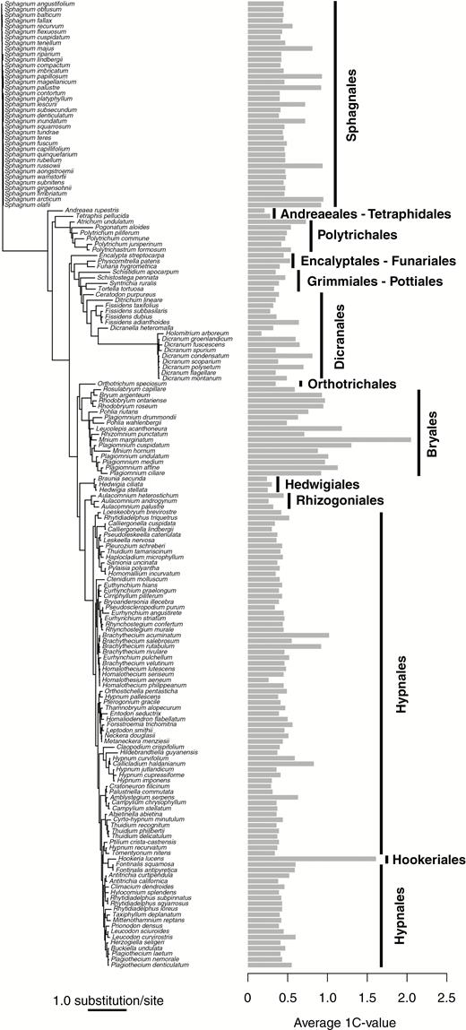
Pruned phylogram of 173 species with the average 1C-values for each species plotted and the moss orders indicated with vertical bars. For species with multiple 1C-values, the smallest value was used as a conservative estimate of genome size.
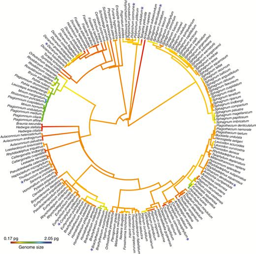
Continuous character state mapping of the average 1C-values, ranging from 0.17 pg (red) to 2.05 pg (blue), onto a pruned ultrametric tree that includes 173 taxa using the ContMap function with default settings from the phytools package in R. For species with multiple 1C-values, the smallest value was used as a conservative estimate of genome size. Species with more than one 1C-value that was approximately double the smallest value are indicated on the phylogeny with a blue asterisk as a potential within-species polyploidization event.
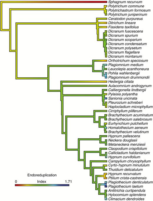
Continuous character state mapping of the endoreduplication index (EI) ranging from 0 (red) to 1.71 (blue) on a pruned ultrametric tree that includes 48 taxa using the ContMap function with default settings from the phytools package in R (Revell, 2012; R Core Team, 2017).
The ancestral character state mapping indicates multiple evolutionary transitions from a very small ancestral genome size to slightly larger genome sizes in some derived lineages (Figs 1 and 2). There are at least four independent transitions to slightly larger genome sizes within the Sphagnales, with potentially one reversal to a smaller genome size in Sphagnum magellanicum. There is one transition in the Polytrichales and a gradual increase to slightly larger genome sizes in the Dicranales (Fig. 2). Members of the Bryales have the largest moss genome sizes, which appears to represent a single transition. This lineage also appears to contain two reversals to smaller genome sizes in Plagiomnium + Pohlia, and Rosulabryum (Fig. 2). On the whole, the Hypnales contain relatively small genomes with the exception of two transitions to slightly larger genome sizes in Brachythecium and Callicladium. The only member sampled from the Hookeriales, Hookeria lucens, has a genome size that is nearly double that of members of the closely related Hypnales. Overall, this analysis reconstructs ten independent increases in genome size across the moss phylogeny and the potential for three reversals (Fig. 2), which calls into question the idea that genome size evolution is unidirectional and does not support the genetic obesity hypothesis (Bennetzen and Kellogg, 1997) for mosses.
Comparative phylogenetic analyses were calculated independently for genome size and EI across the pruned trees. We optimized the value of Pagel’s λ using maximum likelihood with no constraints and compared that with the likelihood of a model where λ was constrained to zero (no phylogenetic signal). Based on likelihood ratio tests, significant phylogenetic signal was detected for genome size (λ = 0.56, logL = 119.92, logL0 = 95.17, P = 1.98e−12), whereas significant phylogenetic signal was not detected for the EI (λ = 6.62e−5, logL = 4.75, logL0 = 4.75, P = 1) across the pruned phylogenies.
The most likely tree for the full dataset was then pruned to include only the taxa for which 1C-values and EI values were available. This resulted in a tree that included 48 moss species. Using the phylogenetically corrected values, which take into account the distance between species, genome size and EI were found to be negatively correlated; however, this relationship was not statistically significant (F1,46 = 1.39, r= −0.31, adjusted r2 = 0.008, P = 0.245).
Overall the vast majority of the mosses sampled have detectable levels of endoreduplication with the exception of the single member of the genus Sphagnum included in this study (Fig. 3). Members of the genera Ditrichum, Orthotrichum, Hedwigia, Hypnum and Ptilidium have lower levels of endoreduplication relative to the ancestral condition, while Plagiomnium, Sanionia and Plagiothecium have higher levels (Fig. 3).
DISCUSSION
This study analysed the most comprehensive dataset of 1C-values and endopolyploidy data assembled to date from a broad phylogenetic sample of moss species. These data do not support the genetic obesity hypothesis (Bennetzen and Kellogg, 1997) for mosses, which postulates that genome size evolution is unidirectional, resulting in species with larger genomes occupying derived positions within the phylogeny. We determined that there is phylogenetic signal for genome size across mosses, which is the tendency of closely related species to resemble each other more than a random set of species from the same tree (Harvey and Pagel, 1991); however, no phylogenetic signal was detected for endopolyploidy. We also did not find a significant correlation between endopolyploidy and genome size across mosses (Nagl, 1978; De Rocher et al., 1990; Barow and Meister, 2003; Bainard et al., 2012), using phylogenetic comparative methods that account for the non-independence of data collected across species (Felsenstein, 1985).
Variation in genome size
Relative to other land plant lineages (Bennett and Leitch, 2012), the diversity of genome size estimates we observed across mosses is significantly smaller (Figs 1 and 2, Table 1, Supplementary Data Table S2), which is in line with previous findings (Reski et al., 1994; Renzaglia et al., 1995; Lamparter et al., 1998; Temsch et al., 1998; Zouhair and Lecocq, 1998; Voglmayr, 2000; Schween et al., 2003; Melosik et al., 2005; Bainard et al., 2010). Thus far, no moss genomes have been found that are larger than 2004 Mbp (Mnium marginatum; Voglmayr, 2000), and in the present study only three species had genomes over 1000 Mbp (Cirriphyllum piliferum, Leucolepis acanthoneura and Polytrichum commune; Table 1). This is similar to hornworts, where all genome size estimates to date are under 500 Mbp (Bainard and Villarreal, 2013) but is in contrast to the liverworts which have many representatives with small genomes, but also several species with 1C-values over 1000 Mbp and one species over 20 000 Mbp (Phyllothallia fuegiana; Bainard et al., 2013). Despite the sister relationship between the moss and liverwort lineages (Puttick et al., 2018; Renzaglia et al., 2018), it appears that the larger genome condition has arisen independently within the liverwort clade and is not a feature shared with mosses. Within mosses, some orders and families demonstrate slightly larger genome sizes compared with others (Fig. 1). For example, the Brachytheciaceae and Mniaceae, which are both in the Bryales, contain a number of species with relatively larger genome sizes, including the species with the largest moss genome size, Mnium marginatum. The Bryales appear to have a considerable number of polyploid occurrences within the order based on chromosome sizes (Fritsch, 1991), which may contribute to the larger genome sizes. The single member of the Hookeriales included in this study also has a slightly larger genome (Hookeria lucens, 1.61 pg; Figs 1 and 2), however, additional samples are needed to confirm this observation throughout the order.
Though the majority of genome size estimates from the same species were equivalent, we also found evidence of intraspecific variation in 1C-values, both within this study and in comparison with previous estimates (Tables 1 and 2). Species that include 1C-values that are approximately double each other may be due to polyploidy (noted with an asterisk in Fig. 2), which is common in mosses, and is thought to occur in as many as 14.3 % of moss species (Såstad, 2005). Once a polyploidization event has occurred (potentially through unreduced spore production or hybridization), a population of diploid gametophytes can be maintained via fragmentation or other forms of asexual reproduction. Aneuploidy, which is a change in chromosome number by less than a complete chromosome set, may also explain intraspecific variation in 1C-values and is suggested to play a major role in bryophyte evolution (Newton, 1984). However, the wide variation in chromosome counts for a single species of mosses (Fritsch, 1991) means that chromosome numbers must be determined from the same sample as the genome size estimates, which could not be determined post hoc for the genome sizes compiled from the literature in this study. It is notable that in two of the mosses analysed here that show possible ploidy variation, Campylium chrysophyllum and Polytrichum commune (Fig. 2), Fritsch (1991) also reports chromosome counts in some accessions that are double that of the rest.
Other variations in the genome size estimates between the present study and Voglmayr (2000) are possibly due to differences in flow cytometry methodology. Specifically, the use of higher PI concentration (150 versus 60 μg mL−1) has been shown to result in higher DNA content estimates (Bainard et al., 2010). All of the estimates that were determined to be different between the present study and Voglmayr (2000), as based on the criterion of a ratiomax/min >1.15, were found to be higher here than those in Voglmayr (2000), excluding differences attributable to a potential variation in ploidy. Voglmayr (2000) also used Baranyi’s buffer, which has a chemical composition different from the LB01 buffer and was found to produce slightly higher 1C-value estimates than LB01 (Bainard et al., 2010).
Across plants, genome size is strongly correlated with the proportion of transposable elements in the genome (Ågren and Wright, 2015). Genomic research on the model moss Physcomitrella patens found that, similar to many other plants, transposable elements make up a considerable portion of the P. patens genome, with ~50 % of the genome consisting of LTR retrotransposons (Rensing et al., 2008). In P. patens, greater accumulation of repetitive DNA may be limited by extremely efficient homologous recombination (Reski, 1998; Schween et al., 2003). Across mosses, high amounts of asexual reproduction might also play a role in the maintenance of a small genome, as transposable elements are unlikely to be maintained (Dolgin and Charlesworth, 2006)
Variation in endopolyploidy
The new estimates determined in this study continue to support the high prevalence of endoreduplication in mosses (Fig. 3, Table 1), except for Sphagnum. Despite the lack of endopolyploidy detected for Sphagnum, this process may play a role in the development of the large hyaline cells that enable these mosses to hold up to 10–25 times their dry weight in water (Andrus, 1986). Transmission electron micrographs of developing hyaline cells show large nuclei compared with nuclei in the surrounding chlorophyllose cells (Kremer and Drinnan, 2004). Detecting endopolyploidy in these cells is impossible at maturity due to disintegration of nuclei and cell death. While our samples for this study were taken from the actively growing apical regions of the Sphagnum gametophytes, the samples may have lacked immature hyaline cells with intact nuclei. Sampling of additional taxa with a focus on large amounts of young, meristematic tissues may increase the likelihood of endopolyploidy detection, if it is present at all in Sphagnum. The apparent lack of endoreduplication in hornworts, liverworts, ferns and gymnosperms suggests that this trait arose independently in mosses and again in specific angiosperm lineages. Additional work is needed to more fully understand the distribution of endopolyploidy across land plants.
Surveys of endopolyploidy across angiosperms found that genome size was negatively correlated with degree of endopolyploidy in broad surveys across taxonomic groups (e.g. Bainard et al., 2012) and in specific families: Brassicaceae, Solanaceae and Urticaceae (Nagl, 1978; Barow and Meister, 2003). Our study includes multiple members from some moss families (i.e. Brachytheciaceae, Dicranaceae, Hypnaceae and Mniaceae); however, our focus on sampling across the breadth of the moss phylogeny did not allow similar tests within families. Despite the lack of correlation between genome size and endopolyploidy across the moss phylogeny, all mosses sampled have small genomes and all were found to be endopolyploid with the exception of Sphagnum. Increased sampling within targeted sets of moss families will enable us to explore this relationship on a similar level in future studies.
Biological significance of DNA content variation in mosses
The amount of DNA in a genome, known as genome size or C value, varies greatly across living organisms and is known to correlate with a number of phenotypic traits, most notably cell size (e.g. Cavalier-Smith, 1978; Gregory, 2001), which in turn has been suggested to impact a variety of other morphological and physiological factors (the nucleotypic theory; Bennett, 1971; ,Bennett, 1972). For example, in angiosperms genome size has been linked with seed size (Beaulieu et al., 2007), stomata size and density (Beaulieu et al., 2008; Hodgson et al., 2010) and primary productivity (Simonin and Roddy, 2018). Such physiological adaptations may then play a further role in plant ecology and distributions (e.g. Knight and Ackerly, 2002; Knight et al., 2005).
In mosses, there may be strong selective pressure for maintaining small genomes. Renzaglia et al. (1995) discovered a strong correlation between sperm cell length and C value in hornworts, liverworts and mosses, providing a possible explanation for the constrained genome sizes. The selective pressures acting on sperm size are expected to be high, as reproductive success relies heavily on sperm locomotion (Renzaglia et al., 1995). Another physiological aspect that might be under selective pressure in mosses is desiccation tolerance. In mosses, cell size appears to be a limiting factor for desiccation tolerance (Proctor et al., 1998), which could then link back to minimum DNA content. Baniaga et al. (2016) also suggested that small genomes may play a role in desiccation tolerance in the Selaginellales and in Genlisea tuberosa.
Biologically, endopolyploidy plays a role in the formation of specialized cells and tissues (Nagl, 1978; Maluszynska et al., 2013), and in mosses occurs in food-conducting cells, mucilagenous hairs and rhizoids (Leitch and Dodsworth, 2017). The fact that these specialized tissues have endopolyploid nuclei suggests a potential functional significance for endoreduplication, including an increase in gene copy number that may lead to increases in gene expression and the ability to produce a range of cell sizes. The highly ubiquitous nature of endopolyploid nuclei in mosses, which is absent in many other early-diverging plant lineages, provides an impetus to study this group in more detail. Targeted approaches with high levels of sampling within particular lineages, such as the Bryales and Hookeriales, will enable us to test explicit hypotheses about the evolution of relatively larger genome sizes in these lineages. Many lineages also showed evidence of polyploidization, and pairing genome size data with chromosome data from the same populations will strengthen our understanding of these patterns. Further exploration of the nucleotypic theory in mosses, specifically focusing on sperm size and desiccation tolerance, may yield unique insights into the evolution of these traits.
SUPPLEMENTARY INFORMATION
Supplementary data are available online at https://dbpia.nl.go.kr/aob and consist of the following. Table S1: voucher specimens of all collected materials deposited in the Biodiversity Institute of Ontario Herbarium. Table S2: genome size data analysed from the literature. Table S3: SUMAC-generated list of the 2214 moss species from 35 families, including GenBank numbers for the four gene regions. Table S4: data set details for individual gene regions and the full data set of 2214 species.
FUNDING
This work was supported by The Natural Sciences and Engineering Research Council of Canada (NSERC) to J.D.B. and to S.G.N, and the Canadian Foundation for Innovation to S.G.N.
ACKNOWLEDGEMENTS
We thank the following people for contributing to specimen collection: A. Garrett, M. Kuzmina, J. Maloles and N. Webster. We value the expert assistance of N. R. Patel with uploading our data to TreeBASE. We greatly appreciate comments from P. Kron and anonymous reviewers on earlier versions of this manuscript.
