


Abstract
Measurement error is common in epidemiology, but few studies use quantitative methods to account for bias due to mismeasurement. One potential barrier is that some intuitive approaches that readily combine with methods to account for other sources of bias, like multiple imputation for measurement error (MIME), rely on internal validation data, which are rarely available. Here, we present a reparameterized imputation approach for measurement error (RIME) that can be used with internal or external validation data. We illustrate the advantages of RIME over a naive approach that ignores measurement error and MIME using a hypothetical example and a series of simulation experiments. In both the example and simulations, we combine MIME and RIME with inverse probability weighting to account for confounding when estimating hazard ratios and counterfactual risk functions. MIME and RIME performed similarly when rich external validation data were available and the prevalence of exposure did not vary between the main study and the validation data. However, RIME outperformed MIME when validation data included only true and mismeasured versions of the exposure or when exposure prevalence differed between the data sources. RIME allows investigators to leverage external validation data to account for measurement error in a wide range of scenarios.
Abbreviations
- ESRD
end-stage renal disease
- CI
confidence interval
- GFR
glomerular filtration rate
- MIME
multiple imputation for measurement error
- RIME
reparameterized imputation for measurement error
Exposure measurement error is an important and common threat to the validity of epidemiologic studies. Multiple imputation for measurement error (MIME) is a valid approach to account for exposure measurement error in some settings and is appealing because it can be used in concert with almost any approach for data analysis, including settings with measured confounding and informative censoring (1, 2). Moreover, MIME draws on methods for handling missing data that are familiar to many epidemiologists (3, 4). However, existing work describing multiple imputation to account for exposure measurement error is limited to settings with internal validation data.
Although the use of internal validation data is generally preferred to external validation data when correcting for measurement error, using internal validation data is often infeasible given the logistics and cost associated with collecting this information. Moreover, secondary data analysis or analysis of data others have collected might not allow opportunities for internal validation studies.
MIME relies on internal validation data because it models the predictive values directly. In 2006, Cole, Chu, and Greenland (1) noted that one could reparameterize MIME by modeling sensitivity and specificity rather than the predictive values. Here, we show that this reparameterization enables the use of imputation approaches to account for exposure measurement error in settings without internal validation data but with some knowledge of the misclassification probabilities (from an external validation study or prior knowledge). The proposed approach, which we refer to as “reparameterized imputation for measurement error” (RIME), relaxes the strict assumption that the positive and negative predictive values are transportable between the main study and the validation sample and instead relies only on transportability of sensitivity and specificity. When an internal validation study is conducted among a random sample of main study participants, we expect MIME and RIME to yield equivalent results. However, in settings with only external validation data or a biased internal validation sample, we expect RIME to outperform MIME.
We illustrate use of the new, reparameterized imputation for measurement error correction using the same hypothetical study of the effect of low glomerular filtration rate on end-stage renal disease (ESRD) used by Cole, Chu, and Greenland (1), and we explore finite sample properties of the proposed approach using a series of simulation experiments.
METHODS
Hypothetical cohort
We first illustrate the proposed reparameterized imputation approach using the hypothetical study population described by Cole, Chu, and Greenland (1), with slight modification. Briefly, the data set contains records for 600 children between the ages of 1 and 16 years with chronic kidney disease, and the parameter of interest is the effect on ESRD of low glomerular filtration rate (GFR) at study entry relative to moderate GFR. We present both the hazard ratio for the effect of low GFR and the risk difference comparing risk of ESRD at 3 years between the groups. We extend the data set described by Cole, Chu, and Greenland (1) to include binary confounder |$L$|, which affects both GFR and ESRD. Let participants be indexed by |$i$|; |${T}_i$| represents the time from study entry until ESRD, |${X}_i$| represents true GFR level (low vs. moderate), and |${W}_i$| represents measured GFR level. Because some individuals are censored at time |${C}_i$|, let |${Y}_i=\min \big({T}_i,{C}_i\big)$| and |${\delta}_i$| represent an indicator that the individual had the event prior to |${C}_i$|. The index |$i$| will be suppressed where possible below for clarity. Assume that |$Y,\delta$|, and |$L$| are measured without error in the hypothetical data. Although the data set contains both the true GFR status |$X$| and the possibly mismeasured GFR status |$W$|, we assume that only |$W$| is observed in the main study data.
Finally, we generated 2 separate external validation data sets composed of 150 records not included in the main study. The first external validation data set included only information on measured GFR |$W$| and gold-standard GFR measurement |$X$|. The second validation data set included information on outcomes |$Y$| and |$\delta$| and covariate |$L$| in addition to |$W$| and |$X$|. In both validation data sets, the prevalence of true exposure |$X$| was the same as in the main study, although we later explore a set of scenarios in simulations in which the prevalence of |$X$| in external validation data set 2 ranged from 25% to 90%. Details of the data-generating mechanisms for both hypothetical data sets and the external validation data set are available in Web Appendix 1 (available at https://dbpia.nl.go.kr/aje).
Analysis of the hypothetical cohort
We estimated standardized hazard ratios and risk differences for the effect of GFR on ESRD accounting for confounding by |$L$| in the hypothetical cohort using 3 analytical approaches to account for exposure misclassification: a naive approach, the traditional multiple imputation approach to account for measurement error (MIME), and the proposed approach (RIME). Each of these approaches was compared with the “full data” approach, which used data on the true, but usually unobserved, exposure |$X$|.
Full data
The first parameter of interest was the hazard ratio for the effect of GFR on ESRD corresponding to |$\exp \big(\alpha \big)$| from the marginal structural Cox model |${h}_{T^x}(t)={h}_0(t)\mathit{\exp}\big\{\alpha x\big\}$|, where |${T}^x$| represents the time from study entry until ESRD under exposure |$x$|. Using the full data, we estimated this hazard ratio as |$\exp \big(\hat{\alpha}\big)$|, where |$\hat{\alpha}$| was estimated by maximizing the weighted partial likelihood:
The second parameter of interest was the risk difference under low versus moderate GFR at 3 years after study entry. We defined risk under each GFR level as |${F}_{T^x}(t)=P({T}^x\le t)$| (7). In the full data, we estimated the risk under each exposure as the complement of the weighted Kaplan-Meier (8) estimate of the survival function at 3 years. Specifically, the risk function for exposure group |$X=x$| was estimated as |${\hat{F}}_{T^x}(t)=1-{\prod}_{t_{j}\le t}\big\{1-{d}_{t_{j},x}^{\pi}/{n}_{t_{j},x}^{\pi}\big\}$|, where |${d}_{t_{j},x}^{\pi}$| and |${n}_{t_{j},x}^{\pi}$| were the weighted number of events and number in the risk set at event time |${t}_j$| for participants with |$X=x$|, respectively. Confidence intervals around the risk difference were constructed as plus or minus 1.96 times the standard error, where the standard error was estimated as the standard deviation of the risk difference in 1,000 bootstrap samples of the main study data.
Standard approach
Because, in real-world scenarios, the true exposure is unobserved, the “standard approach” estimated the parameters of interest using the possibly mismeasured exposure |$W$| in place of |$X$|. Specifically, we estimated the hazard ratio as |$\exp (\hat{\alpha}^{\prime})$|, where |$\hat{\alpha}^{\prime }$| was estimated by maximizing the weighted partial likelihood:
Multiple imputation for measurement error
The traditional MIME approach was based on modeling the predictive values in the validation sample as described by Cole, Chu, and Greenland (1) and elsewhere (as in Edwards et al. (9)). We implemented MIME to account for exposure measurement error in the hazard ratio and risk difference, first using external validation data set 1 and then using external validation data set 2. Briefly, this approach required: 1) fitting an imputation model for the exposure in the validation data set to obtain estimates of the “predictive values,” or the probability that each participant in the validation data set was truly exposed given available variables; 2) imputing the true exposure |$k$| times for participants in the main study data using the predictive values; 3) conducting the analyses in each imputed data set; and 4) combining results across imputations using standard multiple imputation techniques (10). Confidence intervals around hazard ratios were constructed using Rubin’s Rules (10), which combine within-imputation variability (conveyed by the robust standard error estimated in each imputation) and between-imputation variability, while confidence intervals around risk differences were constructed using the nonparametric bootstrap.
Literature on MIME suggests including outcomes and covariates used in the weights in the imputation model. However, when using external validation data, these variables are frequently unavailable. Accordingly, we first implemented MIME using only the information contained in external validation data set 1, which included measurements on |$X$| and |$W$| only. Using external data set 1, we predicted the probability of |$X$| in the validation data conditional on |$W$| using logistic regression: |$P(X=1|W)=\mathrm{expit}\{{\beta}_0+{\beta}_1W\}$|. We used information on |${\hat{\beta}}_0$| and |${\hat{\beta}}_1$| and values of |$W$| in the main study to impute |${X}^k$| for all participants in the main study for each of |$K$| imputations, indexed by |$k$|.
Example Data for 600 Children With Chronic Kidney Disease
| True GFR Status | Overall | |||||
|---|---|---|---|---|---|---|
| Moderate: X |$=\mathbf{0}\ $|(n |$ =\mathbf{359}$|) | Low: X |$=\mathbf{1} $|(n |$ =\mathbf{241}$|) | (n |$=\mathbf{600}$|) | ||||
| Characteristic | No. | % | No. | % | No. | % |
| Measured GFR status | ||||||
| |$W=0$| | 251 | 69.9 | 23 | 9.5 | 274 | 45.7 |
| |$W=1$| | 108 | 30.1 | 218 | 90.5 | 326 | 54.3 |
| Confounder | ||||||
| |$L=0$| | 120 | 33.4 | 177 | 73.4 | 300 | 50.0 |
| |$L=1$| | 239 | 66.6 | 61 | 25.3 | 300 | 50.0 |
| Events | 70 | 19.5 | 64 | 26.6 | 134 | 22.3 |
| Total no. of person-years | 997 | 650 | 1,647 | |||
Abbreviations: GFR, glomerular filtration rate; L, binary confounder; W, study measurement of GFR status; X, gold-standard measurement of GFR status.
We next implemented MIME using external validation data set 2, which included information on outcomes and covariates in addition to |$X$| and |$W$|. When using external validation data set 2, we fit the imputation model |$P(X=1|W,Y,\delta, L)=\mathrm{expit}\{{\beta}_0+{\beta}_1W+{\beta}_2\log (Y)+{\beta}_3\delta +{\beta}_4L\}$| and used estimated values of |${\beta}_1$| through |${\beta}_4$| along with values of |$\{W,Y,\delta, L\}$| in the main study to impute |${X}^k$|.
Analyses (e.g., weighted Cox models and estimation of risk functions) were implemented in each imputed data set and results were combined across imputations using standard multiple imputation techniques. Details about implementation of the MIME approach are provided in Web Appendix 2.
Example Validation Data Set 1a to Validate Glomerular Filtration Rate Status Among Children With Chronic Kidney Disease
| X |$=\mathbf{0}$| | X |$=\mathbf{1}$| | |
|---|---|---|
| |$W=0$| | 62 | 5 |
| |$W=1$| | 27 | 56 |
| X |$=\mathbf{0}$| | X |$=\mathbf{1}$| | |
|---|---|---|
| |$W=0$| | 62 | 5 |
| |$W=1$| | 27 | 56 |
Abbreviations: GFR, glomerular filtration rate; W, study measurement of GFR status; X, gold-standard measurement of GFR status.
a Contains records for 150 participants not included in the main study. Contains information on W and X only for all participants. Overall prevalence of X is about the same as in the main study.
Reparameterized imputation for measurement error
Like MIME, the proposed reparameterized imputation approach (RIME) relied on accurately estimating the “predictive values,” or the probability that each participant was exposed, given his or her observed exposure and outcome. Let |${\omega}_i$| represent the predictive value |${\omega}_i=P(X=1|W_i,\delta_i, \log \{Y_i\},L_i)$|. Unlike MIME, RIME did not estimate the predictive values directly from the validation sample; instead, we used the external validation data set to estimate sensitivity |$(\mathrm{se}=P(W=1|X=1))$| and specificity |$(\mathrm{sp}=P(W=0|X=0))$|. To estimate the predictive values in the main study, we applied Bayes’ theorem:
Confidence intervals for the hazard ratios and risk differences estimated using RIME were constructed as the point estimate (i.e., risk difference or log(hazard ratio)) plus or minus 1.96 times the standard deviation of the point estimate from 1,000 bootstrap samples of the main study and validation data. Specifically, in each bootstrap iteration |$q$|, sensitivity |${\hat{\mathrm{se}}}_q$| and specificity |${\hat{\mathrm{sp}}}_q$| were estimated from the resampled external validation data, the modified likelihood function was fit in the resampled main study data to estimate |${\hat{\mu}}_q$|, and |${\hat{\mu}}_q$| was combined with estimated |${\hat{\mathrm{se}}}_q$| and |${\hat{\mathrm{sp}}}_q$| to estimate |${\hat{\omega}}_{i,q}$| and determine the misclassification weights for that iteration.
R (R Foundation for Statistical Computing, Vienna, Austria) code to implement RIME to obtain hazard ratios in the example data is provided in Web Appendix 4.
Simulations
To examine the finite sample properties of the proposed approach, we repeated the hypothetical study described above 1,000 times and summarized the results under several values of sensitivity and specificity and under various sizes of the external validation data set. We compared the performance of the naive approach, MIME, and RIME to estimate both hazard ratios and risk differences, where MIME and RIME were implemented using external validation data set 1 or external validation data set 2. Specifically, we compared bias, standard error, root mean squared error, and 95% confidence interval coverage probabilities among the 3 approaches. When estimating the hazard ratio, bias was defined as the difference between the true log hazard ratio and the estimated log hazard ratio. When estimating the risk difference, bias was defined as 100 times the difference between the true risk difference and the estimated risk difference. Standard errors were computed as the average estimated standard error for the log hazard ratio or risk difference over all trials. Root mean squared error was the square root of the sum of the squared bias and the variance. Finally, 95% coverage probability was the proportion of simulated studies in which the 95% confidence interval contained the true parameter value.
Example Validation Data Set 2a to Validate Glomerular Filtration Rate Status Among Children With Chronic Kidney Disease
| X |$=\mathbf{0}$| | X |$=\mathbf{1}$| | |
|---|---|---|
| |$W=0$| | 62 | 5 |
| |$W=1$| | 27 | 56 |
| |$L=0$| | 30 | 45 |
| |$L=1$| | 59 | 16 |
| No. of events | 29 | 18 |
| No. of person-years | 232 | 163 |
| X |$=\mathbf{0}$| | X |$=\mathbf{1}$| | |
|---|---|---|
| |$W=0$| | 62 | 5 |
| |$W=1$| | 27 | 56 |
| |$L=0$| | 30 | 45 |
| |$L=1$| | 59 | 16 |
| No. of events | 29 | 18 |
| No. of person-years | 232 | 163 |
Abbreviations: GFR, glomerular filtration rate; L, binary confounder; W, study measurement of GFR status; X, gold-standard measurement of GFR status.
a Contains records for 150 participants not included in the main study. Contains information on W, X, L events and person-years for all participants. Overall prevalence of X is about the same as in the main study.
Comparing Incidence of End-Stage Renal Disease Between Children With Low Glomerular Filtration Rate and Children With Moderate Glomerular Filtration Rate From a Hypothetical Cohort Study of 600 Children
| Weighted Hazard Ratios | 3-Year Risk Differences | |||||
|---|---|---|---|---|---|---|
| Approach | HR | SE for Ln(HR) | 95% CI for HR | RD, % | SE for RD | 95% CI for RD |
| Full data | 2.24 | 0.17 | 1.60, 3.13 | 17.0 | 3.5 | 10.1, 23.9 |
| Naive approach | 1.58 | 0.18 | 1.11, 2.26 | 8.8 | 3.3 | 2.4, 15.2 |
| Using external validation data set 1a | ||||||
| MIME | 1.30 | 0.11 | 1.06, 1.61 | 5.3 | 2.1 | 1.1,9.5 |
| RIME | 2.19 | 0.32 | 1.17, 4.11 | 16.1 | 7.7 | 1.0, 31.0 |
| Using external validation data set 2b | ||||||
| MIME | 2.74 | 0.30 | 1.53, 4.90 | 21.7 | 6.6 | 8.8, 34.6 |
| RIME | 2.19 | 0.33 | 1.15, 4.15 | 16.1 | 7.9 | 0.7, 31.5 |
Abbreviations: CI, confidence interval; GFR, glomerular filtration rate; HR, hazard ratio; MIME, multiple imputation for measurement error; RD, risk difference; RIME, reparametrized imputation for measurement error; SE, standard error.
a External validation data set 1 contains data on true and error-prone measurements of GFR among 150 children recruited from outside the main study.
b External validation data set 2 contains data on true and error-prone measurements of GFR, binary confounder L, and outcomes among 150 children recruited from outside the main study.
Next, we examined the robustness of MIME and RIME to the prevalence of exposure in the external validation sample. In the scenario in which sensitivity was 0.9 and specificity was 0.7 using external validation data set 2, we compared the naive approach, MIME, and RIME under varying prevalence of true exposure in the validation data set. As in the hypothetical studies and simulations described above, the true, but unobserved, exposure prevalence in the main study was 40%. We varied the prevalence of the true exposure in the validation study from 25% to 90% in increments of 5% and calculated the bias for each approach under each scenario.
| Naive | MIME | RIME | ||||||||||
|---|---|---|---|---|---|---|---|---|---|---|---|---|
| Sensitivity, Specificity, and nvf | Bias | SE | RMSE | Cover | Bias | SE | RMSE | Cover | Bias | SE | RMSE | Cover |
| External Validation Data Set 1 | ||||||||||||
| 0.9, 0.9 | ||||||||||||
| 150 | −0.21 | 0.17 | 0.27 | 0.75 | −0.34 | 0.14 | 0.37 | 0.29 | 0.00 | 0.26 | 0.26 | 0.94 |
| 300 | −0.21 | 0.17 | 0.27 | 0.75 | −0.35 | 0.13 | 0.37 | 0.26 | 0.00 | 0.25 | 0.25 | 0.95 |
| 0.9, 0.7 | ||||||||||||
| 150 | −0.38 | 0.17 | 0.42 | 0.38 | −0.55 | 0.10 | 0.56 | 0.00 | −0.01 | 0.37 | 0.37 | 0.95 |
| 300 | −0.38 | 0.17 | 0.42 | 0.38 | −0.55 | 0.10 | 0.56 | 0.00 | −0.01 | 0.36 | 0.36 | 0.94 |
| 0.7, 0.9 | ||||||||||||
| 150 | −0.34 | 0.17 | 0.38 | 0.50 | −0.52 | 0.11 | 0.53 | 0.01 | −0.01 | 0.36 | 0.36 | 0.96 |
| 300 | −0.34 | 0.17 | 0.38 | 0.50 | −0.53 | 0.10 | 0.54 | 0.00 | 0.00 | 0.34 | 0.34 | 0.96 |
| 0.7, 0.7 | ||||||||||||
| 150 | −0.52 | 0.17 | 0.55 | 0.11 | −0.67 | 0.07 | 0.68 | 0.00 | −0.04 | 0.62 | 0.62 | 0.97 |
| 300 | −0.52 | 0.17 | 0.55 | 0.11 | −0.67 | 0.07 | 0.68 | 0.00 | −0.02 | 0.60 | 0.60 | 0.97 |
| External Validation Data Set 2 | ||||||||||||
| 0.9, 0.9 | ||||||||||||
| 150 | −0.21 | 0.17 | 0.27 | 0.75 | −0.02 | 0.27 | 0.27 | 0.96 | 0.00 | 0.26 | 0.26 | 0.94 |
| 300 | −0.21 | 0.17 | 0.27 | 0.75 | −0.01 | 0.20 | 0.20 | 0.96 | 0.00 | 0.25 | 0.25 | 0.95 |
| 0.9, 0.7 | ||||||||||||
| 150 | −0.38 | 0.17 | 0.42 | 0.38 | −0.02 | 0.30 | 0.30 | 0.97 | −0.01 | 0.37 | 0.37 | 0.95 |
| 300 | −0.38 | 0.17 | 0.42 | 0.38 | −0.01 | 0.21 | 0.21 | 0.96 | −0.01 | 0.36 | 0.36 | 0.94 |
| 0.7, 0.9 | ||||||||||||
| 150 | −0.34 | 0.17 | 0.38 | 0.50 | 0.00 | 0.31 | 0.31 | 0.95 | −0.01 | 0.36 | 0.36 | 0.96 |
| 300 | −0.34 | 0.17 | 0.38 | 0.50 | 0.01 | 0.22 | 0.22 | 0.97 | 0.00 | 0.34 | 0.34 | 0.96 |
| 0.7, 0.7 | ||||||||||||
| 150 | −0.52 | 0.17 | 0.55 | 0.11 | 0.01 | 0.34 | 0.34 | 0.95 | −0.04 | 0.62 | 0.62 | 0.97 |
| 300 | −0.52 | 0.17 | 0.55 | 0.11 | 0.02 | 0.23 | 0.23 | 0.97 | −0.02 | 0.59 | 0.59 | 0.96 |
Abbreviations: HR, hazard ratio; MIME, multiple imputation for measurement error; RIME, reparametrized imputation for measurement error; RMSE, root mean squared error; SE, standard error.
a Bias was defined as the difference between the true ln(HR) and the estimated ln(HR).
b Standard error was defined as the average standard error over all simulated cohorts. For the RIME approaches, standard errors for the hazard ratios were estimated as the standard deviation of the ln(HR) in 1,000 bootstrap samples of each simulated data set.
c RMSE was the square root of the bias squared plus the variance.
d 95% confidence interval coverage was the proportion of simulated data sets in which the estimated 95% confidence interval contained the true value.
e Scenarios varying the type of validation data available, sensitivity, specificity, and the size of the validation study.
f nv represents the size of the external validation study.
| Naive | MIME | RIME | ||||||||||
|---|---|---|---|---|---|---|---|---|---|---|---|---|
| Sensitivity, Specificity, and nvf | Bias | SE | RMSE | Cover | Bias | SE | RMSE | Cover | Bias | SE | RMSE | Cover |
| External Validation Data Set 1 | ||||||||||||
| 0.9, 0.9 | ||||||||||||
| 150 | −0.21 | 0.17 | 0.27 | 0.75 | −0.34 | 0.14 | 0.37 | 0.29 | 0.00 | 0.26 | 0.26 | 0.94 |
| 300 | −0.21 | 0.17 | 0.27 | 0.75 | −0.35 | 0.13 | 0.37 | 0.26 | 0.00 | 0.25 | 0.25 | 0.95 |
| 0.9, 0.7 | ||||||||||||
| 150 | −0.38 | 0.17 | 0.42 | 0.38 | −0.55 | 0.10 | 0.56 | 0.00 | −0.01 | 0.37 | 0.37 | 0.95 |
| 300 | −0.38 | 0.17 | 0.42 | 0.38 | −0.55 | 0.10 | 0.56 | 0.00 | −0.01 | 0.36 | 0.36 | 0.94 |
| 0.7, 0.9 | ||||||||||||
| 150 | −0.34 | 0.17 | 0.38 | 0.50 | −0.52 | 0.11 | 0.53 | 0.01 | −0.01 | 0.36 | 0.36 | 0.96 |
| 300 | −0.34 | 0.17 | 0.38 | 0.50 | −0.53 | 0.10 | 0.54 | 0.00 | 0.00 | 0.34 | 0.34 | 0.96 |
| 0.7, 0.7 | ||||||||||||
| 150 | −0.52 | 0.17 | 0.55 | 0.11 | −0.67 | 0.07 | 0.68 | 0.00 | −0.04 | 0.62 | 0.62 | 0.97 |
| 300 | −0.52 | 0.17 | 0.55 | 0.11 | −0.67 | 0.07 | 0.68 | 0.00 | −0.02 | 0.60 | 0.60 | 0.97 |
| External Validation Data Set 2 | ||||||||||||
| 0.9, 0.9 | ||||||||||||
| 150 | −0.21 | 0.17 | 0.27 | 0.75 | −0.02 | 0.27 | 0.27 | 0.96 | 0.00 | 0.26 | 0.26 | 0.94 |
| 300 | −0.21 | 0.17 | 0.27 | 0.75 | −0.01 | 0.20 | 0.20 | 0.96 | 0.00 | 0.25 | 0.25 | 0.95 |
| 0.9, 0.7 | ||||||||||||
| 150 | −0.38 | 0.17 | 0.42 | 0.38 | −0.02 | 0.30 | 0.30 | 0.97 | −0.01 | 0.37 | 0.37 | 0.95 |
| 300 | −0.38 | 0.17 | 0.42 | 0.38 | −0.01 | 0.21 | 0.21 | 0.96 | −0.01 | 0.36 | 0.36 | 0.94 |
| 0.7, 0.9 | ||||||||||||
| 150 | −0.34 | 0.17 | 0.38 | 0.50 | 0.00 | 0.31 | 0.31 | 0.95 | −0.01 | 0.36 | 0.36 | 0.96 |
| 300 | −0.34 | 0.17 | 0.38 | 0.50 | 0.01 | 0.22 | 0.22 | 0.97 | 0.00 | 0.34 | 0.34 | 0.96 |
| 0.7, 0.7 | ||||||||||||
| 150 | −0.52 | 0.17 | 0.55 | 0.11 | 0.01 | 0.34 | 0.34 | 0.95 | −0.04 | 0.62 | 0.62 | 0.97 |
| 300 | −0.52 | 0.17 | 0.55 | 0.11 | 0.02 | 0.23 | 0.23 | 0.97 | −0.02 | 0.59 | 0.59 | 0.96 |
Abbreviations: HR, hazard ratio; MIME, multiple imputation for measurement error; RIME, reparametrized imputation for measurement error; RMSE, root mean squared error; SE, standard error.
a Bias was defined as the difference between the true ln(HR) and the estimated ln(HR).
b Standard error was defined as the average standard error over all simulated cohorts. For the RIME approaches, standard errors for the hazard ratios were estimated as the standard deviation of the ln(HR) in 1,000 bootstrap samples of each simulated data set.
c RMSE was the square root of the bias squared plus the variance.
d 95% confidence interval coverage was the proportion of simulated data sets in which the estimated 95% confidence interval contained the true value.
e Scenarios varying the type of validation data available, sensitivity, specificity, and the size of the validation study.
f nv represents the size of the external validation study.
| Sensitivity, Specificity, and nvf | Naive | MIME | RIME | |||||||||
|---|---|---|---|---|---|---|---|---|---|---|---|---|
| Bias | SE | RMSE | Cover | Bias | SE | RMSE | Cover | Bias | SE | RMSE | Cover | |
| External Validation Data Set 1 | ||||||||||||
| 0.9, 0.9 | ||||||||||||
| 150 | −5.28 | 3.53 | 6.35 | 0.65 | −7.97 | 2.99 | 8.51 | 0.24 | −0.57 | 5.97 | 6.00 | 0.94 |
| 300 | −5.28 | 3.53 | 6.35 | 0.64 | −8.09 | 2.90 | 8.60 | 0.22 | −0.55 | 5.78 | 5.81 | 0.94 |
| 0.9, 0.7 | ||||||||||||
| 150 | −9.19 | 3.45 | 9.82 | 0.26 | −12.32 | 2.14 | 12.51 | 0.00 | −0.75 | 8.43 | 8.46 | 0.92 |
| 300 | −9.19 | 3.46 | 9.82 | 0.26 | −12.39 | 2.07 | 12.56 | 0.00 | −0.62 | 8.16 | 8.18 | 0.94 |
| 0.7, 0.9 | ||||||||||||
| 150 | −7.51 | 3.70 | 8.37 | 0.49 | −11.82 | 2.28 | 12.04 | 0.01 | −0.69 | 7.95 | 7.98 | 0.93 |
| 300 | −7.51 | 3.70 | 8.37 | 0.49 | −11.89 | 2.19 | 12.09 | 0.00 | −0.63 | 7.72 | 7.74 | 0.95 |
| 0.7, 0.7 | ||||||||||||
| 150 | −12.27 | 3.49 | 12.76 | 0.05 | −15.39 | 1.46 | 15.46 | 0.00 | −1.08 | 12.65 | 12.70 | 0.97 |
| 300 | −12.27 | 3.47 | 12.75 | 0.05 | −15.43 | 1.38 | 15.49 | 0.00 | −0.51 | 12.26 | 12.27 | 0.94 |
| External Validation Data Set 2 | ||||||||||||
| 0.9, 0.9 | ||||||||||||
| 150 | −5.28 | 3.53 | 6.35 | 0.65 | −1.57 | 5.55 | 5.76 | 0.95 | −0.57 | 5.96 | 5.98 | 0.94 |
| 300 | −5.28 | 3.53 | 6.35 | 0.64 | −1.28 | 4.33 | 4.52 | 0.94 | −0.55 | 5.76 | 5.78 | 0.95 |
| 0.9, 0.7 | ||||||||||||
| 150 | −9.19 | 3.45 | 9.82 | 0.26 | −1.81 | 6.23 | 6.48 | 0.95 | −0.75 | 8.41 | 8.44 | 0.93 |
| 300 | −9.19 | 3.46 | 9.82 | 0.26 | −1.36 | 4.55 | 4.75 | 0.95 | −0.62 | 8.14 | 8.16 | 0.94 |
| 0.7, 0.9 | ||||||||||||
| 150 | −7.51 | 3.70 | 8.37 | 0.49 | −1.22 | 6.33 | 6.45 | 0.93 | −0.69 | 7.95 | 7.98 | 0.93 |
| 300 | −7.51 | 3.70 | 8.37 | 0.49 | −0.96 | 4.68 | 4.78 | 0.97 | −0.63 | 7.70 | 7.72 | 0.94 |
| 0.7, 0.7 | ||||||||||||
| 150 | −12.27 | 3.49 | 12.76 | 0.05 | −1.20 | 6.78 | 6.88 | 0.94 | −1.08 | 12.66 | 12.71 | 0.96 |
| 300 | −12.27 | 3.47 | 12.75 | 0.05 | −0.77 | 4.88 | 4.94 | 0.98 | −0.51 | 12.28 | 12.29 | 0.94 |
Abbreviations: MIME, multiple imputation for measurement error; RIME, reparametrized imputation for measurement error; RMSE, root mean squared error; SE, standard error.
a Bias was defined as the difference between the true risk difference and the estimated risk difference.
b Standard error was defined as the average standard error over all simulated cohorts. For all approaches, standard errors were estimated as the standard deviation of the risk difference in 1,000 bootstrap samples of each simulated data set.
c RMSE was the square root of the bias squared plus the variance.
d 95% confidence interval coverage was the proportion of simulated data sets in which the estimated 95% confidence interval contained the true value.
e Scenarios varying the type of validation data available, sensitivity, specificity, and the size of the validation study.
f nv represents the size of the external validation study.
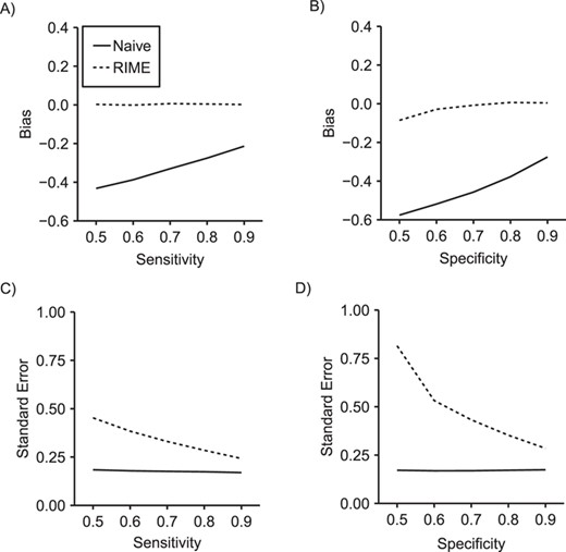
Comparison of bias (panels A and B) and standard error (panels C and D) in the ln(hazard ratio) between reparameterized imputation for measurement error (RIME) and the naive approach as sensitivity varies from 0.5 to 0.9 while specificity is fixed at 0.8 (panels A and C) and as specificity varies from 0.5 to 0.9 while sensitivity is fixed at 0.8 (panels B and D) in 2,000 simulated data sets of size |$n=600$| with an external validation data set of size |${n}_{\mathrm{val}}=150$|.
RESULTS
Hypothetical cohort
Example data for the 600 children in a single draw of the simulated hypothetical cohort are shown in Table 1. Approximately 40% of children in the hypothetical cohort had low GFR, and 50% had confounder |$L$|. In the hypothetical cohort, we assumed that true GFR status |$X$| was unobserved and that we had measured |$W$| in its place. Using the complete data from Table 1, we estimated that the sensitivity of |$W$| as a measure of |$X$| was 90% and its specificity was 70%. By the end of the 3-year study period, 134 ESRD events occurred and children contributed a total of 1,647 person years of follow-up.
External validation data set 1 contained information on |$X$| and |$W$| for a group of 150 participants not included in the main study (Table 2). While the data-generating mechanism dictated that the expected value of sensitivity and specificity in the validation data were the same as in the main study, in this data set, sensitivity of |$W$| as a proxy for |$X$| was 92% and specificity was 70%. External validation data set 2 was identical to external validation data set 1 except that confounder |$L$| and outcomes |$Y$| and |$\delta$| were measured in addition to |$W$| and |$X$| (Table 3).
The 3-year estimated hazard ratio for the effect of low versus moderate GFR, based on the true, but unobserved, GFR measure |$X$| (the “full data” approach), was 2.24 (95% confidence interval (CI): 1.60, 3.13), and the risk difference was 17.0% (95% CI: 10.1, 23.9) (Table 4). When |$W$| was used in place of |$X$| in the “standard” approach, the estimated hazard ratio was 1.58 (95% CI: 1.11, 2.26) and the estimated risk difference was 8.8% (95% CI: 2.4, 15.2). When using external validation data set 1 to account for the exposure misclassification, MIME produced results farther from the full data results than the naive approach (hazard ratio = 1.30, 95% CI: 1.06, 1.61; risk difference = 5.3%, 95% CI: 1.1, 9.5), while RIME produced results near estimates from the full-data approach (hazard ratio = 2.19, 95% CI: 1.17, 4.11; risk difference = 16.1%, 95% CI: 1.0, 31.0). When using external validation data set 2 to account for exposure misclassification, both MIME and RIME produced results similar to each other and near the estimates from the full data approach.
Simulations
Over 1,000 repetitions of the hypothetical study described above, the naive approach produced biased 3-year hazard ratios (Table 5) and risk differences (Table 6), with bias increasing as sensitivity and specificity decreased. When external validation data for each simulated data set were generated using the same data-generating mechanism as external validation data set 1, using MIME produced results with substantial bias and low coverage probability. In contrast, using RIME in conjunction with the same validation data produced results with little bias and appropriate confidence interval coverage. Figure 1 illustrates that RIME produced results with little bias in settings with sensitivity and specificity ranging from 0.5 to 1.0, although precision was reduced for RIME compared with the naive approach, particularly when sensitivity or specificity was low.
When external validation data for each simulated data set were generated using the same data-generating mechanism as external validation data set 2, RIME and MIME both produced results with small bias and appropriate coverage. In this setting, RMSE was slightly smaller for MIME than for RIME. However, when we varied the prevalence of exposure in the external validation data set from 0.25 to 0.9, we saw that MIME was sensitive to discrepancies in exposure prevalence between the main study and external data, while RIME was robust to these differences (Figure 2).
In Web Tables 1 and 2, we provide an additional set of simulation results illustrating that RIME and MIME provide nearly identical results in terms of bias and precision when internal validation data randomly sampled from the main study are available.
DISCUSSION
We have illustrated RIME to account for exposure misclassification in inverse-probability-weighted hazard ratios and risk functions. Using simulations, we showed that RIME provides estimates of the hazard ratio and risk difference with little bias when using external validation data that provides only information on gold-standard and possibly mismeasured exposure. Moreover, even when rich external validation data are available in which outcomes and other covariates are provided, RIME outperforms MIME when the true exposure prevalence in the validation data differs from that in the main study, conditional on other measured variables.
The primary advantage of RIME over MIME is that RIME does not require transportability of the predictive values between the validation data and the main study data. Rather, RIME requires the weaker assumption that sensitivity and specificity are transportable between the data sets. Transportability of sensitivity and specificity is often believed to be a more reasonable assumption than transportability of the predictive values because sensitivity and specificity are properties of the exposure measurement process, while the predictive values are functions of sensitivity, specificity, and the prevalence of true exposure (Rothman et al. (13, p. 355)).
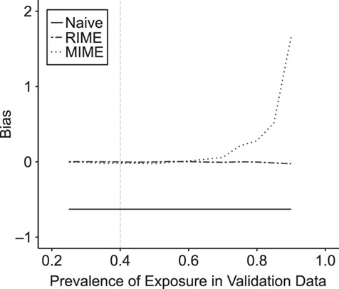
Bias in the estimated inverse probability weighted log(hazard ratio) using the standard approach, multiple imputation for measurement error (MIME), and reparameterized imputation for measurement error (RIME) in settings where external validation data similar to external validation data set 2 are available, but the exposure prevalence in the validation data differs from the exposure prevalence in the main study (shown by vertical gray dashed line).
The proposed RIME approach can be seen as an adaptation of predictive value weighting to account for measurement error. Predictive value weighting for exposure misclassification (14) or outcome misclassification (15) is appealing because it combines easily with analytical approaches to address bias due to other sources, including confounding and selection bias.
Because using RIME in conjunction with inverse probability weights requires multiplying the |$m$|-weight by the inverse probability weight, this approach could result in more extreme weight values. However, because the |$m$|-weights sum to 1 for all of the records contributed by each individual, their use should not alter the mean of the inverse probability weights. Moreover, because inverse probability weights are estimated in the expanded data weighted by the |$m$|-weights, they are likely to be more stable than standard inverse probability weights because all individuals contribute to both exposed and unexposed groups with some probability.
Like RIME, the previously described MIME approach was straightforward to combine with inverse probability of exposure weights to account for confounding. However, unlike RIME, MIME required rich validation data in which outcomes and covariates were measured in addition to the gold-standard exposure and possibly mismeasured exposure. Moreover, MIME required the assumption that predictive values within strata of the measured variables were transportable. This assumption would be violated by the presence of unmeasured predictors of exposure that differ between main study and external data and, relatedly, by heterogeneity in the effect of exposure on outcome between the populations from which main study and external data are drawn.
To improve the probability that predictive values are transportable, implementations of MIME are typically limited to settings with internal validation data randomly sampled from the main study data. In contrast, RIME provided unbiased results with appropriate confidence interval coverage even in settings with validation data limited to gold-standard and measured exposure. Moreover, RIME could be parameterized from aggregate reports of validation data or prior knowledge, in which only cell counts or sensitivity and specificity are reported, while MIME requires fitting a model in the individual-level validation data, which might not be publicly available in some settings. Even when available, using internal validation data might not be the preferred approach if selection into the validation study is not at random (conditional on covariates).
A possible limitation, whenever imputations are based on a parametric or semiparametric model, is a specification bias resulting from parametric constraints that are incompatible with the outcome, or other required, models (16–18). Here, for both MIME and RIME, we fit logistic models for exposure imputation and inverse probability of exposure weights, and, in settings where we estimated the hazard ratio, a Cox model for the outcome. Therefore, our estimates are susceptible to bias due to incompatibility. Specifically, such bias is likely to arise if we impose constraints on the imputation model that are not compatible with the weight or outcome models (19). Examples of such constraints include omission of covariates or product terms or restrictive functional forms on continuous variables. Indeed, one could cast the failure of MIME to provide unbiased estimates in our simulations as due to model incompatibility: MIME is too restrictive because the imputation model must be fitted in the validation data, which might not include covariates used in the weight or outcome models. In contrast, RIME fits the imputation model in the main study data, which naturally includes the outcome and any covariates included in the weight model. This issue of model compatibility ought to be more deeply, and more widely, understood; especially in this burgeoning era of new epidemiology (20), which often requires sets of models, perhaps fitted in different data sources, to make cogent scientific statements.
For simplicity, we considered only situations in which exposure misclassification was nondifferential with respect to the outcome in the example and simulations. However, it is straightforward to extend both RIME and MIME approaches to accommodate differential misclassification if the appropriate validation data are available. To extend RIME to handle differential misclassification, one would need either external validation data in which the outcome was measured or estimates of sensitivity and specificity within strata of the outcome. At that point, subject-specific sensitivity and specificity estimates could be used in the modified likelihood function to obtain predictive values that take into account the differential sensitivity and specificity. To extend MIME to handle differential misclassification, one would include an interaction term between mismeasured exposure and the outcome in the imputation model (1).
For comparability with work by Cole, Chu, and Greenland (1), we imputed the “true” value of exposure in 40 imputed data sets and summarized results across the data sets when implementing MIME. However, when estimating risk functions, this entire process had to be performed within each of 1,000 bootstrap samples, resulting in significant computational burden. In Web Table 3, we show that point estimates for MIME are identical when using multiple imputation (as described above) and when using fractional imputation, in which exposed and unexposed copies of each participant are weighted by their probability of being exposed (exposed copy) and their probability of being unexposed (unexposed copy) and that fractional imputation requires significantly less computational time than multiple imputation. When implementing RIME, we could have imputed from the predictive values, as in MIME, but chose instead to weight “exposed” and “unexposed” copies of participants by the predictive values.
Throughout these analyses, we used closed-form variance estimators where possible. Specifically, when analyzing the full data or implementing the naive or MIME approaches, we used the robust variance to compute confidence intervals around the estimated hazard ratios. However, standard software packages do not offer implementations of closed-form variance estimators for weighted risk functions. To avoid bespoke derivations of the variance estimator for each parameter, we obtained standard errors and 95% confidence intervals around the weighted risk functions using the nonparametric bootstrap. When implementing RIME, we used the nonparametric bootstrap (resampling both main study and validation data) to obtain confidence intervals around both the hazard ratio and risk difference.
Validity of RIME and MIME depend on the validity of the gold-standard exposure measure used in the validation study. If 2 exposure measures are available but both are subject to error, Bayesian hierarchical models could be used to combine information from both exposure sources without assuming that one is a perfect measure (21–23). As an alternative, one could parameterize RIME using point and interval estimates of sensitivity and specificity of the exposure measure in the main study from expert knowledge in place of validation data.
Cole, Chu, and Greenland (1) illustrated that viewing measurement error as a missing-data problem naturally allows use of methods from the missing-data literature to address measurement error. However, while MIME draws on an approach familiar to many epidemiologists, it produces biased results in settings with insufficiently rich validation data or validation data from a population that differs importantly from the study sample. In contrast, RIME flexibly incorporates external validation data without requiring transportability of predictive values, which allows investigators to incorporate information on exposure measurement from a broader range of sources.
ACKNOWLEDGMENTS
Author affiliations: Department of Epidemiology, Gillings School of Global Public Health, University of North Carolina at Chapel Hill, Chapel Hill, North Carolina (Jessie K. Edwards, Stephen R. Cole); Department of Epidemiology, School of Public Health, Boston University, Boston, Massachusetts (Matthew P. Fox); and Department of Global Health, School of Public Health, Boston University, Boston, Massachusetts (Matthew P. Fox).
This work was funded in part by the National Institutes for Health (grants K01AI125087 and P30AI50410).
Conflict of interest: none declared.

