


Abstract
Augochlorini comprise 646 described bee species primarily distributed in the Neotropical region. According to molecular and morphological phylogenies, the tribe is monophyletic and subdivided into seven genus groups. Our main objective is to propose a revised phylogeny of Augochlorini based on a comprehensive data set including fossil species as terminals and new characters from the internal skeleton. We also aim to develop a total-evidence framework incorporating a morphological-partitioned homoplasy approach and molecular data and propose a detailed biogeographic and evolutionary scenario based on ancestor range estimation. Our results recovered Augochlorini and most genus groups as monophyletic, despite some uncertainties about monophyly of the Megalopta and Neocorynura groups. The position of the cleptoparasite Temonosoma is still uncertain. All analyses recovered Augochloropsis s.l. as related to the Megaloptidia group. Internal characters from the head, mesosoma and sting apparatus provided important synapomorphies for most internal nodes, genus groups and genera. Augochlorini diversification occurred in the uplands of the Neotropical region, especially the Brazilian Plateau. Multiple dispersals to Amazonia, Central America and North America with returns to the Atlantic endemism area were recovered in our analysis. Total evidence, including morphological partitioning, was shown to be a reliable approach for phylogenetic reconstruction.
INTRODUCTION
Bees in the tribe Augochlorini comprise 646 described species (Moure, 2012) and are widely distributed in the Neotropical region (Gonçalves & Melo, 2005; Michener, 2007). Their species have a remarkable range of behaviours: they can be solitary, semi-social, primitively eusocial, crepuscular, soil or wood nesters and some are cleptoparasites (Michener, 2007). The tribe is monophyletic and most closely related to a clade formed by the tribes Caenohalictini, Halictini, Sphecodini and Thrinchostomini [see Alexander & Michener (1995), Danforth & Eickwort (1997), Pesenko (1999, 2004) and Engel (2000) for morphological evidence; Danforth et al. (2004, 2008) and Gonçalves (2016) for molecular evidence].
The most recent Augochlorini phylogeny was provided by Gonçalves (2016) using morphological (105 characters) and molecular information (four genes, 3017 base pairs). Seven clades were supported by most analyses and were treated as genus-level groups, based on combined analysis topology: (Corynura group, (Chlerogella group, (Rhinocorynura group, (Megaloptidia group, (Neocorynura group, (Augochlora group, Megalopta group)))))). The divergence of these genus groups took place around 55–20 Mya, and the diversification of Augochlorini hypothetically began as a response to vicariant events, including the split of the Neotropical/Andean regions and marine transgressions in the Amazon region; however, a formal ancestor range reconstruction was not carried out by Gonçalves (2016). The position of Augochloropsis Cockerell, 1897 and Temnosoma Smith, 1853 was uncertain and morphological data alone returned an unresolved phylogeny with a polytomy at the tribe root.
Recently, Meira & Gonçalves (2018) explored the comparative morphology of internal structures of the mesosoma and proposed 24 new character statements for augochlorines. The monophyly of Augochlorini and all genus groups were corroborated in a parsimony analysis of internal and external morphological characters. The characters derived from internal structures provided the first-known morphological synapomorphies for the clades: Megaloptidia group + others, Neocorynura group + others and Augochlora group + Megalopta group. The internal mesosomal characters were informative for Augochlorini evolution when analysed together with external morphology, despite the few sampled lineages.
Previous Augochlorini phylogenetic studies (Engel, 2000; Gonçalves, 2016) did not incorporate fossils as terminals. The tribe has eight described fossil species (Engel, 1995, 1996, 1997, 2001; Engel & Rightmyer, 2000) classified into three genera (Augochlora Smith, 1853, Neocorynura Schrottky, 1879 and the extinct genus OligochloraEngel, 1996). Those fossils are from Dominican amber, with ages estimated between 20.44 and 13.82 Mya, during the Early Miocene (Iturralde-Vinent & MacPhee, 1996; Alroy, 2020). The fossils can provide calibration points for molecular phylogenies that implement molecular clocks, but they also can be incorporated in the analysis using the tip-dating method in a total-evidence approach (Ronquist et al., 2012a; Lee et al., 2014; Lee & Palci, 2015). One of the best advantages of the latter is avoiding the effects of uncertain and/or mistaken positioning of the fossils merely as topological constraints (node-dating), without accounting for the morphological information held by fossil specimens (Lee & Palci, 2015).
Data partitioning is commonly used in phylogenetic analyses of molecular data sets because different regions of the genome may have different rates of molecular evolution, which significantly impacts the final result of phylogenetic inference (Nylander et al., 2004; Brown & Lemmon, 2007; Sinn et al., 2015; Rosa et al., 2019). Likewise, morphological matrices are heterogeneous data sets, with subsets (each character or group of characters) having different contributions to the final phylogenetic inference and, therefore, can also be subjected to partitioning (Rosa et al., 2019). Although this procedure has been gaining momentum in recent years, partitioning of morphological data is not commonly used in conjunction with molecular matrices (Clarke & Middleton, 2008; Tarasov & Génier, 2015; Gavryushkina et al., 2017; King et al., 2017; Rosa et al., 2019). The dynamics between the partitioning of morphological data combined with molecular matrices is poorly understood and seems to be a promising path in total-evidence approaches.
Given this scenario, the main objective of the present study is to propose a revised phylogeny of Augochlorini with a data set including broader species sampling, fossil species and characters from the internal skeleton. Secondary objectives are: (1) to conduct a total-evidence analysis combining molecular data, fossil samples using tip- and node-dating and partitioned morphological data sets; and (2) to propose a refined historical biogeographic and evolutionary scenario for the group based on ancestor range estimation.
MATERIAL AND METHODS
Taxon and data sampling
We sampled 80 species (about 13% of the total tribal diversity) representing all valid genera and subgenera of Augochlorini [following the classification in Moure (2012); Supporting Information, Table S1]. The fossil species Electraugochlora leptolobaEngel, 2000, Neocorynura electraEngel, 1996 and Oligochlora semirugosa Engel, 2009 from Dominican Miocene amber were also included, as well as the extant Rhynchochlora chlerogopsis Engel, 2007 which is only known from the female holotype. Genus placement of these species and character state coding were entirely based on original descriptions. Recently Engel (2019) described the genus TrichommationEngel, 2019, but not in time to include it in the analysis carried out by us. This genus is monotypic and certainly belongs to the Megaloptidia group according to its narrow mouthparts (Engel, 2019).
Molecular data from 50 of these species were obtained from GenBank [most of them published in Gonçalves (2016)]. Internal dissections of 33 species were carried out to access the internal skeleton [based on Meira & Gonçalves (2018)]. The outgroup for all analyses included 33 species representing all Halictinae s.l. tribes, plus the subfamilies Andreninae, Colletinae, Melittinae (herein used for rooting the trees) and Stenotritinae. Here we adopt the single-family classification of Melo & Gonçalves (2005). Two fossil outgroups, Agapostemon luzzii Engel & Breitkreuz, 2020 and Nesagapostemon moronei Engel, 2009 (Caenohalictini) from Dominican Miocene amber were included in the analyses. The oldest fossil attributed to Halictinae is Electrolictus antiquusEngel, 2001 (Baltic amber, 42 Mya), but since its position in the subfamily is uncertain, it was not included in our analyses. The final data set contained 113 species, of which 75 have molecular data and 47 have internal morphology characters (Supporting Information, Table S1).
Characters from external morphology, male hidden sterna and genitalia were coded following Eickwort (1969), Danforth & Eickwort (1997), Engel (2000) and Gonçalves (2016). Additional characters were taken from: Alexander & Michener (1995), Pesenko (1999, 2004), Smith-Pardo (2005), Santos (2010, 2014), Santos & Melo (2014), González-Vaquero & Roig-Alsina (2017), Celis & Cure (2017) and Gonçalves (2017, 2019). The preparation of specimens followed Porto et al. (2016a), and dissections for internal morphology of the female head, mesosoma and sting (internal morphology) followed Meira & Gonçalves (2018). The structures were illustrated with the aid of an Olympus SZ61 microscope (Olympus Corporation, Japan) with incident/transmitted light and the software ToupView 3.7 (ToupTek Digital, Japan). The final illustrations were prepared with Gimp 2.8 (GNU Image Manipulation Program) software. To prevent the sample from moving during illustration, an excavated slide filled with commercial personal lubricating jelly was used. Terminology for head internal sclerites followed Porto et al. (2016c). Terminology for mesosoma internal sclerites followed Porto et al. (2016b). The final set of morphological characters comprised 187 unordered and non-additive characters for 113 terminals (Supporting Information, Table S2). Character statements are listed in Supporting Information (Table S3), and illustrations are in Supporting Information (Fig. S2). Optimization of morphological characters was carried out in Winclada 1.00.08.
DNA sequences are all deposited in GenBank (accession numbers in Supporting Information, Table S1). The four genes used by Gonçalves (2016) were included in the present analyses: elongation factor-1α (EF-1α, F2 copy), opsin (long wavelength, green rhodopsin), wingless (wg) and the D2–D3 expansion regions of 28S rRNA. All gene sequences were newly aligned due to the inclusion of new species, especially outgroup taxa. Alignment of individual genes was performed with MAFFT v.6 using the L-INS-i algorithm (Katoh et al., 2009). The resulting alignments were inspected to correct obvious alignment errors of 28S and nuclear genes introns using Bioedit v.7. Wingless introns could be confidently aligned only for Augochlorini sequences, so we opted to exclude these regions in outgroup sequences to avoid potential noise. Individual gene data sets were concatenated with SequenceMatrix v.1.8 (Vaidya et al., 2011). The resulting matrix was 3415 base-pairs in length, subdivided as follows: 28S: 906 bp; EF‐1a: 622 bp; opsin: 911 bp; wg: 976 bp.
Phylogenetic analyses
Partitioning, parameters and priors
The morphological data set was partitioned according to the homoplasy criterion proposed by Rosa et al. (2019). By this criterion, characters with similar homoplasy values are grouped into the same partition. We chose to use this criterion considering that sorting characters by homoplasy scores significantly outperforms other partition strategies (Rosa et al., 2019). We measured the homoplasy values using TNT under an implied weighting analysis, with the default concavity parameter (k = 3) (Goloboff et al., 2008). The values are normalized between 0 and 1, with the lowest value corresponding to no homoplasy. No values are assigned to non-informative characters. Rosa et al. (2019) conducted the analyses with non-informative characters in their own partition. In the present study, we oppose this decision by testing a model in which non-informative characters are included in the partition that corresponds to no homoplasy (homoplasy value = 0.00). Our premise is based on both non-informative characters and non-homoplastic characters, whose states exhibit a single change in the tree, thus being able to be included in the same partition. The morphological data were modelled according to the suggestions by Rosa et al. (2019), as follows: ascertainment bias as a variable, linked branch lengths among partitions, equal values for among-character rate variation and inverse scale parameter of the exponential branch length prior equal to 10.
The molecular data were partitioned ad hoc gene by gene. Introns and exons of protein-coding genes were also tested as separate partitions. Our ad hoc partitioning schemes have not been compared with schemes suggested by the algorithmic methods. Our premise is based on a carefully defined ad hoc partitioning often presenting similar results to those found with algorithmic partitioning methods (Kainer & Lanfear, 2015). Mixed models were used for the number of substitution types (nst = mixed), where a Markov chain samples all possible reversible substitution models present in MrBayes (Ronquist et al., 2011). The use of prior invgamma (among-site rate variation rates obtained from a gamma distribution plus a proportion of invariable sites) was strongly favoured over prior gamma (only genes and combined analysis (KRS = 137.6 and 100.56, respectively). The among-partition variation prior was treated as unlinked with the underlying trees linked. The other parameters and priors were established according to MrBayes defaults.
Model testing and analysis
The analyses were performed in MrBayes 3.2.7a (Ronquist et al., 2012b) through the CIPRES Science Gateway portal (Miller et al., 2010). The partitioning models were chosen from comparisons between Bayes Factors (BF) according to the criteria of Kass & Raftery (1995). The Kass and Raftery’s statistic (KRS) was calculated by 2•ln(BF), where BF comprises the marginal likelihoods value (MgL) for each model. The MgL was calculated using the stepping stone method (SS) (Xie et al., 2011). In this case, 50 steps were applied with 5 × 10⁷ generations at a sampling frequency of 1000 units and burn-in of 25%.
Three partitioning schemes were tested for the morphological data set: model 1: unpartitioned data; model 2: partitions suggested by the homoplasy criterion with the non-informative characters in their own partition; and model 3: partitions indicated by the homoplasy criterion with the non-informative characters included in the no homoplasy partition. In the molecular data set, two ad hoc partitioning models were tested: model A: gene by gene; and model B: gene by gene plus exons and introns in their own partitions. We also tested the dynamics of the models under total-evidence analysis by combining the models previously determined in both data sets: model 1A, model 1B, model 2A, model 2B, etc. (Table 1).
Partitioning models by data set. MgL = marginal likelihood; KRS = Kass and Raftery’s statistic. According to the criterion of Kass & Raftery (1995), if KRS values are between 0 and 2, evidence against H0 is ‘not worth’, values between 2 and 6 indicate ‘positive evidence’ against H0, values from 6 to 10 should be interpreted as ‘strong evidence’ and over 10, ‘very strong evidence’ against the model with lowest MgL
| Models | Partitions | Parameters | MgL | KRS | Description |
|---|---|---|---|---|---|
| Morphological data | |||||
| Model 1 | 1 | 4 | -3182.42 | 346.74 | Unpartitioned data set |
| Model 2 | 12 | 4 | -3011.81 | 5.52 | Partitioned by the homoplasy criterion with the non-informative characters in their own partition |
| Model 3 | 11 | 4 | -3009.05 | 0 | Partitioned by the homoplasy criterion with the non-informative characters included with no homoplasy partition |
| Molecular data | |||||
| Model A | 4 | 19 | -30 750.37 | 337.84 | Partitioned by the gene-by-gene criterion |
| Model B | 10 | 43 | -30 581.45 | 0 | Partitioned by the gene-by-gene criterion plus exons and introns in their own partitions |
| Combined data | |||||
| Model 1A | 5 | 20 | -33 921.37 | 737.56 | Model 1 plus model A |
| Model 1B | 11 | 44 | -33 649.54 | 194.62 | Model 1 plus model B |
| Model 2A | 16 | 20 | -33 723.91 | 343.36 | Model 2 plus model A |
| Model 2B | 22 | 44 | -33 563.45 | 22.44 | Model 2 plus model B |
| Model 3A | 15 | 20 | -33 718.86 | 333.26 | Model 3 plus model A |
| Model 3B | 21 | 44 | -33 552.23 | 0 | Model 3 plus model B |
The best partitioning models, that is those with higher MgL, were analysed under the MCMC for 1 × 10⁷ generations, with four independent runs (four chains each) and discarding the first 25% of the chain samples as burn-in. The chain temperatures were adjusted empirically to 0.025 in order to ensure proper mixing. Convergence between chains was checked in Tracer 1.6 (Rambaut et al., 2013). Consensus trees were generated under the option ‘contype=allcompat’, where all compatible groups are added to the final tree, shown with posterior probabilities as respective branches support.
Divergence time estimation
Divergence time estimations were performed in MrBayes 3.2.6 through the CIPRES Science Gateway portal. The Fossilized Birth-Death (FBD) model process was used as a tree model. In this process, fossil calibration is performed within a model that considers both extant and extinct terminals as products of the same macroevolutionary process and thus eliminates the need for ad hoc calibration priors (Heath et al., 2014). As the sampling strategy of the FBD prior the ‘diversity’ option was used, assuming a broader sampling for living taxa since all valid genera and subgenera of Augochlorini were included. The sample proportion of the living groups in the model was calculated from the actual number of the diversity of the internal group (Augochlorini), that is, 80 living terminals for approximately 646 species (Moure, 2012). The other priorities and parameters were kept at MrBayes' default settings. For the priors on the branch rates, a non-correlated prior with Independent Gamma-rates (IGR) was used.
The root prior was given a log-normal prior age distribution (prset treeagepr = offsetlognormal) of 109 Mya as the minimum bound age, a median value of 119 Mya and a standard deviation of 10 Mya. This prior was defined based on an intermediate value between those estimated for the crown group of bees by Cardinal & Danforth (2013) (median = ~123 Mya, min. = ~113 Mya), Cardinal et al. (2018) (median = ~123 Mya, min. = ~118 Mya), Branstetter et al. (2017) (median = ~100 Mya, min. = ~92 Mya), Peters et al. (2017) (median = ~111 Mya, min. = ~93 Mya) and Sann et al. (2018) (median = ~113 Mya, min. = ~95 Mya). For the remaining calibration points, both calibration strategies—node-dating and tip-dating—were used. For the tip-dating calibration, five fossil terminals from Dominican amber were included in the morphological matrices previously indicated. The age of these taxa is estimated among Burdigalian and Langhian age, Early Miocene (Alroy, 2020). To all of these terminals were assigned uniform priors with 13.65 Mya as minimum bound age and 20.43 Mya as maximum bound age.
The two secondary node-dating calibration points used were based on an intermediate value between the estimated values in Cardinal & Danforth (2013), Branstetter et al. (2017), Peters et al. (2017), Cardinal et al. (2018) and Sann et al. (2018) (see those articles for details). The short-tongue bees’ divergence node (Andreninae, Colletinae and Halictinae crown group) was given a log-normal prior age distribution (offsetlognormal) of 95 Mya as a minimum bound age, a median value of 105 Mya and a standard deviation of 10 Mya. Similarly, for the divergence node between Colletinae and Halicinae, the same prior was assigned, but with 80 Mya as a minimum bound age, a median value of 90 Mya and a standard deviation of 10 Mya.
The analyses were conducted with 2 × 10⁷ generations, four independent runs (four chains each) and a burn-in of 25%. The chain temperatures were adjusted empirically to 0.025. The convergences of the chains were checked in Tracer 1.6 (Rambaut et al., 2013). ‘Contype = allcompat’ was used as the type of consensus tree, where all compatible groups are added to the tree.
Ancestor range estimation
The taxon-sampling is not exhaustive for biogeography, but includes representatives of species-rich genera that occupy multiple areas (Augochlora, Augochloropsis s.l. and Megalopta Smith, 1853), except for Neocorynura. We prefer to code species distribution using endemism areas to avoid additional ad hoc hypotheses; the decision for the distribution was based on taxonomic literature cited in the Supporting Information (Table S4). We defined large biogeographic units, broad regions and subregions from Morrone (2017), as endemism areas based on our taxon sampling: Andean (A), Atlantic (B), (C) Pacific, (D) Amazonian, (E) Antilean and (F) Nearctic (Fig. 3D). We included endemism areas from the two Wallacean biogeographic regions where augochlorines occur: Neotropical (A–E) and Nearctic (F). The latter is occupied by only a few species of Augochlora, Augochlorella Sandhouse, 1937 and Augochloropsis. The Andean endemism area (A), corresponding to Chile and south-western Argentina, is recognized as a separate biogeographic region by Morrone (2017, 2018). Members of the Corynura group are primarily distributed in this area but not in the South American transition zone (Gonzalez-Vaquero & Roig-Alsina, 2017). Atlantic endemism area (B) corresponds to Argentina, Paraguay, Bolivia and eastern Brazil—Morrone’s Chacoan subregion (Morrone, 2017). Most species from the Augochlora group, Rhinocorynura group and Megaloptidia group occur in this area. The Brazilian subregion was considered as two endemism areas. The Pacific endemism area (C), includes the Pacific Dominion and the Mesoamerican Dominion. This decision to group both dominions is justified by the genus level lineages occurring exclusively in both dominions (Caenaugochlora Michener, 1954, Chlerogella, 1954 and lineages of the Neocorynura group), the lack of genus-level lineages exclusively from Mesoamerica (Nicaragua to Mexico), and by the close relationship between those areas according to several regionalization schemes (Morrone, 2017). The Amazonian endemism area (D) is considered for northern Brazil and Amazonia from Bolivia, Peru, Colombia and Venezuela, corresponding to the Boreal Brazilian and South Brazilian Dominions in Morrone (2017). Chlerogelloides Engel, Brooks & Yanega, 1997, MegaloptinaEickwort, 1969, Stilbochlora Engel, Brooks & Yanega, 1997 and members from species-rich genera occur in this area. The Caribbean was considered a separate endemism area, corresponding to the Antillean subregion (E) defined by Morrone (2017). This area was occupied by a few species from Augochlora, Pereirapis Moure, 1943 and Temnosoma and by three fossil taxa (Electraugochlora leptoloba, Oligochlora and Neocorynura electra).
For estimation of ancestral range probabilities, we used a multi-model approach with the BioGeoBEARS package in R (Matzke, 2013a; R Core Team, 2016), using the three available models: DEC (Ree & Smith, 2008), the maximum likelihood interpretation of BayArea (Landis et al., 2013), namely BAYAREALIKE and the maximum likelihood implementation of DIVA (Ronquist, 1997), namely DIVALIKE. The founder speciation event parameter j (Matzke, 2013b, 2014) is considered a poor model by some authors (Ree & Sanmartín, 2018) and was not considered in the discussion presented here. We assessed the overall fitness of the models by conducting likelihood-ratio tests and evaluating Akaike Information Criterion with small sample size correction scores.
RESULTS
For the morphological data set, the best model was partitioned by homoplasy with non-informative characters included in the zero-homoplasy partition (Table 1). There was evidence against separating the non-informative characters into their own partitions and robust evidence against the unpartitioned data. The best model for the molecular data included partitions by gene, separated by exons and introns with solid evidence against the model with introns and exons included together. In the combined data set, the best model was the one that combined the best models mentioned above; this model (MgL = -33 552.23) presented strong evidence over the others (Table 1).
The Bayesian inference analysis of morphological data recovered the monophyly of Augochlorini and its sister group relationship with Halictini s.l. According to this hypothesis, Augochlorini first split into a clade formed by the Corynura group plus the Chlerogella group and a clade comprising the remaining genera (Fig. 1, Supporting Information, Fig. [S3]). The Neocorynura and Megalopta groups are not monophyletic. The monophyly of other genus groups was recovered as well as the sister-group relationship of the Augochloropsis and Megaloptidia groups. The Augochlora group was nested within the Megalopta group and this clade also included the cleptoparasite Temnosoma. The fossil species are placed as follows: Electraugochlora leptoloba is sister group to Augochlora, Neocorynura electra is sister group to the extant species of Neocorynura, and Oligochlora semirugosa is related to Neocorynurella Both calibrated and uncalibrated total-evidence trees were topologically identical and they suggest that the Augochlorini first split into the Corynura group and a clade comprising the remaining genera (Figs 2, Supporting Information, Fig. [S4]). Early branching clades also included the Ischnomelissa and Rhinocorynura groups. Unlike the previous analysis, the Neocorynura and Megalopta groups are monophyletic. According to the dating analysis, the initial diversification events in Augochlorini started around 60 Mya, with most genera established by 15 Mya.
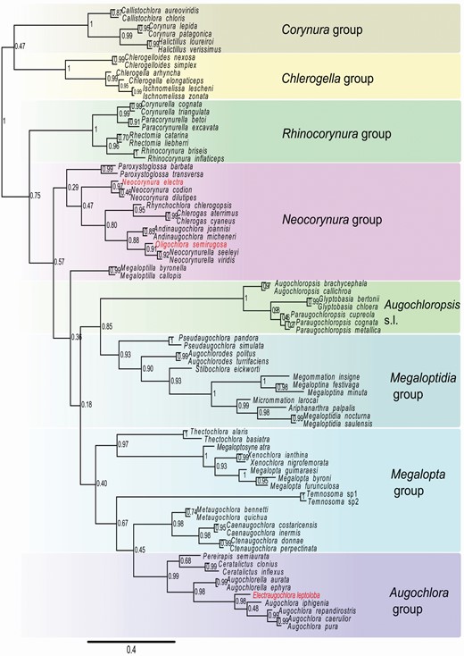
Bayesian consensus tree from morphological data with homoplasy criterion partitioning for Augochlorini bees. Node numbers represent the posterior probabilities. Genus groups coloured as in Figure 2. Red font indicates fossil species.
The model DIVALIKE yielded the highest likelihood and best AICc scores for ancestral range estimation for the Augochlorini phylogeny [see Supporting Information (Table S5) for statistics]. Those values were similar to DEC, and the ancestral range estimations were similar between all methods, with the same range reconstruction for most nodes. The most recent common ancestor (MRCA) of Augochlorini occurred in a composite area including Andean, Atlantic and Pacific endemism areas (Fig. 3). A first vicariant event split ancestors of the Corynura group in the Andean area and the remaining Augochlorini in the Atlantic + Pacific area. A second event split the ancestor of the Chlerogella group from the Pacific and the remaining Augochlorini in the Atlantic area. The most different scenario came from the BAYAREALIKE analysis, where both events were reconstructed as dispersions. All reconstructions indicated that the Atlantic endemism area was the ancestor range for all Augochlorini genus groups between 55 to 40 Mya. Pacific endemism areas were occupied twice around 35 Mya with further dispersions to the Atlantic and Amazonian areas. The Amazon endemism area was occupied several times with occupation until 10 Mya. The occupancy of the Antillean endemism area is attributed to multiple dispersal events and the Nearctic endemism area was occupied at least three times from 15 to 10 Mya.
DISCUSSION
Partitioning and total-evidence analysis
Total-evidence analyses have been widely used in different groups of organisms to contemplate the largest phylogenetic information available (Nylander et al., 2004; Ronquist et al., 2012a; Pyron, 2017). In our study, we used the concept of total evidence in its broadest sense, using four genes and discrete characters from internal and external morphology as a source of phylogenetic information, in addition to including fossil taxa as terminals. We estimated the phylogenetic relationships of fossil lineages of Augochlorini (never tested phylogenetically before) and calculated the divergence time of more than 30 terminals from which molecular sequences are not available.
In the past decades many researchers have studied the evolutionary history of different groups of bees (such as Almeida et al., 2012; Cardinal & Danforth, 2013; Martins et al., 2014; Martins & Melo, 2015; Gonçalves, 2016; Cardinal et al., 2018; Martins et al., 2018; Almeida et al., 2019; Aguiar et al., 2020). Most of these works were conducted with molecular data, resulting in phylogenies dated by node-dating under Yule models only with extant lineages. Recently, Gonzalez et al. (2019) conducted a work with a total-evidence approach including fossils and phylogenies dated by tip-dating under FBD models. However, in this present study, we take it a step further in reconstructing the phylogeny and biogeography history of Augochlorini. In addition to conducting total-evidence analysis using tip and node-dating under the FBD model, we also included internal morphology data and re-evaluated the partitioning of the morphological data according to the homoplasy criterion (Rosa et al., 2019).
In general, our study is pioneering in using partitioning of morphological data in a total-evidence approach. The use of data partitioning considerably increased the MgL in both models with independent data (i.e. only with morphological or only molecular data) and in models with combined data. This result was already expected since data partitioning is an efficient way to accommodate the among-character rate variation in complex data sets (Nylander et al., 2004; Kainer & Lanfear, 2015; Rosa et al., 2019).
Two partitioning strategies must be taken into account as they have presented consistent results. In the partitioning of morphological data, our results showed that the inclusion of non-informative characters in the no-homoplasy partition significantly increased the MgL (KRS > 5). In the partitioning of molecular data, our results showed that the inclusion of exons and introns in their own partitions (Model B) dramatically increases the MgL compared to simple gene-by-gene partitioning (Model A). Both strategies played significant roles in the combined analyses and should be encouraged in total-evidence approaches in Bayesian inference.
Systematics of Augochlorini
The expanded morphological data, inclusion of more extant and fossil species, and more advanced analytical methods provided a more robust hypothesis of augochlorine generic relationships compared to that of Gonçalves (2016). The genus groups are more stable under the new analysis and we are favourable to the maintenance of their use. The monophyly of the Neocorynura and the Megalopta groups was not consistently recovered among multiple as in the preferred total-evidence analysis (Fig. 2).
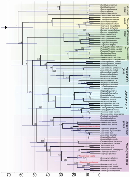
Total-evidence time-calibrated consensus tree for Augochlorini bees. Bars represent the 95% Highest Posterior Density interval for node ages, node numbers represent the posterior probabilities. Genus groups coloured as in Figure 1. Absolute time scale presented in millions of years. Red font indicates fossil species.
A significant advance is related to the position of Augochloropsis s.l., which was uncertain in previous analyses (Engel, 2000; Gonçalves, 2016). Here all analyses recovered this clade as related to the Megaloptidia group and the Augochloropsis lineage could be included in this informal group for simplicity. Augochloropsis s.l. is the largest genus of the tribe (Moure, 2012) and division into three separate genera, Augochloropsis, Glyptobasia Moure, 1941 and Paraugochloropsis Schrottky, 1906 is advocated here. Relationships between these three lineages were studied by Santos (2014) and Celis & Cure (2017) with morphological data. Despite a few inconsistencies between these studies, both hypotheses indicatedthe monophyly of the three taxa. Unfortunately, the large number of valid and available species names and the uncertainty of several species identities makes it difficult to adopt this classification before taxonomic revision.
A few modifications at genus level are necessary to make the classification of the tribe entirely based on monophyletic lineages. Megalopta atra Engel, 2006 has a distinctive morphology that is significantly discrepant from other Megalopta species, and previous studies already called attention to its close relationship with Xenochlora Engel, Brooks & Yanega, 1997 (Tierney et al., 2012; Gonçalves, 2016). Recently, Engel (2020) provided a new subgenus for this species, MegaloptosyneEngel, 2020, which is here recognized at the genus level to avoid the paraphyly of Megalopta. Alternative resolutions are not adequate, the transference of this species to Xenochlora is not supported by the morphological analysis, and the synonym of Xenochlora under Megalopta seems to be retrograde.
Secondly, Chlerogella is not monophyletic in our analyses. IschnomelissaEngel, 1997 was considered as a subgenus of Chlerogella by Michener (2007), but Moure (2012) and other authors maintain both genera. This clade has 43 species with different degrees of elongation of malar space and the proposal of a new genus for Chlerogella arrhyncha, Engel, 2010 and allied species depends on a broader phylogenetic analysis including more species. The best evidence to date suggests synonymizing both genera.
Relevance of internal morphology
The internal characters have been used in bee systematics since Michener (1944) with subsequent efforts by many authors (e.g. Roig-Alsina & Michener, 1993; Alexander & Michener, 1995; Packer, 2003). This data source gained fresh attention from researchers (e.g. Porto et al., 2016 a, b; Meira & Gonçalves, 2018) as part of a global renaissance of phenomics (Deans et al., 2012). Our analysis of internal morphology provided 24 characters for 48 species, which corresponded to 25% and 42% of total characters and terminal species, respectively. The inclusion of these characters provided a morphology-based topology (Fig. 1) more resolved and robust than external characters alone (see figs S3-S4 of Gonçalves, 2016). Beyond their direct impact in the analysis, those characters provided putative synapomorphies for most internal clades as suggested by the character optimization on the total-evidence tree (Supporting Information, Fig. S1). Some of those findings can be evaluated in parallel with detailed studies carried out with internal morphology of the head (Porto et al., 2016c; Porto & Almeida, 2019), the mesosoma (Porto et al., 2016b) and the sting (Packer, 2003).
In the case of the mesosoma, the relevance of internal characters for augochlorine phylogeny was already explored by Meira & Gonçalves (2018). For example, their analysis provided two synapomorphies from the prosternum and scutellar-axillar complex for the clade (Megaloptidia group, (Neocorynura group, (Augochlora group, Megalopta group))), a lineage not recovered in other studies using only external morphological characters (Danforth & Eickwort, 1997; Engel, 2000, Gonçalves, 2016). This tagma provided most of the internal characters included here (29 character statements).
Internal characters of the head gave an additional synapomorphy for the clade Augochloropsis + Megaloptidia group (147:1; median expansion of epistomal ridge adjacent to the insertion of eutentorial arm to head capsule long, length more than 1.5× antennal foramen diameter) and also for Augochlora + Megalopta group (148:1; ventral ridge of clypeus reduced to a small strip, less than 0.33× antennal foramen diameter). Both characters were modified from Porto et als (2016c) analysis of head internal sclerites of corbiculate bees. The topology (Chlerogella group + others) was recovered for the first time with this data set (Supporting Information, Fig. S1), and the folded apodeme of frontal muscles of the pharyngeal plate (142:1) was the unique synapomorphy. The pharyngeal plate was recently studied in detail by Porto & Almeida (2019) for Apoidea lineages, and the folded apodeme can be seen in their figure 8 for Augochlorella aurata (Smith, 1853). Our results support their opinion that the pharyngeal plate could have information for phylogenetic inference at multiple levels.
The seven characters derived from the sting only gave synapomorphies at the genus level, for example for Augochloropsis s.l. (182:1; 7th hemitergite, lamina spiracularis, apodemal region of the marginal ridge with spine) and Augochlora (186:0, furcula, dorsal arm not expanded). The gradually angled apical process of the second valvifer (184:0) was a synapomorphy for Megalopta and also for Augochlorella plus Augochlora. Packer (2003) presented a comparative description of bee sting apparatus, finding new putative synapomorphies for many family-group taxa. The author also suggested that systematic studies on the above species should include analysis of the sting apparatus, a view corroborated here.
Biogeography
Danforth et al. (2004) suggested that the Augochlorini ancestor dispersed from Africa to South America between 70 to 55 Mya. This view should be examined carefully, because the position of Caenohalictini as a sister group to the remaining Halictini s.l. (Gibbs et al., 2012; this study) offers an alternative hypothesis of a South American origin of Halictinae s.l. The biogeography of the tribe is intrinsically linked to the Neotropical region, particularly with the Atlantic endemism area. The Andean endemism area was colonized once, and the Pacific, Amazonian, Antillean and Nearctic regions were colonized multiple times during the evolution of the tribe (Fig. 3). Despite the antiquity of Augochlorini recovered by the present analysis, most of the genera started diversifying during the Miocene, as found for other endemic insects such as butterflies (Chazot et al., 2018; Brower & Garzón-Orduña, 2020).
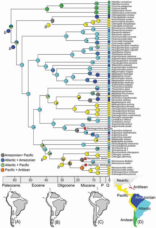
Time-calibrated consensus tree and ancestral range estimation for Augochlorini bees. Pie charts on nodes represent ancestral range estimation under the highest likelihood of DIVALIKE. The nodes with alternative ancestral range reconstructions are indicated by b for BAYAREALIKE analysis. Reconstructions of South America uplands of A, Palaeocene; B, Late Eocene and C, Miocene, based on Lundberg et al. (1998) and Aceñolaza (2000) (uplands in grey); D, endemism areas used herein. Absolute time scale presented in millions of years. P = Pliocene, Q = Quaternary
Most ancestral range reconstructions favoured a vicariant event at the base of the tribe, the Corynura group splitting from the remaining Augochlorini during the Palaeocene-Eocene transition; however, BAYAREALIKE analysis suggested repeated dispersals from the Atlantic endemism area, this latter scenario being favoured by the stable condition of the Brazilian Plateau (Lundberg et al., 1998; Aceñolaza, 2000; Antonelli et al., 2009; Hoorn et al., 2010). A similar pattern was found for Caenohalictini, with the colonization of the Andean region by some species of Caenohalictus and also twice in the Pseudagapostemon clade (Gonçalves & Melo, 2010). The vicariant event can be attributed to Atlantic marine transgression that occurred in this period and is invoked to explain the same pattern found in many other organisms (Luebert et al., 2020); the isolation could also be maintained by Miocene introgressions (Morrone, 2018). The diversification of Corynura group genera occurred after the Miocene and Halictillus loureiroi (Moure, 1941) represents an isolated dispersal event from the Andean to the Atlantic area. Disjunct distributions between Andean and Atlantic plants are known to occur over a long time range from 27 to 1 Mya (Luebert et al., 2020). Despite possible connections of the southern Andes with the central and northern Andes during the Cenozoic (Ramos, 2009), the Corynura group did not disperse to the north (González-Vaquero & Roig-Alsina, 2017).
The second event, around 55 Mya, was the split of the Chlerogella group and the remaining augochlorines in the Amazonian-Pacific and Atlantic areas, respectively. The cause can be the marine transgressions in the Neotropics in the Amazon Basin (e.g. Amorim & Pires, 1996; Nihei & Carvalho, 2007; Morrone, 2014). While many other terrestrial organisms (plants, invertebrates and vertebrates) followed this same pattern, due to the great number of recorded transgressions in this region, similar distributions may be convergent due to vicariance events at different ages (Nihei & Carvalho, 2007). The diversification of the Chlerogella group occurred around 37 Mya with the split of the Chlerogelloides ancestor in the Amazon and Chlerogella s.l. in the Pacific area. At the end of the Eocene, northern South America had three uplands (Antonelli et al., 2009): Central, the northern Andes and the Guiana Shield, and those areas could house the ancestors of the Chlerogella group during the multiple marine transgressions. Some species of Chlerogella are distributed in the Mesoamerican Dominion while others are restricted to the Pacific Dominion. Further analysis is necessary to fully understand the biogeography of the Chlerogella group, with a broader representation of included species.
The remaining lineages of the Augochlorini (Rhinocorynura group (Megaloptidia group, (Neocorynura group, (Augochlora group, Megalopta group)))) were established during the Eocene. The ancestral range of these clades was the Atlantic endemism area according to all reconstructions (Fig. 3). Climate and associate floristic changes may have been an important factor modulating early diversification of Augochlorini, since the basal splits of the tribe were concomitant with the Palaeocene-Eocene Thermal Maximum (56 Mya), when temperatures increased rapidly associated with increased plant diversity and origination rates (Jaramillo et al., 2010). Members from all groups dispersed to the Amazon and Pacific areas, with the Augochlora and Neocorynura groups also colonizing the Antillean endemism area.
The Pacific endemism area was essential to the diversification of the Megalopta and Neocorynura groups in addition to the Chlerogella group. The events of colonization of this endemism area by those groups occurred during the Eocene-Oligocene (Fig. 3) with the diversification beginning in the Miocene, probably triggered in response to the late orogeny of the Andean mountain range (Ramos, 2009; Jaramillo et al., 2017). A similar synchronic pattern was detailed by Santos et al. (2019) for poison dart frogs and Almeida et al. (2019) for Neopasiphaeini bees. The ancestor range reconstruction for the Neocorynura group should be analysed carefully since the first nodes present low support (Fig. 2). AndinaugochloraEickwort, 1969, Chlerogas Vachal, 1904, NeocorynurellaEngel, 1997 and Rhynchochlora Engel, 2007 are associated with the Pacific Dominion, while Neocorynura has a broad distribution in the Neotropical region. More interesting is the distribution of Megaloptilla Hurd & Moure, 1987, with one species recorded for the Pacific Dominion and another for the Mesoamerican Dominion. In the Megalopta group, the Caenaugochlora s.l. lineage is restricted to Pacific endemism area (both Dominions), while the lineage of Megalopta s.l. has a widespread distribution in the Neotropical region, except for the Caribbean. The lineages near the base of both groups are mostly restricted to the Atlantic area, Paroxystoglossa Moure, 1940 in the case of the Neocorynura group and Thectochlora in the case of the Megalopta group.
A critical point in the biogeography of Augochlorini is the Antillean endemism area. This subregion was also colonized by the Neocorynura group, but only fossils are known. The most recent ancestor of (Neocorynura (Neocorynurella + Andinaugochlora)) dates from 35 Mya, concomitant to the GAARlandia land bridge, a connection between South America and Central America that allowed interchanges by several groups (Iturralde-Vinent, 2006; Toussaint et al., 2019; Roncal et al., 2020). In the Augochlora group, Electraugochlora leptoloba also could be related to some past connections of Central America. The only extant Augochlorini in the Caribbean islands are a few species of Augochlora, Pereirapis and Temnosoma, and their occurrence could be considered as consequences of more recent events given the relatively young ages recovered overall for intrageneric diversification.
As predicted by Michener (1979) the halictines are not diverse in the Amazon (Gonçalves & Melo, 2010). The Amazonian area was occupied several times by all augochlorine lineages, except for the Corynura group, and these occupations occurred in the Late Miocene as dispersal events from Atlantic and Pacific areas (Fig. 3). The whole scenario is different from the Tapinotaspidini, in which a clade originated in the Amazon Basin about 30 Mya (Aguiar et al., 2020) and was confined in the Guiana Shield during the most critical phases of marine transgressions. According to several authors (Lundberg et al., 1998; Aceñolaza, 2000; Ortiz-Jareguizar & Cladera, 2006; Antonelli et al., 2009; Hoorn et al., 2010; Jaramillo et al., 2017), Amazonian lowlands were affected by rising of the sea level during the Cenozoic with the greater influence from the Pebas System in the Miocene. The diversification rates of terrestrial fauna and flora decreased during the Miocene to recover before the Pebas System (Hoorn et al., 2010; Chazot et al., 2018 and references therein) with the uplift of the northern Andes and a drop in sea level 10 Mya (Hoorn et al. 2010). The augochlorine lineages inhabiting uplands in the Brazilian Shield and the Andes diversified in Amazonia after those events 10 to 7 Mya. Xenochlora meridionalisMelo, Faria & Santos, 2019 was recently described from the Atlantic endemism area, indicating recent dispersals from Amazonian to Atlantic endemism areas (Melo et al., 2019).
CONCLUSION
We provide a revised phylogeny for Augochlorini with the inclusion of a detailed morphological data set including internal skeleton characters and five fossil species as tip-dating points along with molecular data. The homoplasy-based partitioning of morphological data to reconstruct age estimates under a total-evidence framework is pioneering and yielded robust results for the group. The homoplasy criterion applied to the morphological data combined with the molecular ad hoc partitioning resulted in a significant increase in the MgL, and is therefore highly recommended for use in tip-dating analyses. We confirm that Augochlorini diversification started in the Palaeocene with the establishment of most genus groups during the Eocene. Based on ancestor range estimation, we proposed a biogeographic scenario for the early diversification of the tribe, revealing the importance of the Brazilian Plateau for most lineages. Multiple dispersals to Amazonia, Central America and North America with some returns to the Atlantic endemism area were also recovered.
SUPPORTING INFORMATION
Additional Supporting Information may be found in the online version of this article at the publisher’s web-site:
Table S1. GenBank accession numbers of exemplars and origin of samples used in this study.
Table S2. Morphological character matrix.
Table S3. Descriptions of morphological characters and character states.
Table S4. Endemism areas and references for distribution.
Table S5. Ancestor range estimation statistics.
Figure S1. Optimization of morphological characters in the total-evidence tree.
Figure S2. Comparative morphology of internal structures and mandibles of Augochlorini: (A) mandible internal view, Temnosoma; (B) mandible outer view, Thectochlora alaris; (C) mandible outer view, Paracorynurella excavata; (D) mandible inner view, Glyptochlora bertonii; (E) mandible inner view, Augochlora amphitrite; (F) tentorium and hypostoma lateral view, Ariphanarthra palpalis; (G) hypostoma and second tentorial bridge of Augochlora iphigenia; (H) hypostoma and second tentorial bridge ventral view, Habralictus canaliculatus; (I) 7th hemitergite dorsal view, Augochloropsis callichroa; (J) 7th hemitergite dorsal view, Dialictus sp; (K) 7th hemitergite dorsal view, Peudagapostemon pissisi; (L) 8th hemitergite dorsal view, Augochloropsis callichroa; (M) furcula anterior view, Megalopta guimaresi; (N) prosternum ventral view, Ariphanarthra palpalis; (O) prosternum anterior view, Ariphanarthra palpalis; (P) prosternum lateral view, Ceratalictus clonius.
Figure S3. Homoplasy-partitioned morphology tree for Augochlorini bees, original tree with outgroups.
Figure S4. Total-evidence time-calibrated tree for Augochlorini bees, original tree with outgroups.
ACKNOWLEDGEMENTS
We are grateful to Gabriel Melo for sharing unpublished data and his ideas on data partitioning and for helpful comments on the monograph of O.M.M. We also thank Anderson Lepeco for suggestions on the final version of this manuscript, and two anonymous reviewers and the associate editor for critical evaluation.
R.B.G. conceived the study, re-analysed the codification of the morphological characters and dealt with molecular data selection alignment. R.B.G. also carried out the ancestor range estimation analysis, wrote the first version of the manuscript and is responsible for the taxonomic treatments. O.M.M. studied and codified the internal characters and carried out all dissections and illustrations. B.B.R. conducted all phylogenetic analyses and refined the new method to combine homoplasy-partitioned morphology with DNA in the total-evidence framework. All authors contributed to the final version of the manuscript.
DATA AVAILABILITY
The data underlying this article are available in GenBank Nucleotide Database at https://www.ncbi.nlm.nih.gov/genbank/, and can be accessed with accession numbers given in Table S1.
REFERENCES
