


Different approaches have been used to estimate the economic benefits of reducing undernutrition and to estimate the costs of investing in such programs on a global scale. While many of these studies are ultimately based on evidence from well-designed efficacy trials, all require a number of assumptions to project the impact of such trials to larger populations and to translate the value of the expected improvement in nutritional status into economic terms. This paper provides a short critique of some approaches to estimating the benefits of investments in child nutrition and then presents an alternative set of estimates based on different core data. These new estimates reinforce the basic conclusions of the existing literature: the economic value of reducing undernutrition in undernourished populations is likely to be substantial.
Introduction
In September 2015, the UN General Assembly adopted a set of Sustainable Development Goals (SDGs) as successors to the Millennium Development Goals (MDGs) that ran from 2000 to 2015. The scope of these goals is wide; there are 17 SDGs compared to the eight MDGs. The increase in the number of targets being monitored is even greater. There are 169 targets in the SDGs while the MDGs had only 18. Reduction of all forms of malnutrition is a target under the second goal of ending hunger. One step to achieve this would be to reduce the rate of stunting by 40 percent. As there were 161 million stunted children under five in 2015 (International Food Policy Research Institute 2015), this is a major challenge. To address this, finance ministers and other policy makers have to assess the benefits and costs against meeting other goals, including the 168 other SDG targets.
One input in the assessment of which investments to prioritize is estimates of the economic benefits of reducing undernutrition, as well as estimates of the costs of investing in such programs. In addition to the economic use of such information, these estimates often are employed for advocacy, frequently on a global scale. Various approaches have been used to provide such assessments of the economic benefits of improved nutrition and to package these as regional or global estimates. While many of these studies are based ultimately on evidence from well-designed efficacy trials, all require a number of assumptions to project the impact of such trials to larger populations and to translate the value of the expected improvement in nutritional status into economic terms.
The argument that some interventions for improving nutrition are investments on par with other productivity-enhancing expenditures rather than simply a form of governmental social spending designed to improve welfare and equity is hardly new (Berg and Muscat 1972). However, contemporary and often novel data are being brought to bear to address some of the inherent challenges to quantifying the returns to investing in children. Among these challenges is the difficulty in linking changes in stunting or anemia in young children to enhancements in their productivity over their lifetime, as well as to assign a value to averted mortality in a metric that permits direct comparisons with other impacts and with costs. While various randomized trials can assess the impact of a nutrition intervention on the health of a target population over relatively short segments of the lifecycle, with the exception of a few notable longitudinal studies (Hoddinott et al. 2013a), additional data or parameters derived from outside of the treatment population are required to estimate the economic value of the improvements in nutrition in terms of changes in productivity. For example, the improvements in under-five stunting from a specific project or from a meta-analysis of similar programs can be applied to parameters that estimate the relationship of stunting to grades of schooling attainment and then to earnings using the global body of evidence from Mincerian and similar returns to schooling. In contrast, the few longitudinal studies that track an improvement in nutrition to the beneficiaries’ adult lives have the advantage of avoiding constructing such a synthetic chain, but at a potential sacrifice in external validity that stems from extrapolation outside the relatively small and selected communities in which the currently available longitudinal studies over decades were conducted and from the necessity of assuming that an intervention conducted two or more decades previously would have the same impact if conducted today.
This paper provides a short critique of various approaches to estimating the benefits of investments in child nutrition and then presents an alternative set of estimates. While this new calculation of benefits is not free of strong assumptions, going from initial estimates of improvement in height to aggregated regional but global gains, and as the core data differ from others in the literature, they reinforce the basic conclusions of the existing literature. Despite the differences in methodology between the various estimates in the literature of the economic value of reducing undernutrition, to a fair degree the collective body triangulates the investment potential in nutrition.
A Brief Critique of Approaches to Economic Analysis of Nutrition Programs and Their Impacts
The various approaches to estimating the benefits of improved nutrition—or, alternatively, the foregone gains or opportunity costs of undernutrition—draw upon a common body of experimental and programmatic evidence accumulated by health professionals and often summarized using meta-analyses and systematic reviews. A recent review was provided by Bhutta et al. (2013), in which the authors modeled the impact of increasing the coverage of 10 evidence-based nutrition programs to 90 percent of the population of 34 countries with the highest burden of undernutrition. They estimate that this scaling-up would reduce child mortality by 15 percent and stunting by 20 percent. Approaches to calculating the economic benefits from this and similar program impacts share the requirement of discounting future benefits, although the discount rates employed vary; many studies acknowledge the absence of consensus on discount rates and present results using a range of such discount rates. This section reviews salient features of different approaches to the common objective.
Project Benefit-Cost Analysis
While many studies of the value of improved nutrition report the net present value of potential investment—that is, the discounted stream of benefits—often the discounted benefits are reported as a ratio relative to costs. This standard approach to estimating the total benefits and costs of a project provides a clear economic interpretation and a guideline for investment when benefits exceed costs. While often based on outcomes and costing data obtained from investment at scale, the data nevertheless do not have global coverage. Stylized benefits and costs based on a wider literature, however, have been applied to derive global patterns in returns to nutrition interventions (Behrman, Alderman, and Hoddinott 2004; Horton, Alderman, and Rivera 2009; Horton and Ross 2003). As benefit-cost ratios from one sector of investment can be compared to ratios from very different types of investments, this approach allows comparisons across diverse sectors. Individual nutrition programs have been shown to have as high or higher rates of return than those in traditional-development investments such as those in physical infrastructure in such comparisons (Lomborg 2004).1
However, benefit-cost ratios by themselves do not tell if the total gains are likely to be very large or relatively small. Two projects may have identical benefit-cost ratios but very different potential gains from implementation because they have very different benefits and costs even though the benefit-cost ratios are the same (e.g., project A with benefits of $3,000 and costs of $1,000 per affected person and project B with benefits of $3 and costs of $1 per affected person both have benefit-cost ratios of 3) or because they can be scaled up to very different-sized populations. Therefore, it may be advantageous to consider the total benefits and costs in addition to the benefit-cost ratios of alternative projects.
To calculate benefit-cost ratios, it is necessary to place the value of all impacts and all costs into the same metric, which in some cases is very difficult. For example, consider the case in which there are two impacts—increasing productivity and averting mortality—and costs are measured in monetary terms. Measuring increased productivity also in monetary terms may be relatively straightforward, but placing reduced child mortality in the same metric as increased productivity requires strong assumptions.2 Alternatively, benefit-cost ratios in this case can be calculated in terms of productivity gains alone, with the recognition that the unknown value of reduced mortality is surely positive and, thus, the estimated benefit-cost ratios that exclude this category of benefits are lower bounds. If the benefit of a lower bound exceeds the investment criteria, then the full benefits will as well.
One issue with this approach—as well as all other attempts to provide regional or global estimates of either benefits or costs—is that these estimates often cover a scale beyond that of the programs from which the data are derived. It is unlikely that either benefits or costs are constant as the coverage increases. This reflects issues such as staffing constraints and potential dilution of service quality, as well as the difficulty of reaching remote areas and of ensuring program participation in subpopulations. Moreover, seldom do estimates consider market-wide and general equilibrium effects of, for example, broadly increasing schooling and labor market participation. Generally, such effects are thought to reduce the benefits through shifting labor supplies outward and lowering wages; however, they might work in the opposite direction if, say, more-schooled populations increase demands relatively for goods and services that utilize more-schooled inputs.
Estimates of Aggregate GNP Loss Due to Nutritional Status of Current Population
A set of studies report estimates of additional labor force productivity based on either the current stunting rates of the labor force (Martinez and Fernández 2008, 2009) or the average height or predicted average heights of the population (Horton and Steckel 2013). Both stunting rates and average heights are readily available from surveys and can be translated into productivity loss using best-practice estimates of impact of nutrition on schooling and earnings. For example, Horton and Steckel (2013) use data from a range of microstudies on the relationship of wages and nutrition, along with estimates of the average height in various countries to model the loss of potential income over the twentieth century from undernutrition, as well as provide a projected path of gains in the twenty-first century as nutrition improves. They determine that undernutrition cost the world 8 percent of GNP in the twentieth century and that this will decline to 6 percent in the first half of the current century. They indicate the assumptions that might increase or decrease the general results. For example, the results do not include the impact of iron or other micronutrients. Because there is a documented relationship between iron and cognition and only a partial correlation with height, this assumption may contribute to an underestimation. Conversely, if the share of wages in GNP is less than the assumed 50 percent, the reported loss may be higher than actual.
The studies by Martinez and Fernández (2008, 2009), jointly conducted for the Economic Commission for Latin America and the Caribbean (ECLAC) and the World Food Program, also include the mortality and morbidity of young children, along with estimates of the lost productivity of the underweight members of the current work force in the baseline year. The 2008 report estimated that undernutrition—in particular, low birth weight and underweight—resulted in a loss of between 1.9 and 11.4 percent of GNP for countries in the Caribbean and Central America, with the lowest loss in Costa Rica and the highest in Guatemala. Over 90 percent of this was attributed to lost productivity, split equally between less schooling and the lost wages of children who died before entering the workforce. The former component of lost productivity included grade repetition as well as dropout associated with undernutrition, albeit not with longitudinal studies. The latter estimate uses a common approach to costing early mortality based on expected lifetime earnings, but one that usually calculates benefits without subtracting either the resources that would have been required for educating the individual or the value of consumption for that individual. Health expenditures accounted for only 6.5 percent of the total. While the ECLAC studies compared the losses due to malnutrition to the current budget for health services, this served only as a benchmark; the methodology was not designed to explore a direct path between specific investments and outcomes. The African Union Commission also employed the retrospective methodology used by ECLAC. In their initial set of studies, the African Union found that Egypt lost 1.9 percent of GNP due to undernutrition, while Uganda lost 5.6 percent and Ethiopia lost 16.5 percent. A subsequent study claimed a loss of 10.3 percent of GNP due to undernutrition in Malawi (African Union Commission 2015).
Estimates of GNP Loss Due to Neglecting Undernutrition in a Cohort of Children
The ECLAC studies also provided projections of the loss due to undernutrition for the current cohort of children under five years of age. As there are fewer individuals than those in the entire current work force and as these children will not enter the labor force for years and, thus, any estimates of lost productivity require discounting, these losses are much lower than those mentioned above. The loss due to undernutrition in this set of estimates ranges from 0.5 percent of GDP for Guatemala to virtually nothing for Costa Rica.
Similarly, a recent study from Fink et al. (2016) estimates the impact of inaction with regard to reducing undernutrition on schooling. This results in substantial economic costs, calculated at $176.8 billion per cohort year at nominal exchange rates and $616.5 billion at purchasing power parity–adjusted exchange rates.
Aggregate Budgetary Cost of Scaling-Up Nutrition
A few detailed studies (Horton et al. 2010; Bhutta et al. 2013) have taken a more conventional look at costs, in terms of the budget needed to finance a proven set of interventions rather than the opportunity costs or losses that malnutrition represents, as in the ECLAC studies. These studies calculate the costs of expanded coverage of a set of best-practice programs. Both Horton et al. and Bhutta et al. estimate outcomes in terms of age-specific mortality and nutritional status with confidence intervals provided—a feature that is not always offered in similar studies. However, they do not attempt to place these outcomes in terms of productivity or savings in health care.
The projections by Bhutta et al. (2013) differed slightly from Horton et al. (2010), but not at a substantive level. The earlier study estimated the total costs of scaling-up programs at $11.8 billion per year, a sum that included an estimated $1.2 billion for building capacity, as well as monitoring and assessment that is not included in the $9.6 billion per year estimated by Bhutta et al. (2013). The two studies also differ somewhat in the baseline coverage from which program expansion is assumed to occur, as well as in some of the interventions included; Horton et al. (2013) included deworming and therapeutic zinc for diarrhea, which are not covered by Bhutta et al. Conversely, calcium supplements and balanced energy protein supplements in pregnancy are components in only the estimates of Bhutta et al. (2013).
The costs, however, are for scaling-up per se; programs for which coverage already is at a high level (such as vitamin A supplementation) contribute little to the scaling-up budget. Thus, the costs reported are less than the total resources required for providing basic nutritional services, although the methodology can easily be applied to include the costs of coverage at current rates. These costs are not necessarily all public expenses; while the programs reviewed are often run by governments, there are various means through which some costs are recovered from beneficiaries through fees or, in the case of fortification, in the final product price.
As with other estimates of the benefits or costs of scaling-up programs to larger populations, it is necessary to make assumptions on the degree that costs increase as programs expand. To this end, Horton et al. (2010) assumed that the cost per beneficiary for increasing program delivery beyond 80 percent of the population was twice as much as the average cost for reaching 80 percent of the population. However, there is relatively little available evidence from which to verify or refute this assumption. Similarly, there is relatively little evidence as to whether the expected benefits from reaching hard-to-cover populations rise faster than the costs due to their relative deprivation or whether the benefits decline due to dilution of service quality as capacity constraints begin to bite.3
Combining Productivity Gains and Budgetary Costs for Benefit-Cost Estimates
Hoddinott et al. (2013b) ask what would be the economic benefit if the 10 programs modeled in Bhutta et al. (2013) achieved a 20 percent reduction in stunting in various countries. They estimate the increase in productivity that this improvement will produce by converting the change in stunting to a change in per capita consumption using results from a longitudinal study of the impact of moving a two-year-old child from being stunted to not being stunted in Guatemala (Hoddinott et al. 2013b). Then, to be conservative, they scale this estimate down by 10 percent. Both the assumed proportional reduction in stunting and the proportional increase in earnings are common to all regions studied in this paper; differences in estimated benefits across countries stem from the differences in the projected growths in income per capita. Results are particularly sensitive to the latter. The populations studied are cohorts of children under two years, and their productivity gains are estimated in terms of a proportion of the incomes per capita that are expected when they enter the labor force; therefore, the larger the income per capita, the greater the economic returns. While the high-burden countries studied in their paper are currently relatively low-income economies, some have impressive recent growth rates. These predicted gains were compared to the cost for the full package of interventions from Horton et al. (2010), which vary across countries, resulting in benefit-cost ratios ranging from 3.8 for the Democratic Republic of the Congo to 34.1 for India. As illustrated in this paper, such results vary according to assumed income growth rates, as well as, of course, discount rates; further, according to assumed years in the labor force (Horton and Hoddinott 2015) but under all assumptions, the benefit-cost ratios compare favorably with other investments such as schooling.
An Alternative Approach to Estimating the Economic Value of Improved Nutrition
As an alternative approach for this paper, we estimate the economic benefits of improvements in stunting if the trends reported by UNICEF (see table 1, adapted from UNICEF, WHO, and World Bank 2014) continue relative to a no-improvement counterfactual. We also look at an accelerated case that assumes that the World Health Assembly (WHA) target of 40 percent reduction in stunting is adopted as an SDG and achieved in all regions by 2030; that is, the target is assumed to be reached at a slightly slower rate than would be necessary to achieve the WHA target by 2025.
Under 5 Population, Malnutrition Rates and Projections by Region
| Regions | Under 5 population (2015) | Stunting rate (2015) (%) | Stunting rate (2020a) (%) | Stunting rate (2025a) (%) | Stunting rate (2030a) (%) |
|---|---|---|---|---|---|
| South Asia | 168,384,399 | 35.60 | 30.94 | 26.85 | 22.75 |
| East Asia and Pacific | 152,064,093 | 10.18 | 7.28 | 5.46 | 3.63 |
| Latin America and Caribbean | 53,550,493 | 10.18 | 8.58 | 7.32 | 6.05 |
| Middle East and North Africa | 49,854,118 | 16.81 | 14.70 | 12.92 | 11.13 |
| Eastern Europe and Central Asia | 28,814,898 | 9.47 | 7.45 | 6.00 | 4.55 |
| Africab | 160,159,062 | 35.81 | 33.40 | 31.15 | 28.90 |
Notes: All data in the table are adapted from (UNICEF, WHO, and World Bank Group 2014).
aProjected rates according to trend.
bAfrica regional estimates are calculated using data from the Eastern and Southern Africa and West and Central Africa Regions.
The approach used to map these improvements in stunting bears a resemblance to that reported in Horton and Steckel (2013) in that we assume benefits from improved nutrition are distributed throughout the population. This differs from changes in stunting that focus on populations that have height-for-age Z scores (HAZ) just below -2, which is the cutoff that is commonly used to indicate stunting rates. In order to determine the improvements in the nutritional status of the general population associated with improvements in stunting rates, we use a direct mapping between changes in stunting at a given starting point and the change in average HAZ score based on the normally distributed WHO reference data for stunting (see Annex table 1). We concentrate on productivity impacts; as noted in the ECLAC studies as well as Alderman and Behrman (2006), while there are savings in health expenditures associated with improved nutrition, these are comparatively small relative to expected improvements in productivity.
For a given predicted change in HAZ for young children such as those in the data found in the UNICEF projections, we can estimate the expected change in grades of schooling attainment that will be completed by a cohort using a coefficient of a 0.678 increase in grades of completed schooling for a 1.0 change in HAZ estimated in a longitudinal study in Zimbabwe (Alderman, Hoddinott, and Kinsey 2006). This step, then, resembles the mapping of changes in consumption predicted given changes in stunting and a coefficient from a longitudinal study from Guatemala in Hoddinott et al. (2013a).
There is much literature on the expected increase of earnings that results from increased schooling. Orazem, Glewwe, and Patrinos (2009) use 63 data sets from 42 developing countries to bracket the expected return to an additional grade of schooling attainment between 7.5 percent (rural) and 8.3 percent (urban). We employ the rural estimate and assume that the labor share of Gross National Income (GNI) is 50 percent, in common with Horton and Steckel (2013).4 We apply this to the estimated GNI per capita in a given year using regional growth rates from the World Bank (2015). Those projected growth rates, however, only extend to 2017. In order to extrapolate beyond 2017, we assume that the growth rate declines by 1 percentage point in each region after 2017. As we have no empirical basis for any long-term trend of GNI, the reduction beyond 2017 can be viewed as an ambiguity risk premium.
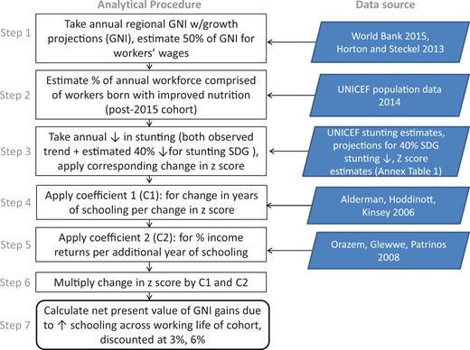
Analytical flow chart of the core model
The gains, of course, require additional investments. Thus, we also estimate the cost of achieving the improvements in stunting with a modification of Hoddinott et al. (2013b). In particular, we take the annual costs from Horton et al. (2010) for different interventions and estimate the cost of nine of the 10 evidence-based nutrition interventions that form the basis for the benefit-cost calculations in Hoddinott et al. (2013).5 These are summed over the life of a child from conception and thus include the cost of maternal supplementation, as well as iodine fortification for the mother. Community-based nutrition is included for two years from birth while complementary feeding is included from six to 24 months. Vitamin A supplementation begins at six months and continues to 60 months while deworming begins at 12 months and also continues to 60 months. Both complementary feeding and community treatment of acute malnutrition are provided to a subset of the population as assumed in Hoddinott et al. (2013b), 80 percent for the former and far less for the latter.6
The scenarios of benefits are for the marginal improvement over baseline under two assumptions. The benefit-cost ratio is first estimated in terms of marginal costs for making these improvements conservatively, assuming each beneficiary receives no services in the absence of the scenarios studied. While this is unlikely, it is a conservative assumption because it increases the cost and thus reduces the benefit-cost estimate. As the scaling-up of the package of nutrition investments is expected to reduce stunting by only 20 percent, we thus take marginal costs for reduced stunting as the full cost of this package for five times the reduction in the number of stunted children. This cost per package is summed over all children in the scenarios using both 3 and 6 percent discount rates. We illustrate this for the South Asia Region.
How Does This Alternative Approach Compare with Other Approaches?
The results of the estimates of global and regional benefits from reduced stunting are reported in table 2. Using current trends from table 1 and comparing these with no improvement in the base case, stunting in South Asia declines by 8.8 percentage points from 2015 levels by 2025 and 12.8 percentage points by 2030 (36 percent of the initial rates). Among the regions, this is the largest projected decline of stunting in terms of percentage points but not as a percent of initial levels. This improvement results in a total increase in productivity reported in table 2, summed over a generation of $1,497 billion using an annual discount rate of 3 percent. This is more than one-half the GNI of the region in 2015 ($2,742 billion). The magnitude of the estimate is surprising and needs to be parsed. As calculated, in 2035, children from 2015 begin to enter the labor force. Thus, only 2.5 percent of the working age population includes beneficiaries of improved nutrition in that year. Their average height-for-age during childhood increased by 0.14 HAZ due to investments in nutrition, leading to a $0.76 billion increase in the GNI under the assumptions outlined above. The net present value (NPV) of the gains in this year at a 3 percent discount rate would be $0.41 billion, or only 0.015 percent of the initial economy. Ten years later, slightly more than a quarter of the working-age population will have benefited from improved nutrition and the economy will have grown as well. Thus, the NPV of the gain in GNI in 2045 at a 3 percent discount rate for that year alone would be $12.7 billion. In that year, the 2015 cohort retires, with 40 percent of the working-age population benefiting from the upward trend in stature; with the economy growing at a rate faster than the discount rate, the NPV of the value of improved nutrition in that year alone is 1.9 percent of the GNI in 2015. If the target of 40 percent stunting reduction were to be reached by 2030, the NPV of the gains in South Asia for this cohort of workers over their working life would be $2,148 billion at a 3 percent discount rate. This would lead to a $651 billion NPV increase, or a 43 percent increase over the current trend.
Benefits from Reduced Stunting (in Billions of Dollars) Based on Returns to Increased Schooling
| Region | Initial stunting rate (2015) (%) | Base case benefits | Accelerated reduction benefits | ||
|---|---|---|---|---|---|
| 3% discount (% 2015 GNI) | 6% discount (% 2015 GNI) | 3% discount (% 2015 GNI) | 6% discount (% 2015 GNI) | ||
| South Asia | 35.6 | 1,497 (55) | 344 (13) | 2,148 (78) | 497 (18) |
| Sub-Saharan Africa | 35.8 | 234 (14) | 56 (3) | 588 (34) | 144 (8) |
| East Asia and Pacific | 10.2 | 4,498 (36) | 1,033 (8) | 4,498 (36) | 1,033 (8) |
| Middle East North Africa | 16.8 | 98 (8) | 25 (2) | 102 (8) | 27 (2) |
| Latin America and Caribbean | 10.2 | 271 (5) | 72 (1) | 271 (5) | 72 (1) |
| Eastern Europe & Central Asia | 9.5 | 202 (10) | 52 (3) | 202 (9) | 52 (3) |
Notes: Values are in billions of 2015 USD.
Numbers in parentheses are percent of 2015 GNI.
Accelerated benefits are those necessary to reach 40 percent reduction by 2030 or current trend, whichever is the greater improvement.
The second largest reduction in stunting reported in table 1 is from Sub-Saharan Africa, where stunting declines by 6.9 percentage points (17 percent of the initial rate) in 2030 under current trends. This would result in an NPV of benefits in the region of $234 billion using a 3 percent discount rate. The NPV would increase to $588 billion if the target of 40 percent reduction could be reached. Thus, given the relative low current trend in improvement, reaching the target by 2030 would more than double the economic value. However, because East Asia and Latin America, as well as Eastern Europe and Central Asia (CEE/CIS), are already projected to reach 40 percent reduction in stunting by 2030, there is no difference between the base case and the accelerated scenario. Similarly, reaching this target would only make a small difference in the Middle East and North Africa.
East Asia has the largest economy in the study, as well as the fastest proportional reduction in stunting. Thus, the benefits from improving nutrition in that region dominate the totals. Still, the gains in South Asia are by far the largest in terms of the share of its GNI in 2015. In Africa, the NPV is 14 percent of baseline GNI in the slower scenario and is one-third of baseline GNI if improvements are faster. The proportional benefits in terms of GNI are lower in those regions where initial stunting is relatively low. Also, as expected, because the benefits from reducing stunting accumulate in the future when the children enter the labor market, the NPV of the gains are lower with the higher discount rate.
How do these benefits compare to costs? The benefit-cost ratio for South Asia is 81:1, assuming that the investments are applied at the margin and with a discount rate of 3 percent. This is the base case reported in table 3; it used an estimate of cost that is five times the cost of the package of interventions for the children for whom stunting is prevented under the assumption that the package prevents stunting in 20 percent of program recipients (Bhutta et al. 2013). This benefit-cost ratio compares to the estimates of 76:1 and 35:1 for India and Bangladesh at that discount rate using the parameters from Guatemala employed by Hoddinott et al. (2013b). However, part of the difference between the current estimates and the earlier ones reflects assumptions on the duration of labor force participation. Hoddinott et al. (2013b) assume that individuals are in the labor force from age 21 until age 36. If it is assumed that they work until age 50, the benefit-cost ratio for India rises to 134 at 3 percent discount and rises further to 157:1 if the individuals work until age 60 (Horton and Hoddinott 2015).
Alternative Estimates of Benefit-Cost Ratios from Reduced Stunting for South Asia
| Scenario & key assumptions | Discount rate (%) | Benefit-cost ratio |
|---|---|---|
| Base case considering cost of nutrition package delivered to 5x the number of children avoiding stunting | 3 | 81:1 |
| 6 | 26:1 | |
| Base case considering cost of increased schooling | 3 | 31:1 |
| 6 | 13:1 | |
| Alternative case including cost of nutrition package delivered to all children, including those previously covered | 3 | 28:1 |
| 6 | 8:1 | |
| Alternative case considering nutrition package delivered to all children, including those previously covered as well as cost of schooling | 3 | 18:1 |
| 6 | 7:1 | |
| Alternative case considering lower returns to schooling | 3 | 15:1 |
| 6 | 5:1 | |
| Alternative case with direct mapping from height to earnings | 3 | 23:1 |
| 6 | 7:1 |
Note: Details of alternative assumptions are provided in the text.
How Sensitive Are Estimates to Varying Assumptions?
Of course, there are many other assumptions underlying these estimates. In many cases, the assumptions employed are conservative and plausible alternative estimates would raise the estimated returns relative to the costs; for example, savings in reduced health expenditures that occur in childhood and thus are relatively insensitive to the discount rate are not included, nor are reductions in noncommunicable diseases in later life linked with obesity that would be sensitive to discount rates. Moreover, the benefit-cost ratios discussed here are for the trend compared to a no-improvement scenario; accelerated benefits would yield higher returns.
Other alternative assumptions would shift the benefit-cost ratios downward. To illustrate whether the results are driven by the assumptions employed, we offer a number of alternative scenarios to assess changing different assumptions applied to the South Asia base case (see table 3). For example, to illustrate the impact of changing one component of the estimates in this direction, we assume that the total costs of expanding programs are not merely summed over a share of the number of individuals based on stunting reduction, but rather that the cost of the set of priority interventions is applied to the entire cohort in South Asia born between 2015 and 2030. The NPV of the gains in productivity would still exceed the cost of delivering nutrition services to the entire population of children by a ratio of 28:1. Raising the discount rate to 6 percent in the base case would generate estimated benefits of 26 times the cost assuming only marginal costs of program expansion; estimated benefits would still be eight times the total costs of providing core nutrition services if these costs were assigned to the entire population of children in the South Asia region.
Most studies that trace the impact of nutrition through schooling and to labor participation do not consider the outlay needed to accommodate the increase in the provision of education. We explore this by assuming that the cost of providing the additional education in the base case is $1,200 per student-year. This is 1.5 times the cost of education in Kerala in 2012, the state with the highest education expenditures in India by far (Dongre, Kapur, and Tewary 2014). To be sure, this value is not nuanced to the variation of expenditures in the region, but it serves to illustrate that because this additional schooling is roughly around the time the child is 12 and, accordingly, discounting roughly doubles the costs associated with the full program of improved nutrition.
The number of assumptions applied makes it impractical to illustrate all plausible approaches simultaneously. Still, in order to increase the confidence that the reason the estimated value of the improvements in nutrition is large relative to regional economies in 2015 is not primarily driven by assumed productivity gains per individual that are appreciably larger than others in the literature, we present two additional approaches to such calculations.
In one approach, we lower two of the parameters that map improved nutrition to labor productivity through schooling. In particular, we assume that an additional grade of schooling increases productivity by only 3.5 percent, instead of the 7.5 percent used in the main results. This is on the low end of the global experience but may reflect the possibility that formerly undernourished students who increase their schooling with better health may still have less fortuitous education opportunities than the current average student. In effect, we assume that the estimated rates of return to schooling summarized in Orazem, Glewwe, and Patrinos (2009) overstate substantially the impacts of schooling per se because they do not control for unobserved abilities, motivations, and family connections that directly affect schooling attainment and earnings. Additionally, instead of using the econometrically preferred result of a 1 HAZ improvement in child height for age, resulting in 0.678 years of additional schooling, we also assume in this example that the change in HAZ results in only 0.271 grades of schooling, which is the lower range of estimates in Alderman, Hoddinott, and Kinsey (2006) that control for village fixed effects but not maternal fixed effects as in the preferred estimate. These two changes move in the same direction, and, taken together, they result in a net present value (NPV) gain from reduced stunting in the South Asia region of $279 billion and a benefit-cost ratio of 15:1.
Instead of mapping improved height to productivity through changes in schooling and the impact of schooling on wages, another approach is to go directly from changes in average height to productivity. This follows the approach in Horton and Steckel (2013). Thus, we replace steps 4 and 5 in figure 1 with an assumption that a 1 centimeter change in height leads to a 0.55 percent change in earnings.7 Although this results in a lower estimate of the NPV of increased productivity, the benefit-cost ratio, at 23:1, is still quite favorable for investment.
Thus, the favorable returns to investment in nutrition do not appear to be driven by cherry-picking one set of parameters linking changes in nutrition to changes in productivity from a limited set of longitudinal studies. Rather, the leading reason why the total benefits are substantial seems to be based on the fact that they stem from a generation of improved overall increases in productivity in a growing economy.
Conclusion
The economic gains from investment in nutrition are based on the increased productivity that is assumed to accompany projected reductions in stunting. These are a major component of the economic value of improved nutrition but are, nevertheless, a subset; reductions in anemia are also considered benefits of improved nutrition and would likely have additional productivity benefits that are largely independent of increased height. Moreover, and more important, any reductions in stunting—as well as in wasting—will also result in reduced mortality. However, as indicated above, we think it is very challenging—if not actually impossible—to assign a meaningful dollar value to a reduction in mortality. We can, nevertheless, give an order of magnitude estimate on the number of deaths averted. To do this, we assume that the ratio of deaths prevented to proportional gains in stunting from Bhutta et al. (2013) prevails—that is, that a 20 percent reduction in stunting is accompanied by 900,000 deaths averted. Weighing the percentage change in stunting by 2020 under UNICEF projections by the regional share of total stunting in the base year of 2015 implies a 12.5 global percentage change in the number of stunted children. This would be accompanied by a reduction of 560,000 child deaths globally in that year alone.
Caveats are required for the results in this and other attempts at estimating economic benefits of improved nutrition at a global scale; many assumptions are unavoidable due to data limitations, uncertainties about the heterogeneity of the estimated impacts derived from well-designed trials, and the inevitable challenges of trying to look forward a number of decades. However, the ample uncertainties in the estimates do not seem substantial from a policy perspective. It is hard to imagine reasonable variations of the assumptions used here or in the larger literature that would invalidate the main conclusion that there is significant underinvestment in nutrition. While it would always be desirable to narrow the uncertainties and to generate more precise estimates, such information would be unlikely to change the economic conclusions; such information, however, might increase the probability that the information would complement the evidence from impact evaluations of interventions and guide the adoption of policies, to the degree that they still lag behind the economic results.
The authors acknowledge partial support for their time working on this paper from the Bill & Melinda Gates Foundation (Global Health Grant OPP1032713), Eunice Shriver Kennedy National Institute of Child Health and Development (Grant R01 HD070993), and Grand Challenges Canada (Grant 0072-03 to the Grantee, the Trustees of the University of Pennsylvania), as well as the CGIAR Research Program on Policies, Institutions, and Markets led by IFPRI.
Notes
1. Even when there is limited data on effective interventions, this approach can be used to estimate the value of such an intervention should it become generally available as, for example, in the case of the value of improved malaria control or reductions in low birth weight (Alderman and Behrman 2006).
2. There are a number of studies that look at the cost-effectiveness of nutritional investments, such as the treatment of severe acute malnutrition (Puett et al. 2013; Wilford et al. 2012). However, while these can provide a clear indication of the preferred means to achieve the specific goal of deaths averted, the approach cannot be used to compare projects across different goals or for aggregation of multiple project benefits.
3. In recent years, the Lives Save Tool (LiST; Walker, Tam, and Friberg 2013) software has built upon meta-analyses to hone in on expected impacts of health interventions. The underlying meta-analyses for the LiST are, however, based largely on efficacy trials, with high supervision rates and comparatively small samples.
4. As with many economic data, there is a range of estimates in the literature. Gollin (2002) notes that after applying simple and straightforward adjustments, labor shares are approximately constant across time and space and range between 0. 65 and .80. A more recent review by Karabarbounis and Neiman (2014) does, however, find a reduction over time. This review, nevertheless, still reports labor shares greater than 0.5. Thus, the share we use accommodates the possibility of a downward trend. Moreover, as it is on the low side of those in the literature, it is more likely to under- than overestimate returns to improved nutrition.
5. Only fortification of staples is excluded from the costs. This program is also not a component of the interventions studied by Bhutta et al. (2013).
6. Hoddinott et al. (2013) estimate these costs as the cost per child multiplied by twice the prevalence of severe acute malnutrition. Prevalence rates vary by country, with a 1 percent prevalence used as an emergency threshold due to corresponding high levels of mortality (Mason 2002).
7. Horton and Steckel (2013) actually have a declining rate of improvement in earnings. For this illustration, however, we take the rate as a constant.
References
Relationship of Changes in Stunting to Mean HAZ Scores
| Prevalence of stunting | HAZ-score | ||||
|---|---|---|---|---|---|
| Pre | Post | Difference | Mean Pre | Mean Post | Difference |
| 0.65 | 0.63 | 0.02 | −2.50 | −2.43 | −0.07 |
| 0.65 | 0.61 | 0.04 | −2.50 | −2.36 | −0.14 |
| 0.65 | 0.59 | 0.06 | −2.50 | −2.30 | −0.21 |
| 0.65 | 0.57 | 0.08 | −2.50 | −2.23 | −0.27 |
| 0.65 | 0.55 | 0.10 | −2.50 | −2.16 | −0.34 |
| 0.60 | 0.58 | 0.02 | −2.33 | −2.26 | −0.07 |
| 0.60 | 0.56 | 0.04 | −2.33 | −2.20 | −0.13 |
| 0.60 | 0.54 | 0.06 | −2.33 | −2.13 | −0.20 |
| 0.60 | 0.52 | 0.08 | −2.33 | −2.07 | −0.26 |
| 0.60 | 0.50 | 0.10 | −2.33 | −2.00 | −0.33 |
| 0.55 | 0.53 | 0.02 | −2.16 | −2.10 | −0.07 |
| 0.55 | 0.51 | 0.04 | −2.16 | −2.03 | −0.13 |
| 0.55 | 0.49 | 0.06 | −2.16 | −1.97 | −0.20 |
| 0.55 | 0.47 | 0.08 | −2.16 | −1.90 | −0.26 |
| 0.55 | 0.45 | 0.10 | −2.16 | −1.84 | −0.33 |
| 0.50 | 0.48 | 0.02 | −2.00 | −1.93 | −0.07 |
| 0.50 | 0.46 | 0.04 | −2.00 | −1.87 | −0.13 |
| 0.50 | 0.44 | 0.06 | −2.00 | −1.80 | −0.20 |
| 0.50 | 0.42 | 0.08 | −2.00 | −1.74 | −0.26 |
| 0.50 | 0.40 | 0.10 | −2.00 | −1.67 | −0.33 |
| 0.45 | 0.43 | 0.02 | −1.84 | −1.77 | −0.07 |
| 0.45 | 0.41 | 0.04 | −1.84 | −1.70 | −0.13 |
| 0.45 | 0.39 | 0.06 | −1.84 | −1.64 | −0.20 |
| 0.45 | 0.37 | 0.08 | −1.84 | −1.57 | −0.27 |
| 0.45 | 0.35 | 0.10 | −1.84 | −1.50 | −0.34 |
| 0.40 | 0.38 | 0.02 | −1.67 | −1.60 | −0.07 |
| 0.40 | 0.36 | 0.04 | −1.67 | −1.53 | −0.14 |
| 0.40 | 0.34 | 0.06 | −1.67 | −1.46 | −0.21 |
| 0.40 | 0.32 | 0.08 | −1.67 | −1.39 | −0.28 |
| 0.40 | 0.30 | 0.10 | −1.67 | −1.32 | −0.35 |
| 0.35 | 0.33 | 0.02 | −1.50 | −1.43 | −0.07 |
| 0.35 | 0.31 | 0.04 | −1.50 | −1.36 | −0.14 |
| 0.35 | 0.29 | 0.06 | −1.50 | −1.28 | −0.22 |
| 0.35 | 0.27 | 0.08 | −1.50 | −1.20 | −0.30 |
| 0.35 | 0.25 | 0.10 | −1.50 | −1.12 | −0.38 |
| 0.30 | 0.28 | 0.02 | −1.32 | −1.24 | −0.08 |
| 0.30 | 0.26 | 0.04 | −1.32 | −1.16 | −0.15 |
| 0.30 | 0.24 | 0.06 | −1.32 | −1.08 | −0.24 |
| 0.30 | 0.22 | 0.08 | −1.32 | −1.00 | −0.32 |
| 0.30 | 0.20 | 0.10 | −1.32 | −0.91 | −0.41 |
| 0.25 | 0.23 | 0.02 | −1.12 | −1.04 | −0.08 |
| 0.25 | 0.21 | 0.04 | −1.12 | −0.95 | −0.17 |
| 0.25 | 0.19 | 0.06 | −1.12 | −0.86 | −0.26 |
| 0.25 | 0.17 | 0.08 | −1.12 | −0.76 | −0.36 |
| 0.25 | 0.15 | 0.10 | −1.12 | −0.65 | −0.47 |
Source: Calculated from WHO reference data by Jef LeRoy.
