


Abstract
The genomic revolution offers renewed hope of resolving rapid radiations in the Tree of Life. The development of the multispecies coalescent model and improved gene tree estimation methods can better accommodate gene tree heterogeneity caused by incomplete lineage sorting (ILS) and gene tree estimation error stemming from the short internal branches. However, the relative influence of these factors in species tree inference is not well understood. Using anchored hybrid enrichment, we generated a data set including 423 single-copy loci from 64 taxa representing 39 families to infer the species tree of the flowering plant order Malpighiales. This order includes 9 of the top 10 most unstable nodes in angiosperms, which have been hypothesized to arise from the rapid radiation during the Cretaceous. Here, we show that coalescent-based methods do not resolve the backbone of Malpighiales and concatenation methods yield inconsistent estimations, providing evidence that gene tree heterogeneity is high in this clade. Despite high levels of ILS and gene tree estimation error, our simulations demonstrate that these two factors alone are insufficient to explain the lack of resolution in this order. To explore this further, we examined triplet frequencies among empirical gene trees and discovered some of them deviated significantly from those attributed to ILS and estimation error, suggesting gene flow as an additional and previously unappreciated phenomenon promoting gene tree variation in Malpighiales. Finally, we applied a novel method to quantify the relative contribution of these three primary sources of gene tree heterogeneity and demonstrated that ILS, gene tree estimation error, and gene flow contributed to 10.0|$\%$|, 34.8|$\%$|, and 21.4|$\%$| of the variation, respectively. Together, our results suggest that a perfect storm of factors likely influence this lack of resolution, and further indicate that recalcitrant phylogenetic relationships like the backbone of Malpighiales may be better represented as phylogenetic networks. Thus, reducing such groups solely to existing models that adhere strictly to bifurcating trees greatly oversimplifies reality, and obscures our ability to more clearly discern the process of evolution. [Coalescent; concatenation; flanking region; hybrid enrichment, introgression; phylogenomics; rapid radiation, triplet frequency.]
One of the most difficult challenges in systematics is reconstructing evolutionary history during periods of rapid radiation. During such intervals, few DNA substitutions are accumulated, rendering little information for phylogenetic inference. In the meantime, the potentially large population sizes and close evolutionary relationships also create opportunities for widespread incomplete lineage sorting (ILS) and gene flow, leading to excessive gene tree-species tree conflict. Stochastic processes such as ILS and gene tree estimation error are most frequently invoked to explain recalcitrant relationships during a radiation, but introgression across species boundaries has also been increasingly identified in empirical studies (Pinho and Hey 2010; Rheindt and Edwards 2011). The tremendous growth of genome-scale data sets has greatly improved researchers’ ability to investigate rapid radiations by providing hundreds to thousands of unlinked loci. Commonly applied approaches include not only whole genome sequencing but also RNA-Seq, RAD-Seq, and anchored hybrid enrichment, which in general are cost effective and efficient across broad taxonomic groups and yield data sets with dense locus and taxon sampling (Lemmon and Lemmon 2013). These approaches are promising and have been variously applied to successfully resolve a number of recalcitrant clades across the Tree of Life, including in birds (Prum et al. 2015), mammals (Song et al. 2012), fish (Wagner et al. 2013), and plants (Wickett et al. 2014).
Despite their promise, however, these enormous data sets also introduce new methodological challenges and complexities. In particular, phylogenomic data sets may yield strongly supported, yet conflicting or artifactual, results depending on the method of inference or genomic regions sampled (Song et al. 2012; Jarvis et al. 2014; Xi et al. 2014; Reddy et al. 2017; Shen et al. 2017). During rapid radiations, ILS can lead to extreme conditions where the most frequent gene tree differs from the topology of the true species tree in the “anomaly zone” (Degnan and Rosenberg 2006; Rosenberg and Tao 2008). Such pervasive genealogical discordance, in particular, can result in biased species tree inference when applying concatenation methods, and produce inconsistent and conflicting results with strong confidence (Song et al. 2012; Xi et al. 2014). The multispecies coalescent (MSC) model, which explicitly accommodates gene tree heterogeneity caused by ILS, in contrast, has been demonstrated to be more reliable under these circumstances (Song et al. 2012; Xi et al. 2014; Reddy et al. 2017). Most recently, a class of “two-step” summary coalescent methods has been the focus of substantial development and application (Nakhleh 2013). They are demonstrated to be statistically consistent under the MSC model and can work efficiently with genome-scale data where coalescent-based full Bayesian or likelihood methods are too computationally expensive (Liu et al. 2009,2010; Chifman and Kubatko 2014; Mirarab et al. 2014c). These summary coalescent methods, however, assume the input gene trees to be essentially error-free (Lanier et al. 2014; Mirarab et al. 2014c; Roch and Warnow 2015; Xu and Yang 2016; Blom et al. 2017), which may introduce new analytical complexities especially in the case of rapid radiations. The short internal branches may yield error-prone gene tree estimation when phylogenetically informative characters are minimal (Xi et al. 2015). This may be further complicated if such radiations are ancient and followed by long descendent branches, which may exacerbate long-branch attraction artifacts (Whitfield and Kjer 2008). Though benchmark studies have demonstrated the consistency of summary coalescent methods when substantial amounts of such nonphylogenetic signal are included (Philippe et al. 2011; Roch and Warnow 2015; Xi et al. 2015; Hahn and Nakhleh 2016), accurate gene tree inference remains of crucial importance for reliable species tree estimation (Shen et al. 2017). A number of methods have been developed to mitigate gene tree estimation error, including improving taxon sampling, applying appropriate models of nucleotide evolution, reducing missing data, subsampling informative genes, locus binning, and collapsing low supported branches (Zwickl and Hillis 2002; Lemmon et al. 2009; Salichos and Rokas 2013; Cox et al. 2014; Mirarab et al. 2014a; Hosner et al. 2015; Zhang 2017).
Beyond ILS and gene tree estimation error, gene flow can similarly result in gene tree discordance and lead to incorrect species tree estimation. Unlike the MSC model, gene flow between nonsister species will lead to an asymmetrical frequency distribution of the two discordant minor topologies in a rooted three-taxon phylogeny. This is because gene flow causes an imbalance toward a closer relationship between the two taxa exchanging alleles. In contrast, ILS contributes to both minor topologies equally (Durand et al. 2011). A number of species network inference methods have been developed to detect and infer gene flow based on such expectation. Many of these methods either use site patterns to test hypotheses of introgression (the phylogenetic invariant methods; e.g., Green et al. 2010; Blom et al. 2017; Pease and Hahn 2015; Blischak et al. 2018), or attempt to infer a species network (phylogenetic network methods; e.g., Huson et al. 2005; Meng and Kubatko 2009; Yu et al. 2011; Solís-Lemus et al. 2017). For site pattern-based methods, the theoretical underpinnings are parsimony-like and are more suitable to detect gene flow between closely related species (Zheng and Janke 2018). Network inference methods, on the other hand, do not always scale to large numbers of species and are often based on a priori evolutionary models (Yu and Nakhleh 2015; Elworth et al. 2019). Tools suitable for characterizing ancient introgression in large groups are therefore still limited, especially when phylogenetic uncertainty is high.
During periods of rapid radiation, all of the above phenomena—ILS, introgression, and gene tree estimation error—may occur simultaneously to obscure phylogenetic signal (Pease et al. 2016), culminating in a perfect storm confounding phylogenomic inference. Parsing signals of individual phenomenon allow for a more thorough understanding of the underlying evolutionary forces and facilitate accurate parameter estimation. When a limited number of alternative species tree topologies are involved, these phenomena can be distinguished from each other using methods discussed above (Zwickl et al. 2014; Arcila et al. 2017; Meyer et al. 2017; Beckman et al. 2018; Glémin et al. 2019). However, when the rapid radiation generates a cloud of alternative tree topologies, all of which are weakly supported, such model-based methods become less practical because priors necessary to test the hypothesis of introgression (e.g., the underlying species tree topology, the number of introgression events, the candidate lineages exchanging alleles) are difficult to determine accurately. Additional challenges arise from mutational noise that yield false positives in phylogenetic invariant methods (Blair and Ané 2020) and excessive computational resources required by network methods for large data sets. Moreover, following the identification of ILS, introgression, and gene tree estimation error, a more quantitative assessment characterizing their relative contribution to overall gene tree variation has not been addressed in any empirical system. Such quantification will enhance our understanding of the primary evolutionary forces driving gene genealogy heterogeneity.
Using anchored hybrid enrichment (Lemmon et al. 2012), we generated a phylogenomic data set including 423 single-copy nuclear loci with 64 taxa to infer relationships of the flowering plant clade Malpighiales. The order Malpighiales comprise ca 7.8|$\%$| of eudicot diversity (Magallon et al. 1999) and include more than 16,000 species in |$\sim $|36 families (Stevens 2016). Species in Malpighiales encompass astonishing morphological and ecological diversity ranging from epiphytes (Clusiaceae), submerged aquatics (Podostemaceae), to emergent rainforest canopy species (Callophyllaceae). The order also includes numerous economically important crops with sequenced genomes, for example, rubber (Hevea), cassava (Manihot), flax (Linum), and aspen (Populus). Despite their ecological and economic importance, the evolutionary history of Malpighiales remains poorly understood. While analyzing chloroplast genome sequences has greatly improved the resolution of this clade, relationships among its major subclades remain uncertain (Xi et al. 2012), and analyses using nuclear genes lack resolution along the spine of the clade (Davis et al. 2005; Wurdack and Davis 2009). According to Smith et al. (2013), this region of the Malpighiales phylogeny has been implicated in nine of the top ten most unstable nodes across all angiosperms and their phylogenetic placements within Malpighiales have been controversial. These clades include Pandaceae, Euphorbiaceae, Linaceae, the most recent common ancestor (MRCA) of Salicaceae and Lacistemataceae, the MRCA of Malpighiaceae and Elatinaceae, as well as the MRCA of putranjivoids, phyllanthoids, chrysobalanoids, and rhizophoroids sensuXi et al. (2012). In short, Malpighiales have been coined one of the “thorniest nodes” in the angiosperm tree of life (Soltis et al. 2005). A long-standing hypothesis for this lack of resolution has been attributed to the clade’s rapid radiation during the Albian and Cenomanian (112–94 Ma; Davis et al. 2005; Wurdack and Davis 2009; Xi et al. 2012). This radiation has produced a phylogeny characterized by extremely short internal branches along the backbone of the phylogeny, followed by long branches subtending most crown group families. Incongruent phylogenetic signals between organelle and nuclear genes were reported for stem group Malpighiales, supporting a hybrid origin for this order (Sun et al. 2015).
The development of next-generation sequencing, the MSC model that accommodates ILS, and best practices to reduce gene tree estimation error offers a unique opportunity to re-examine Malpighiales in the context of resolving rapid radiations. Here, we apply both concatenation and coalescent-based methods for phylogenomic analyses and evaluate the relationships and consistency of nodal support under a variety of conditions. We also apply simulations to explore the impact of ILS and gene tree estimation error based on the empirical parameters of our inferred species tree. We further apply a triplet analysis to detect gene flow and identify hotspots of reticulate evolution in the species tree. And finally, we develop a novel method to quantitatively assess the contribution of three primary sources of gene tree variation in Malpighiales—ILS, gene tree estimation error, and gene flow.
Materials and Methods
Taxon Sampling
We sampled a total of 56 species in the order Malpighiales, representing 39 families and all major clades sensuWurdack and Davis (2009) and Xi et al. (2012) (Supplementary Table S1 available on Dryad at http://doi.org/10.5061/dryad.hx3ffbgck). Our taxon sampling captures the vast majority of the family level diversity necessary to investigate its early divergence history. Four species from the order Celastrales and two species from the order Oxalidales were sampled as closely related outgroups (Chase et al. 2016). Two species from the order Vitales were also included as more distantly related outgroups (Chase et al. 2016, Supplementary Table S1 available on Dryad).
Library Preparation, Enrichment, and Locus Assembly
Data were collected at the Center for Anchored Phylogenomics at Florida State University (http://www.anchoredphylogeny.com) using the anchored hybrid enrichment method (Lemmon et al. 2012; Buddenhagen et al. 2016). This method targets universally conserved single-copy regions of the genome that typically span 250 to 800 base pairs (bp), thus mitigating the confounding effect of paralogy in gene tree estimates. Briefly, total genomic DNA was sonicated to a fragment size of 300–800 bp using a Covaris E220 Focused-ultrasonicator. Library preparation and indexing was performed following the protocol in Hamilton et al. (2016). A size-selection step was also applied after blunt-end repair using SPRI select beads (Beckman-Coulter Inc). Indexed samples were then pooled and enriched using the Angiosperm v1 kit (Agilent Technologies Custom SureSelect XT kit ELID 623181; Buddenhagen et al. 2016). The resulting libraries were sequenced on an Illumina HiSeq 2500 System using the PE150 protocol.
Quality-filtered sequencing reads were processed following the methods described in Hamilton et al. (2016) to generate locus assemblies. Briefly, paired reads were merged prior to assembly following Rokyta et al. (2012). Reads were then mapped to the probe region sequences of the following reference genomes: Arabidopsis thaliana (Brassicales, Arabidopsis Genome Initiative 2000), Populus trichocarpa (Malpighiales, Tuskan et al. 2006), and Billbergia nutans (Poales, Buddenhagen et al. 2016). Finally, the assemblies were extended into the flanking regions. Consensus sequences were generated from assembly clusters with the most common base being called when polymorphisms could be explained as sequencing error.
Orthology Assignment
Orthologous sequences were determined following Prum et al. (2015) and Hamilton et al. (2016). The assembled sequences were grouped by locus and a pairwise distance was calculated as the percent of shared 20-mers. Sequences were subsequently clustered based on this distance matrix using the neighbor-joining algorithm (Saitou and Nei 1987). When more than one cluster was detected for a target region, each cluster was treated as a different locus in subsequent analyses. Clusters including less than 50|$\%$| of the species were discarded.
Sequence Alignment, Masking, and Site-subsampling
Each locus was first aligned using MAFFT v7.023b (Katoh and Standley 2013) with “–genafpair –maxiterate 1000” flags imposed. Alignments were end trimmed and internally masked to remove misassembled or misaligned regions (Buddenhagen et al. 2016). Firstly, conserved sites were identified in each alignment where |$>$|40|$\%$| of the nucleotides at that site were identical across species. For end trimming, sequences for each gene accession were scanned from both ends towards the center until more than fourteen nucleotides in a sliding window of 20 bp matched the conserved sites. Once the start and end of each sequence was established, the internal masking then required that |$>$|50|$\%$| of the nucleotides in a sliding window of 30 bp matched the conserved sites. Regions that did not meet this criterion were masked. Finally, we removed any gene sequence in the alignment with |$>$|50|$\%$| ambiguous nucleotide composition. We also required all locus alignments to contain Leea guineense (Vitales) for rooting purposes.
To further explore the phylogenetic utility of the flanking regions of hybrid enrichment data, we applied three increasingly stringent site-subsampling strategies using trimAl v1.2 (Capella-Gutiérrez et al. 2009) following our masking steps described above. To construct our “low-stringency data set,” we set the gap threshold to be 0.8 (-gt 0.8) in trimAl to remove sites containing |$>$|20|$\%$| indels or missing data for each alignment. This data set includes the highest percentage of flanking regions and resulted in the longest alignments. We then applied a site composition heterogeneity filter to this “low-stringency data set” to create our “medium-” and “high-stringency data set” by setting the minimum site similarity score to be 0.0002 and 0.001 (e.g., -st 0.001), respectively. This has the effect of removing especially rapidly evolving sites within flanking regions for which we expect higher composition heterogeneity. The resulting “medium-” and “high-stringency data set” thus include lower percentage of flanking regions.
Gene Tree Estimation
To infer individual gene trees for coalescent-based analyses, we applied maximum likelihood (ML) as well as Bayesian Inference (BI). To estimate ML trees, we used RAxML v8.1.5 (Stamatakis 2014) under the GTR|$+\Gamma $| model with 20 random starting points. We chose the GTR|$+\Gamma $| model because it accommodates rate heterogeneity among sites, while the other available GTR model in RAxML, the GTRCAT model, is less appropriate due to our small taxon sampling size (Stamatakis 2014). Statistical confidence of each gene tree was assessed by performing 100 bootstrap (BP) replicates. We additionally inferred the Bayesian posterior distribution of gene trees using MrBayes v3.2.1 (Ronquist and Huelsenbeck 2003). We only applied BI to the low-stringency data set due to computational cost and this data set yielded the best-supported gene trees (see Results below). We applied the GTR|$+\Gamma $| model with two independent runs for each gene. Each run included four chains, with the heated chain at temperature 0.20 and swapping attempts every 10 generations. Initially, four million generations were used with 25|$\%$| burn-in period, sampled every 1000 generations. Runs that failed to reach the targeted standard deviation of split frequencies |$ \le $|0.02 were rerun with the same settings but with 10 million generations, sampled every 5000 generations until attaining a standard deviation of split frequencies |$ \le $|0.02. We randomly sampled 100 trees in the posterior distribution of inferred gene trees to conduct bootstrap replication in the coalescent analyses (Supplementary Table S2 available on Dryad). Trees sampled from the posterior distribution are more similar to the optimum Bayesian tree than those sampled from the nonparametric bootstrapping. Therefore, we also expect higher support values in the species tree.
Species Tree Inference Using Concatenation and Coalescent-based Methods
Our trimmed gene matrices were concatenated and analyzed using both RAxML and ExaML v3.0.18 (Kozlov et al. 2015). In our RAxML analyses, the species trees were inferred under the GTR|$+\Gamma $| model with 100 rapid bootstrapping followed by a thorough search for the ML tree. In ExaML analyses, species trees were inferred under the GTR|$+\Gamma $| model with 20 random starting points. We then conducted 100 bootstrap replicates to evaluate nodal support. Partitions for both analyses were selected by PartitionFinder v2.1.1 based on Akaike Information Criterion (AICc) criteria using the heuristic search algorithm “rcluster” (Lanfear et al. 2012). We also conducted BI for species tree estimation as implemented in PhyloBayes (Lartillot et al. 2013). For BI analysis, we applied the CAT-GTR model, which accounts for across-site compositional heterogeneity using an infinite mixture model (Lartillot and Philippe 2004). Two independent Markov chain Monte Carlo (MCMC) analyses were conducted for each concatenated nucleotide matrix. Convergence and stationarity from both MCMC analyses were determined using bpcomp and tracecomp from PhyloBayes. We ran each MCMC analysis until the largest discrepancy observed across all bipartitions was smaller than 0.1 and the minimum effective sampling size exceeded 200 for all parameters in each chain.
To infer our species tree using coalescent-based models, we obtained ML gene trees and BI consensus trees for each locus. MP-EST (Liu et al. 2010) and ASTRAL-II (Mirarab and Warnow 2015) were subsequently used to perform species tree inference using optimally estimated gene trees. Statistical confidence at each node was evaluated by performing the same species tree inference analysis on 100 ML bootstrap gene trees or trees sampled from our Bayesian posterior distributions. The resulting 100 species trees estimated from bootstrapped samples were summarized onto the species tree inferred from ML gene trees using the option “|$-$|f z” in RAxML.
Simulation of Gene Alignments with Realistic Parameters of ILS and Gene Tree Estimation Error
To investigate the impact of ILS and gene tree estimation error on the accuracy of species tree inference, we simulated sequences assuming a known species tree. Here, the species tree topology estimated by MP-EST using gene trees estimated from the low-stringency data set and Bayesian methods (analysis No. 15 in Supplementary Table S2 available on Dryad) was invoked as the known species tree. We chose this best-supported MP-EST topology because the branch lengths are estimated in coalescent unit, which is an essential parameter for ILS simulation. We thus applied this species tree to all of the downstream simulation-based analyses, including the triplet test for MSC model fitness and relative importance analysis.
To simulate conditions of high and low levels of ILS, we modified the key population mutation parameter “theta” when generating gene trees under the coalescent model using the function “sim.coaltree.sp.mu” in the R package Phybase (Liu and Yu 2010). Theta represents the population polymorphism and is positively correlated with gene tree discordance. Theta was set to be 0.01 and 0.1 to reflect low and high ILS, respectively. The range of theta was determined based on our empirical data sets by following two steps. First, we inferred the branch lengths of the species tree in mutation units in RAxML using the fixed topology of the MP-EST species tree and the concatenated low-stringency data set. Second, theta for each branch was calculated by dividing the branch lengths estimated from RAxML (mutation units) by that estimated from MP-EST (coalescent units). The other input for Phybase, the ultrametric species tree, was generated from this RAxML phylogeny using the function “chronos” in the R package ape (Paradis et al. 2004). In addition, we set the relative mutation rates to follow a Dirichlet distribution with alpha equal to 5.0. This alpha reflected the large variance in gene mutation rates. Finally, 1500 nonultrametric gene trees were simulated separately for each theta.
From these simulated gene trees, DNA alignments of different lengths were subsequently generated to reflect various levels of gene tree estimation error since alignment length is easy to manipulate and shorter alignments correspond to higher error rates (Mirarab et al. 2014b). We used bppsuite (Guéguen et al. 2013) to simulate alignments under the GTR|$+\Gamma $| model. Parameters of the model, including the substitution matrix, base frequency, and the gamma rate distribution were extracted from the RAxML log file from the low-stringency data set. For each gene tree we generated alignments of 300, 400, 500, 1000, and 1500 bp.
As a result, 50 data sets were generated by including 100, 200, 500, 1000, and 1500 simulated loci of five length categories and two theta categories (Supplementary Table S3 available on Dryad, Fig. 1). Gene trees were then estimated using RAxML and species trees were inferred using MP-EST, ASTRAL, or RAxML as described above. Finally, we quantified gene tree–species tree discordance and species tree error by measuring the Robinson–Foulds (RF) distance between an estimated gene tree or species tree to the true species tree.
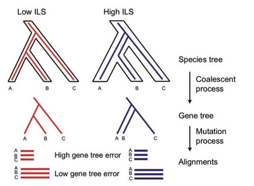
Simulation of ILS and gene tree estimation error. ILS was simulated though the coalescent process by setting low (0.01) and high (0.1) theta values. DNA alignments were subsequently generated through the mutation process based on simulated gene trees. Five alignments were generated for each gene tree with lengths of 300, 400, 500, 1000, and 1500 bp (only two are shown in the graph). Shorter alignment lengths increase in gene tree estimation error.
In order to assess the sensitivity of our simulation results to the choice of input species tree and theta values, we additionally examined gene tree–species tree discordance among bootstrapped samples. We simulated 1500 gene trees for each of the 100 MP-EST bootstrapped species trees. Gene trees were simulated directly from each species tree using the “sim.coal.mpest” function in the R package Phybase (Liu and Yu 2010). This method does not require a priori theta parameters as was imposed in our simulation above and so alleviates concerns of applying erroneous theta values. We subsequently quantified the gene tree–species tree discordance for each bootstrap replicate as described above. We did not use these gene trees to simulate alignments because these gene trees are ultrametric (Liu and Yu 2010) and thus not suitable for such purpose.
A Test of Deviation from the MSC Model Using Triplet Frequencies
We provide a brief overview of a triplet frequency based method we developed to detect gene flow in the presence of ILS. The theory behind the model and assessments of statistical power can be found in Meng and Kubatko (2009). The logic of this test is similar to the |$D$|-statistic (Green et al. 2010; Durand et al. 2011), but gene tree topology is used instead of site patterns to mitigate mutational noise in highly divergent lineages. Our script for applying this methodology is available on Github (http://github.com/lmcai/Coalescent_simulation_and_gene_flow_detection).
Consider a rooted three-taxon species tree (Fig. 2a): under the coalescent model, gene trees arising within the species tree have three distinct topological outcomes. The two minor discordant triplets will occur at equal frequency, which is |$\frac{1}{3}e^{-t}$| with |$t$| being the internal branch length in coalescent units (Fig. 2a). Gene flow between nonsister taxa, however, will lead to asymmetry in the minor triplet frequencies due to exchanging alleles. The difference between the two minor triplet frequencies can therefore be used to test for gene flow: significant deviation of the observed frequency difference from zero will reject the null hypothesis of no gene flow (Meng and Kubatko 2009).
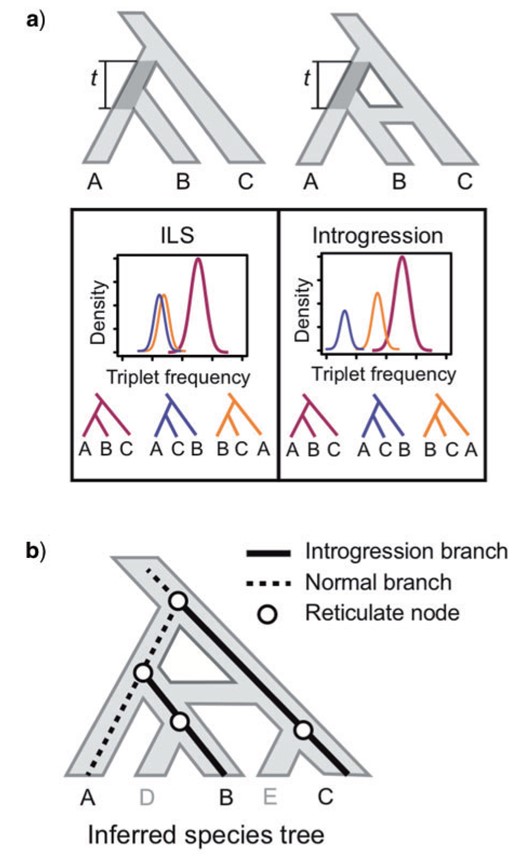
Identification of reticulate evolution using triplet frequencies. a) Theoretical expectations of triplet frequency distribution under the multi-species coalescent (MSC) model with and without introgression. In the case of incomplete lineage sorting (ILS), the frequency of two minor topologies are expected to be symmetrical (left). In the case of introgression, one of the minor topologies will occur with higher frequency due to gene flow (right). The length of the internal branch t is measured in coalescent units. b) Mapping asymmetrical triplets to species tree to identify reticulate nodes. In the triplet ((A,B),C) where gene flow is identified, the two external branches leading to species exchanging alleles (B and C) are labeled as `introgression branches’. All nodes along these two introgression branches are treated as reticulation nodes.
Z-score and Chi-square tests are often used to evaluate the statistical significance of the difference between minor topology frequencies or site patterns (e.g., Blischak et al. 2018; Pease et al. 2018). However, simulation research has demonstrated that these approaches can be confounded by ILS and random sampling error (Zheng and Janke 2018, see also Supplementary Note 1 available on Dryad). Additional variation due to missing data or mutational noise in the empirical data set may further increase the risk of false positives. We therefore propose a simulation-based method incorporating parametric bootstrapping to evaluate the statistical significance without assuming the underlying distribution of the frequency difference between the two minor triplets. Here, the observed triplet frequency is compared to a simulated null distribution using coalescent and mutational parameters estimated from the empirical data. This null distribution captures the variation arising from ILS, estimation error, sampling error, and missing data. We demonstrate via simulation that our method has lower false positive rate compared to the Z-score or Chi-square tests using site pattern or quartet topologies (Supplementary Note 1 available on Dryad). To generate the null distribution, we simulated gene trees using the “sim.coal.mpest” function in Phybase for each of the 100 BP species trees estimated from the empirical data set. This generates 100 sets of simulated gene trees, each containing the same number of loci as the empirical data set. Within each set of simulated gene trees, we then generated missing data for each species by randomly removing that species from the gene trees so that they contain the same amount of missing data as the empirical data. Finally, the null frequency distribution of each triplet is summarized across the 100 bootstrap replicates. We reject the null hypothesis if the difference between the two minor triplets in the empirical data exceeded the maximum observed in the simulated null. Such triplets significantly violate the assumptions of the MSC model, and point towards gene flow as an additional factor influencing gene tree heterogeneity, though ancestral population structure (Slatkin and Pollack 2008) and biases in substitution or gene loss can produce asymmetrical triplet as well (see Discussion below).
To apply this method to our empirical data, we first summarized the frequency distribution for all 41,664 triplets in Malpighiales using empirical gene trees inferred from our low-stringency data set (analysis No. 15 in Supplementary Table S2 available on Dryad). We then simulated null distributions using the 100 MP-EST BP species trees inferred from the same data set following the methods described above. The observed triplet frequency in the empirical data set was compared to the null distribution to determine whether there is significant deviation from the MSC model.
Identifying Hotspots of Reticulate Evolution Using the Reticulation Index
We developed a relative measurement statistic, the “Reticulation Index,” to quantify the intensity of introgression at each node. First, for each asymmetrical triplet, we identified the two species exchanging alleles based on triplet frequencies—the second most frequent triplet is caused by gene flow and the two closer-related species in this triplet are implicated in introgression (Fig. 2b). Because the timing of introgression along these two branches cannot be determined using gene tree topology alone (Edelman et al. 2019; Hibbins and Hahn 2019) and introgression affects all of the descendant nodes of the donor and recipient lineages, we then map the two introgression branches to the species tree and treat all nodes on these two branches to be involved in introgression (Fig. 2b). Finally, for each node on the species tree, we counted the number of introgression branches that were mapped to it. These raw counts were then normalized by the total number of triplets associated with that node. The resulting percentage is the Reticulation Index. This metric does not distinguish the donor versus the recipient lineage and incomplete taxon sampling may lead to the failure of introgression detection. But in theory, as long as at least one species from the recipient lineage and one from the donor lineage are sampled, the algorithm should be able to identify the signal. The script for calculating the Reticulation Index and visualizing the result on a species tree is available in the above Github repository (http://github.com/lmcai/Coalescent_simulation_and_gene_flow_detection).
A Novel Method to Quantify Gene Tree Variation Due to ILS, Gene Tree Estimation Error, and Gene Flow
Untangling the effects of ILS, gene tree estimation error, and gene flow is challenging since they all lead to gene tree–species tree discordance. Here, based on a multiple regression model (Grömping 2006), we assign shares of relative importance to ILS, gene tree estimation error, and gene flow in generating gene tree variation by variance decomposition.
For all 63 internal nodes in our species tree, we separately estimated the level of ILS, gene tree estimation error, and gene flow. ILS is represented by our estimates of theta. Gene flow is represented by the Reticulation Index for each node. To infer the level of gene tree estimation error at each node, we additionally simulated 423 gene alignments of 446 bp (median alignment length in low-stringency data set) from the MP-EST species tree, but each with unique substitution model parameters estimated from the empirical alignments. This simulation and phylogeny inference followed the same strategy of alignment simulation described above (Fig. 1). We subsequently inferred phylogenies for these alignments and summarized them on the species tree to obtain the BP value at each node. Here, the BP values represent the gene tree variation generated by estimation error.
The gene tree variation in the empirical data is obtained by summarizing bootstrap trees from each of the 423 loci in our low-stringency data set onto the species tree. The resulting BP values represented observed gene tree variation at each node. We then inferred the relative contribution of ILS, estimation error, and gene flow in explaining gene tree variation using linear regression methods implemented in the R package relaimpo (Grömping 2006). We additionally applied log transformations to the regressors to measure the goodness of fit using |$R^{2}$|. To decompose the relative importance of the three regressors, we used four different methods, “lmg,” “last,” “first,” and “Pratt” (Lindeman 1980; Pratt 1987). All are capable of dealing with correlated regressors and “lmg” is the most robust method among them (Grömping 2006). We applied the functions “boot.relimp” and “booteval.relimp” to estimate the relative importance and their confidence interval by bootstrapping 100 times. The R script for the relative importance decomposition analysis is available in the above GitHub repository (http://github.com/lmcai/Coalescent_simulation_and_gene_flow_detection).
Comparison to Other Techniques
We compared the performance of our triplet methods with three additional introgression detection methods that can be applied to large data sets, including HyDe (Blischak et al. 2018), quartetsampling (Pease et al. 2018), and PhyloNet_MPL (Yu and Nakhleh 2015). HyDe is a phylogenetic invariant method that evaluates hypotheses of introgression based on site patterns in triplets. Quartetsampling is most similar to our method and tests introgression using quartet topology frequencies. PhyloNet_MPL infers species networks using a maximum pseudolikelihood approach.
We applied the alignments, gene trees, and species tree inferred from our low-stringency data set (analysis no. 15 in Supplementary Table S2 available on Dryad) to these three methods and compared the results to our estimation. In addition, we also evaluated the false positive rate for HyDe and quartetsampling using simulation. We chose these two methods because they similarly test introgression using triplets or quartets and provide estimations of the proportion of gene flow at each internal node. But unlike our method, HyDe uses site patterns and conducts hypothesis testing using a Z-score; quartetsampling instead examines quartet topologies heuristically and conducts hypothesis testing using a Chi-square test. PhyloNet_MPL is not tested here because the network reconstructed by PhyloNet_MPL does not quantify the gene flow and the inferred network is not directly comparable to the Reticulation Index from our method (Supplementary Figs. S8–10 available on Dryad). We applied the simulated alignments based on mutational parameters inferred from our Malpighiales low-stringency data set to assess these two methods. This simulated data set reflects a scenario of high sequence divergence, high rate heterogeneity, and high phylogenetic uncertainty. Detailed description of parameter settings and input file generation for HyDe and quartetsampling analyses are provided in Supplementary Note 1 available on Dryad.
Results
Hybrid Enrichment
We successfully captured and sequenced 423 of our 491 targeted loci. The resulting data matrix was densely sampled and included only 12|$\%$| missing data. One hundred and one loci included at least 61 of the 64 species (95|$\%$| occupancy) and only four loci had more than 19 missing species (|$>$|30|$\%$|). The locus sampling per taxon varied from 423 (Leea guineense) to 278 (Ouratea sp. and Lophopyxis maingayi). After applying site-subsampling, the alignment lengths ranged from 190 to 885 bp (median 446 bp) for the low-stringency data set, 157 to 791 bp (median 376 bp) for the medium-stringency data set, and 112 to 751 bp (median 271 bp) for the high-stringency data set (Supplementary Table S4 available on Dryad). The low-stringency data set has the highest proportion of flanking regions (on average 26.2 |$\%$| of the aligned sites) and the high-stringency data set contains almost no flanking regions because the average length of the alignment is shorter than the average of the probe regions (303 bp vs. 343 bp; Buddenhagen et al. 2016). In all data sets, the number of parsimony informative sites and the average nodal support was significantly positively correlated with alignment length (|$P$|-value |$<$|1e-5, Fig. S1). Sequence alignments and supplementary materials are available on Dryad (http://doi.org/10.5061/dryad.hx3ffbgck).
Flanking Regions Increase Gene Tree and Species Tree Support
We observed increasing mean BP support among gene trees as increasingly larger percentages of the flanking region were included. The average gene tree nodal support from our low-stringency data set (42 ML BP) was significantly higher than nodal support estimates for the medium (39 ML BP, |$P$|-value |$=$| 1.2e–89 in paired t-test) and high-stringency data sets (35 ML BP, |$P$|-value |$=$| 1.3e–77, Supplementary Fig. S2a available on Dryad).
These increases in gene tree support also contributed to increased species tree support as well as species tree inference congruency. For both concatenation and coalescent analyses, species trees estimated from the low-stringency data set with highest amount of flanking regions, always resulted in the highest average BP support (Supplementary Fig. S2b,c, Table S2 available on Dryad) and the lowest pairwise RF distances (Supplementary Fig. S2d available on Dryad) indicating increased statistical consistency when adding flanking regions.
Malpighiales Species Tree Support
We observed significantly higher average species tree nodal support in concatenation compared to coalescent reconstructions (Supplementary Table S2 available on Dryad, |$P$|-value |$=$| 2.62e-28 in paired |$t$|-test). However, our results also suggest statistical inconsistency across data sets when applying concatenation because the pairwise weighted Robinson–Foulds distance (WRF) is higher among species trees inferred from concatenation methods (Supplementary Fig. S3 available on Dryad). High WRF indicates more well-supported topological conflicts and further supports mounting evidence that coalescent methods are more consistent when reconstructing species tree relationships involving extensive ILS (i.e., the anomaly zone, Degnan and Rosenberg 2006, Rosenberg and Tao 2008). In addition, we did not find locus subsampling based on locus length, number of PI sites, or gene tree quality help to increase species tree support or consistency (Supplementary Note 2, Table S2 available on Dryad). Neither did collapsing poorly supported nodes in gene trees improve species tree estimation for the coalescent-based method (Supplementary Note 3 available on Dryad).
Our best-supported species trees inferred with ASTRAL and MP-EST uncovered ten major subclades of Malpighiales (Clade 1 to 10 in Fig. 3). These relationships corresponded to families or closely related clades of families, five of which have previously been identified using plastid genome (Fig. 3, Xi et al. 2012). Five new clades were supported with |$ \ge $|50 BP, |$>$|0.90 PP. Three of these newly identified clades are in conflict (|$>$|70 BP) with the plastid phylogeny from Xi et al. (2012) and are discussed more extensively below. Interrelationships among these ten major subclades, however, were not well supported (|$<$|50 BP).
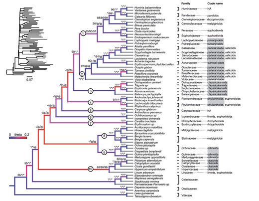
Species phylogeny of Malpighiales derived from MP-EST with complete low-stringency data set (analysis No. 15 in Table S2). Gene trees are estimated using MrBayes. Branches are colored by the inferred population mutation parameter theta. Warmer colors indicate higher theta and thus higher level of ILS. Terminal branches are colored grey due to lack of data to infer theta. BP values from best-supported MPEST/ ASTRAL/RAxML analyses (analysis No. 15, 17, and 11 in Table S2) are indicated above each branch; an asterisk indicates 100 BP support; a hyphen indicates less than 50 BP; an ‘@’ symbol indicates an alternative topology. Branch lengths estimated from RAxML by fixing the species tree topology are presented at the upper left corner. The eleven major clades highlighted in the discussion are identified with circled numbers along each relevant branch. The clade affiliation for each family based on the plastid phylogeny (Xi et al. 2012) is indicated on the right. Clades identified by Xi et al. (2012) that are also monophyletic in this study are highlighted using grey shades.
Simulated Levels of ILS and Gene Tree Estimation Error Reflects Empirical Data
The 5|$\%$| and 95|$\%$| quantiles of theta were inferred to be 0.0254 and 0.176, respectively, with a median of 0.0688. Nodes with high values of theta were mostly found along the backbone of the species tree, indicating extensive ILS within this region of the tree (Fig. 3). This is likely an overestimation of theta since all topological variations are attributed to coalescent process, including the ones originate from mutational variance (Huang and Knowles 2009). We therefore set the theta parameter to be 0.01 and 0.1 in our coalescent gene tree simulation, which reflected the left and right tails of low and high ILS estimated from empirical data.
In our simulation, the average gene tree estimation error was 0.319 for alignments of 300 bp, 0.261 for 400 bp, 0.221 for 500 bp, 0.133 for 1000 bp, and 0.098 for 1500 bp under low ILS and 0.340 for alignments of 300 bp, 0.286 for 400 bp, 0.241 for 500 bp, 0.161 for 1000 bp and 0.120 for 1500 bp under high ILS. Here, an RF distance of 0 signifies error-free reconstruction versus 1 indicating that none of the true nodes are recovered. Gene tree estimation error was therefore lower in low ILS (|$P$|-value |$=$| 6.08e-16 in Student’s |$t$|-test), but was still significantly higher than that estimated from empirical data (|$P$|-value |$=$| 4.24e-65 in Student’s |$t$|-test; see Supplementary Note 2, Fig. S4 available on Dryad).
Simulation Yields Consistent and Accurate Species Tree Estimation
In our empirical analyses, the low-stringency data set yielded the lowest average gene tree–species tree conflict of 0.563 among the other data sets. In our simulations, the highest average gene tree–species tree conflict observed was 0.507, by setting theta = 0.1 and alignment length = 300 bp. Therefore the lowest empirical gene tree–species tree discordance was still significantly higher than the simulated conditions with extremely high levels of ILS and gene tree estimation error (|$P$|-value |$=$| 2.2e-16, Student’s |$t$|-test, Fig. 4a). The same conclusion also applies when simulating gene trees directly from the species tree without setting theta a priori (Fig. 4b).
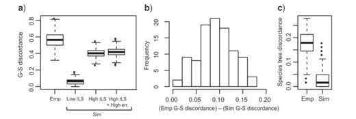
Extensive gene tree discordance in empirical versus simulated data. a) Gene tree–species tree (G–S) discordance in the empirical (Emp) and simulated (Sim) data assuming fixed theta in simulation. Discordance is measured by RF distance between inferred gene trees and the species tree. Under various simulated conditions of ILS (e.g., `Low ILS’, theta |$=$| 0.01 and `High ILS’, theta |$=$| 0.1) and gene tree estimation error (`High ILS |$+$| High err.’, theta |$=$| 0.1, alignment length|$=$|300 bp), the simulated gene tree–species tree discordance is significantly lower than that from empirical data. b) Gene tree–species tree discordance is higher in empirical versus simulated conditions without setting theta a priori. For each BP data set, gene tree–species tree discordance is measured and compared in both empirical and simulated data sets. Positive values indicate higher gene tree–species tree discordance in our empirical data. c) Species tree estimation discordance in empirical data (left) and simulated data (right).
Moreover, even under the simulated conditions of extremely high ILS and gene tree estimation error, both concatenation and coalescent-based methods yielded consistent and accurate species tree estimation (Fig. 4c, Supplementary Fig. S5 available on Dryad). For both methods, no more than 12 nodes fail to be recovered (RF distance |$=$| 0.10 to the true species tree, Supplementary Fig. S5 available on Dryad) even using the smallest data set (100 loci with 300 bp in length). The performance of coalescent-based methods is mainly affected by gene tree estimation error (Supplementary Fig. S5 available on Dryad). Under the highest gene tree estimation error (alignment length |$=$| 300 bp), both ASTRAL and MP-EST require 1000 loci to recover the true species tree. For concatenation methods, ML estimations are robust under low ILS levels, which is consistent with previous findings (Mirarab et al. 2014b; Tonini et al. 2015). We were able to recover the correct species tree with the smallest data set (100 loci with 300 bp in length) under low ILS (theta |$=$| 0.01). However, major challenges and inaccurate species trees are generated under high ILS. Under such conditions, it requires the largest data set (1500 loci with |$ \ge $|400 bp length) to recover the true species tree (Supplementary Fig. S5 available on Dryad).
Relative Contribution of ILS, Gene Tree Estimation Error, and Gene Flow to Gene Tree Variation
Among all 41,664 triplets we examined, 553 (1.3|$\%$|) have significant asymmetrical minor frequencies. The node with the highest Reticulation Index is the MRCA of Clade 1 and Clade 2 (the MRCA of Salicaceae and Euphorbiaceae; Fig. 5c). 10.3|$\%$| of the triplets associated with this node are significantly asymmetrical. According to our relative importance decomposition analysis, ILS, gene tree estimation error, and gene flow explain 66.9|$\%$| of the total gene trees variation across all internal nodes using the lmg algorithm (|$R^{2} = 0.669$|). Gene tree estimation error is the most dominant factor, which explains 34.8|$\%$| of the gene tree variation (Supplementary Fig. S6 available on Dryad). The second most significant factor is gene flow, which explains 21.4|$\%$| of the gene tree variation. And ILS explains the least variation (10.0|$\%$|). The relative ranks of these three factors are consistent among regression methods and bootstrap replicates (Supplementary Fig. S6 available on Dryad).
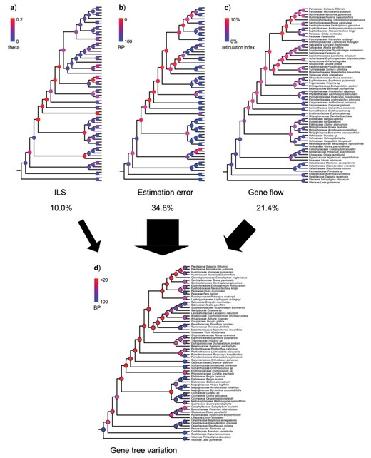
Relative contributions of ILS, estimation error, and gene flow across Malpighiales. a) ILS. Nodes are colored by inferred population mutation parameter theta. b) Gene tree estimation error. Nodes are colored by BP values, which represent percentage of recovered nodes from simulation (see Materials and Methods section). c) Gene flow. Nodes are colored by Reticulation Index. d) Gene tree variation. Nodal BPs reflect nodal recovery in gene trees. Percentages of gene tree variation ascribed to ILS, estimation error, and gene flow are indicated by black arrows.
Further investigation revealed significant negative correlation (|$P$|-value 2.2e-16) between the overall gene tree variation and species tree support (Supplementary Fig. S7a available on Dryad). All of the contributors to gene tree variation—ILS, tree estimation error, and introgression—are strongly negatively correlated with species tree support (|$P-$|value |$<$|6.6e-4, Supplementary Fig. S7b–d available on Dryad). We observed the highest level of ILS, introgression and gene tree estimation error for the most recalcitrant nodes along the backbone of the phylogeny using our methods (Supplementary Fig. S7b–d available on Dryad). This further corroborates our conclusion that a combination of all three factors contribute to this low support. We did not find significant correlation between the estimated level of introgression and ILS, suggesting that our triplet method can effectively distinguish these two phenomena. However, both ILS and introgression are positively correlated to gene tree estimation error (|$P$|-value |$<$| 6.8e-3).
Our Triplet Method has Lower False Positive Rates Compared to Other Approaches
The application of the empirical data set from Malpighiales to three alternative introgression identification methods resulted in varied performance. Regardless, these alternative methods produced inferior results to our method under simulation. The network inference implemented in PhyloNet_MPL generated inconsistent estimations among independent runs when setting the number of reticulation events to be one, two, and three (Supplementary Figs. S8–10 available on Dryad). The network with two reticulate branches received highest likelihood (log probability |$-$|1.0598e-7), but one Malpighiales lineage (the MRCA of Phyllanthaceae and Picrodendraceae) was placed with the distantly related outgroup Vitales and inferred to exchange alleles with Ixonanthaceae (Malpighiales). These results highlight the challenges of network reconstruction when phylogenetic uncertainty is high.
For HyDe and quartetsampling, we applied both the empirical and simulated data set and compared their performance with our method. The site pattern-based HyDe identified gene flow in 394 triplets (1.3|$\%$|, Bonferroni corrected |$P$|-value |$1.71 \times 10^{-6})$| in the empirical data set, but identified even more (|$n = 2417$|, 8.2|$\%$|) in the simulated, gene-flow-free data set of the same size. Moreover, in both the empirical and simulated data, these outlier triplets are randomly distributed across the phylogeny (Supplementary Figs. S11 and S12 available on Dryad). Such random distribution is inconsistent with the pattern created by gene flow in which the donor and recipient lineages are expected to be overrepresented in these triplets. These results indicate that the accuracy of HyDe is likely compromised by mutational noise and does not provide meaningful inference of gene flow for highly divergent species. On the other hand, the topology-based quartetsampling yielded more consistent estimations of gene flow when compared to our method. For the empirical data set, significant deviation from the coalescent model was identified in 15 nodes. Eight of these nodes are located within Clades 1 and 2 (Supplementary Fig. S13 available on Dryad), which is consistent with our findings (Fig. 5c). However, quartetsampling also reported false positives in 7 out of the 62 (11.3|$\%$|) internal nodes (Chi-square test |$P$|-value |$<$|0.05) when applying the simulated data. The majority of these false positives were localized along the backbone of the phylogeny (Supplementary Fig. S14 available on Dryad), suggesting that this method is sensitive to species tree estimation error and phylogenetic uncertainty. In contrast, our triplet method does not use species tree topology when evaluating gene flow. It is thus more robust under high phylogenetic uncertainty. In addition, our method reports none of these false positives because the simulated data itself is used to assess deviation from the coalescent model using parametric bootstrapping.
Discussion
Our results indicate that despite extensive phylogenomic data, the early branching order of Malpighiales remains uncertain. We attribute this to a combination of factors—a perfect storm—involving ILS, gene tree estimation error, and gene flow. Below, we highlight our findings in four subsections: the phylogenetic utility of flanking regions in sequence capture data, novel phylogenetic relationships gleaned for Malpighiales, an efficient method to investigate gene flow in large data sets, and a novel simulation-based method to decompose gene tree variation into various contributing factors.
Flanking Regions Greatly Enhance Phylogenetic Resolution
Hybrid enrichment probes are designed to capture highly conserved anchor regions as well as the more variable flanking regions adjacent to these anchors. Despite the perceived utility of these flanking regions in mammals (Mallet 2007) and more recently in in plants (Fragoso-Martínez et al. 2017), assumptions of the enhanced phylogenetic utility of these flanking regions have not been tested explicitly to our knowledge. Here, we observed significantly higher average ML BP across gene trees, increased species tree support, and most importantly, increased species tree estimation congruency as flanking regions were increasingly added (Supplementary Fig. S2 available on Dryad). This suggests that longer loci, favoring more phylogenetically informative flanking regions, should be prioritized in future anchored hybrid enrichment kit designs. These flanking regions represent genomic regions under nearly neutral selection where mutation rates are high, and thus appear to be a rich source of phylogenetic utility. It has been demonstrated that the inclusion of genes with higher mutation rates can greatly enhance phylogenetic resolution, even deep within organismal phylogenies (Hilu et al. 2003; Lanier et al. 2014). Our site-subsampling strategy, which includes increasingly larger proportions of these more rapidly evolving flanking regions provides the first empirical evidence that these regions are particularly informative for resolving phylogenetic relationships at shallow and deeper phylogenetic depths.
Sequence Capture Data Confirms Malpighiales Relationships and Identifies Novel Clades
We assessed the performance of hybrid enrichment markers by evaluating support for major clades previously identified from plastome sequences (Xi et al. 2012; Fig. 3). The majority of the well-supported (|$>$|90 BP) clades identified by Xi et al. (2012) are corroborated in our analyses with high confidence (|$>$|97 BP). These include the parietal, clusioid, phyllanthoid, ochnoid, chrysobalanoid, and putranjivoid subclades. With rare exception, relationships within these clades were also identical to those by Xi et al. (2012). In the case of the parietal and clusioid clades, internal relationships were less well supported owing to conflicting topologies recovered among coalescent and concatenation methods (low nodal support indicated by `–’ in Fig. 3). Within the parietal clade, for example, the monophyly of the salicoids sensuXi et al. (2012), Fig. 3 is supported by the RAxML phylogeny with moderate support (69 BP) but is not supported in any of the coalescent methods.
Additionally, we discovered several noteworthy clades that conflict with those reported by Xi et al. (2012). The euphorbioids, malpighioids, and rhizophoroids were paraphyletic in all of the best-supported MP-EST, ASTRAL, and RAxML analyses (Fig. 3). The euphorbioids—including Euphorbiaceae, Peraceae, Lophopyxidaceae, Linaceae, and Ixonanthaceae—were split into four polyphyletic groups. In particular, Linaceae was placed as sister to the clusioid clade in all of the best-supported coalescent and concatenation analyses (Fig. 3). The affiliation of Linaceae to the clusioids instead of to other members of the euphorbioids is also supported in a recent transcriptomic study of this group with less dense taxon sampling (Cai et al. 2019). Within malpighioids, Centroplacaceae is confidently placed (|$>$|86 BP) with Humiriaceae, Pandaceae, and Ctenolophonaceae (Fig. 3) instead of with Malpighiaceae and Elatinaceae. This relationship is partially supported by Wurdack et al. (2004) in which Centroplacaceae was placed with Pandaceae, although with low support. Within the rhizophoroids, Ctenolophonaceae was well nested (|$>$|98 BP for coalescent methods) within a clade including Euphorbiaceae and Pandaceae (Clade1 in Fig. 3) rather than with Rhizophoraceae and Erythroxylaceae.
ILS and Gene Tree Estimation Error Alone Are Insufficient to Explain the Lack of Species Tree Support in Malpighiales
Our simulations to explore gene tree heterogeneity encompass the full distributional range of ILS and gene tree estimation error inferred from the empirical data, and clearly demonstrate that the data we have assembled should be sufficient to resolve Malpighiales species tree relationships. Specifically, despite our inability to estimate a well-supported species tree from our empirical data, we were able to recover a species tree with very high confidence in simulation (mean nodal support |$>$|91 BP). This is true even when ILS (theta |$=$| 0.1) and gene tree estimation error (alignment length |$=$| 300 bp) were set to the highest levels inferred from our empirical data. Such extreme levels of theta, in particular, are ten times higher than empirical estimations from Arabidopsis and Drosophila (0.01–0.001 in both cases; Drost and Lee 1995; Fischer et al. 2017). Even when down sampling our data set under these extreme conditions to include a mere 100 loci, the RF distance between the true species tree and the estimated species trees is no more than 0.1 (Supplementary Fig. S5 available on Dryad). In addition, we observed far fewer conflicts among species trees reconstructed from different methods and data partitions in simulation versus from those estimated from the empirical data (Fig. 4c). These results suggest that ILS and gene tree estimation error alone are insufficient to explain the lack of resolution along the spine of Malpighiales and suggest that additional factors likely contribute to gene tree heterogeneity.
Gene Flow Compromises Malpighiales Species Tree Resolution: A Novel Method for Assessing Gene Tree Heterogeneity
Beyond ILS and gene tree estimation error, gene tree heterogeneity is also attributable to two other common biological factors: gene duplication and gene flow (Yang 2006). As we demonstrate above, the first two factors alone are insufficient to explain this lack of resolution. Orthology assignment problems owing to gene duplications are also highly unlikely for two reasons. First, our sequence capture data set was specifically designed for single-copy nuclear loci across land plants (Buddenhagen et al. 2016). Second, large-scale genome duplication identified in Malpighiales all occurred subsequent to the explosive radiation where discordance is localized (Cai et al. 2019). Thus, biased gene loss arising from genome duplications are unlikely to hinder our ability to resolve backbone relationships in the order. Additional analytical artifacts not reflected in our assessment include homolog calls, alignment error, and most importantly, misspecification of DNA substitution models, all of which can compromise species tree estimation. Though these analytical errors may explain some discordance, it is quite possible that conflicts are attributed to additional biological phenomena.
It is estimated that at least 25|$\%$| of plant species and 10|$\%$| of animal species hybridize (Mallet 2007). Various phylogenetic network and phylogenetic invariant methods have been developed to assess gene flow (Elworth et al. 2019). These methods have provided valuable insights into reticulate evolution, including those associated with the rapid radiations in wild tomatoes and heliconius butterflies (Pease et al. 2016; Elworth et al. 2019). However, phylogenetic network inference using full likelihood under the multispecies network coalescent model can only be applied to networks involving fewer than 10 taxa and three reticulations (Yu and Nakhleh 2015; Elworth et al. 2019). Pseudolikelihood based network inference can be scaled to larger data sets, but the application of this method to our data yielded inconsistent inferences when different numbers of reticulation branches were set a priori. On the other hand, the performance of the phylogenetic invariant methods, including the |$D$|-statistic, HyDe, and D|$_{\rm Foil}$|, has only been rigorously tested in recently diverged lineages (Pease and Hahn 2015; Zheng and Janke 2018). We demonstrated through simulation that HyDe was sensitive to mutational noise (Supplementary Note 1 available on Dryad), which was similarly concluded for the |$D$|-statistic by Blair and Ané (2020). The topology-based quartetsampling mitigated some of the limitations of the phylogenetic invariant methods when investigating highly divergent lineages. It generated the most consistent results when compared to our method (Fig. 5c and Supplementary Fig. S13 available on Dryad), but it also had a high false positive rate of 11.3|$\%$| when analyzing the simulated data. On the contrary, our triplet method uses simulation-based hypothesis testing and did not yield false positive results. In addition, the Reticulation Index we proposed identifies hotspots of reticulate evolution by summarizing the proportion of significantly asymmetrical triplets associated with each node. Unlike the widely used concordance factor (Baum 2007) or similar metric implemented in quartetsampling (quartet differentiation, Pease et al. 2018), which calculates the ratio of concordant and discordant gene trees and only provides a Boolean test of coalescent model fitness, our Reticulation Index provides a quantitative measure of gene flow across the species tree. In summary, our triplet method offers an efficient and conservative assessment of reticulate evolution in large clades and in deep time despite high phylogenetic uncertainty.
In Malpighiales, the Reticulation Indices are especially high in deeper parts of the phylogeny, suggesting that certain clades may contribute substantially to this phenomenon (Fig. 5c). In particular, we hypothesize that the overabundance of asymmetrical triplets observed within Clades 1 (MRCA of Euphorbiaceae and Putranjivaceae) and Clade 2 (MRCA of Salicaceae and Violaceae) result from ancient and persistent gene flow between early diverging members of these lineages. This result is also confirmed by examining quartet frequencies using quartetsampling (Supplementary Fig. S13 available on Dryad). Specifically, Clade 1 contains six paralogous lineages from the plastid phylogeny (Xi et al. 2012) and is a major hotspot for plastid-nuclear conflict. Such conflict is widely recognized as an indicator of introgression (Soltis and Kuzoff 1995; Baum et al. 1998). Moreover, members of two clades, the putranjivoids and Pandaceae, have previously been implicated in the top three most unstable nodes of all angiosperms (Smith et al. 2013). We hypothesize that this may be attributed to the chimeric nature of their ancestral genealogy resulting from gene flow. The Reticulation Index is also significantly negatively correlated with species tree support (Supplementary Fig. S7d available on Dryad), suggesting that introgression is an important barrier for robust species tree estimation in Malpighiales. For example, among the most recalcitrant nodes where almost no bootstrap replicates recover the same topology, we also observed the highest values of inferred introgression. Moreover, we observed no correlation between the estimated level of ILS and introgression, suggesting that our methods can effectively distinguish these two phenomena. However, nodes with strong introgression signals also have higher gene tree estimation error (Supplementary Fig. S7e available on Dryad). One possible explanation for such correlation is that the short branch lengths created by introgression (Leaché et al. 2014) may lead to elevated estimation error at these nodes.
To better characterize gene tree variation attributable to ILS, gene tree estimation error and gene flow, we devised a novel method to parse variations attributable to these analytical and biological factors using regression models. This distinguishes the contribution of evolutionary forces to those arising from analytical errors. Our method revealed that the majority of variation is due to estimation error (34.8|$\%$|), while gene flow and ILS account for 21.4|$\%$| and 10.0|$\%$|, respectively. This decomposition analysis is based on estimations of ILS, gene tree error, and gene flow through simulation and is subject to common limitations of regression analyses. As a result, errors from the simulation and regression analysis can render the absolute values of these percentages less reliable. Regardless, the relative influence of biological and analytical aspects of gene tree variation as interpreted from these metrics can shed important light on empirical investigations and the development of enhanced species tree inference methods. For example, though gene tree error is to blame for the majority of gene tree variation in our test case, gene flow still plays a significant role in gene tree variation. Therefore, a species network inference method that accommodates gene flow is essential to better understand the early evolutionary history of Malpighiales. Application of this method to other taxonomic groups will also reveal the key factors contributing to recalcitrant relationships and provide guidance for phylogenomic marker design targeting at specific questions.
Our results suggest that a confluence of factors—ILS, gene tree estimation error, and gene flow—influence this lack of resolution and contribute to a perfect storm inhibiting our ability to reconstruct branching order along the backbone of the Malpighiales phylogeny. Gene flow, in particular, is a potentially potent, and overlooked factor accounting for this phenomenon. Despite a relatively small percentage of asymmetrical triplets attributed to gene flow (1.3|$\%$| of all triplets), they appear to contribute substantially to gene tree heterogeneity based on our relative importance decomposition (21.4|$\%$|). Our approach of interrogating this phenomenon using triplet frequencies and the relative importance analyses can elucidate factors that give rise to gene tree variation. These approaches are likely to be especially useful for investigating the causes of recalcitrant relationships, especially at deeper phylogenetic nodes, and to highlight instances where relationships are better modeled as a network rather than a bifurcating tree.
Supplementary Material
Data available from the Dryad Digital Repository: http://doi.org/10.5061/dryad.hx3ffbgck.
Funding
Funding for this study came from Harvard University, and US National Science Foundation Assembling the Tree of Life Grant 9DEB-0622764 and from DEB-1120243 and DEB-1355064 to C.C.D.).
Acknowledgments
We would like to thank Sean Holland and Michelle Kortyna at the Florida State University Center for Anchored Phylogenomics for their assistance with data collection and analysis. We would like to thank Scott Edwards and Davis Lab members for helpful comments.
References
Arabidopsis Genome Initiative.
