


Abstract
Individuals befriend others who are similar to them. One important source of similarity in relationships is similarity in felt emotion. In the present study, we used novel methods to assess whether greater similarity in the multivoxel brain representation of affective stimuli was associated with adolescents’ proximity within real-world school-based social networks. We examined dyad-level neural similarity within a set of brain regions associated with the representation of affect including the ventromedial prefrontal cortex (vmPFC), amygdala, insula, and temporal pole. Greater proximity was associated with greater vmPFC neural similarity during pleasant and neutral experiences. Moreover, we used unsupervised clustering on social networks to identify groups of friends and observed that individuals from the same (versus different) friend groups were more likely to have greater vmPFC neural similarity during pleasant and negative experiences. These findings suggest that similarity in the multivoxel brain representation of affect may play an important role in adolescent friendships.
It is an old adage that “birds of a feather flock together.” Decades of research bear out that people initiate and maintain friendships with those who are similar to them (McPherson et al. 2001, Rivera et al. 2010). Such “homophily” (Lazarsfeld and Merton 1954) is observed as similarity in friends’ demographic ascriptions (e.g. race/ethnicity, sex, and age), achievements, (e.g. education and occupation), personality (e.g. extraversion), emotional profiles (e.g. levels of happiness and depressive symptomatology), values (e.g. religion and political orientation), behaviors (e.g. engagement in prosocial or health risk behaviors), and even genotype (McPherson et al. 2001, Fowler et al. 2011, van Workum et al. 2013, Christakis and Fowler 2014, Jin and Zafarani 2017). Psychologically, homophily may emerge from humans’ greater attention to (Symons and Johnson 1997, Patterson and Joseph 2013) and positive regard for (Taylor and Brown 1988) self-relevant attributes.
Recent evidence reveals a possible mechanism of homophily: friends seem to possess shared worldviews (Stephens et al. 2010, Lahnakoski et al. 2014, Parkinson et al. 2018, Nguyen et al. 2019, Higgins et al. 2021, Baek and Parkinson 2022), such that friends interpret the world in similar ways, which may make friends’ behaviors more familiar and likable (Zajonc 1968). This notion is supported by recent neuroscientific evidence. For example, young adults who are closer within a college social network demonstrate more similar patterns of neural responding to movie clips compared to individuals who are further apart (Parkinson et al. 2018, Hyon et al. 2020a, Baek et al. 2022). Importantly, experimental manipulation of dyad members’ interpretations of stories induces greater neural similarity between those individuals (Lahnakoski et al. 2014, Yeshurun et al. 2017), suggesting that neural similarity is indeed an index of shared worldview. Even in the absence of external stimuli, functional brain connectivity at rest appears to covary with social network proximity within members of an entire village (Hyon et al. 2020b), perhaps because people engage in similar autobiographical and emotional processing (Andrews-Hanna et al. 2010). Insofar as affective responding is central to how one sees the world around them (Zadra and Clore 2011), these findings collectively hint at the role of shared affective experiences as a key ingredient underlying the effects of shared worldview on friendships.
The present work examines the extent to which neural similarity during affective experiences such as pleasure and displeasure is associated with friendship in an adolescent social network. Affect is central to human conscious experience (Barrett and Bliss-Moreau 2009) and serves as a form of “glue” that can make or break relationships (Abbott et al. 1984, Graham et al. 2008, Gregory et al. 2020). Affective experience is likely to be especially important to relationships during adolescence when social and affective brain anatomy is undergoing rapid development (Blakemore and Mills 2014). At this time, affective experiences become correspondingly more frequent, intense, and volatile (Bailen et al. 2019), and peers take on increased importance (Nelson et al. 2016). We thus predicted that neural similarity during induced affective states would be associated with proximity within adolescents’ school-based social network. There is behavioral evidence that adolescents who share levels of happiness (van Workum et al. 2013) and depression (Prinstein 2007) are more likely to be friends than those with disparate levels of affective experience. Yet the behavioral evidence does not weigh in on the neurocognitive mechanisms of such adolescent homophily. Neuroscience evidence has the capacity to weigh in on the neurocognitive mechanisms underlying homophily by revealing whether neural similarity in brain regions associated with different functions is uniquely associated with friendship. For instance, greater neural similarity between friends within regions associated with affective meaning-making, such as the ventromedial prefrontal cortex (vmPFC) or temporal pole, might suggest that adolescents who are friends are more likely to interpret affective stimuli in the same way. In contrast, greater neural similarity within regions associated with salience detection and affective reactivity between friends, such as the amygdala or insula, might suggest that adolescents who are friends are more likely to have similar levels of affective reactivity. Finally, greater neural similarity within regions associated with visual processing between friends might merely suggest that friends dedicate similar levels of visual attention to affective stimuli.
To address these hypotheses, we analyzed social network data from 935 seventh and eighth graders recruited from three rural public middle schools in the southern USA between November 2017 and December 2017. These teens were asked to nominate their best and closest friends in their school and grade. From these nominations, we computed social networks retaining only instances where two teens nominated one another (i.e. reciprocal ties). Unique dyads were assigned a proximity score (ranging from 1 to 7), representing their closeness within their social network (i.e. their geodesic distance). Of our full sample, 92 participants also completed an affective pictures task during functional magnetic resonance imaging (fMRI), which allowed us to assess how their brain uniquely represented affective experiences. During this task, participants viewed pleasant, unpleasant, and neutral images in random order and were told to focus on how each picture made them feel. In a set of preregistered analyses, we then used a multivariate analytic approach to compute the pairwise similarity in dyad members’ multivoxel activation patterns across affective conditions in a given brain region. To the extent that these multivoxel response patterns approximate the psychological state subserved by a given brain region, these similarity measures may provide insight into the role of affective states in adolescent homophily (Hyon et al. 2020b). We specifically focused on activation patterns within brain regions previously implicated in the computation of affective valence (vmPFC and temporal pole) and the representation of affective salience (bilateral amygdala and anterior insula) since we reasoned that these would be key to representing individual differences in affective experiences (Kober et al. 2008, Lindquist et al. 2012, 2016). We also looked at multivoxel similarity within the primary visual cortex as a control region. Given that participants were looking at visual stimuli, we might expect neural similarity in visual cortex. However, we hypothesized that neural similarity in visual cortex would not covary meaningfully with friendship. This method allowed us to examine whether adolescents’ social proximity within real-world friendship networks significantly predicted similarity in how their brains represent affective experiences.
Finally, we conducted exploratory analyses to examine whether individuals within the same friend group, as established by data-driven classification of clusters within each school and grade-based social network, had greater neural similarity in regions of interest compared to individuals in different friend groups. We used a cluster-based approach to inductively identify friend groups as sets of individuals that were highly interconnected with each other but who had fewer connections with other individuals in the network. These novel analyses allowed us to examine whether not only individual friendships but also adolescents’ broader friendship group membership were associated with how their brains represent affective experiences. These analyses thus extended past work on neural similarity in friendship dyads to intergroup processes.
Methods
Ethical compliance
This study was approved by the University of North Carolina at Chapel Hill’s institutional ethical review board and has complied with all relevant ethical regulations. Informed consent was obtained from all adolescent participants and their parents.
Participants
Participants were recruited from three rural public middle schools in the southeast USA (N = 1385) as part of a 5-year longitudinal study. fMRI data were collected between November 2016 and September 2017, and sociometric nominations were obtained between November 2017 and December 2017 when participants were in the seventh and eighth grades. The average time elapsed between sessions was 190 days (SD = 76.98, min = 76, and max = 366).
A total of 1385 6th and 7th graders and their parents were invited to participate in this study, and 76.4% (n= 1059) of families returned consent forms. Of these families, 88.3% (n = 935) of parents consented for their child to participate in yearly data collection. Of these 935 original participants, a random selection of 284 (30.3%) was screened and invited to participate in a concurrent fMRI study. Ninety-one participants were ineligible due to learning disabilities, braces, head trauma, or other MRI contraindications, and 45 were eligible but did not participate because of scheduling difficulties or lack of interest, leaving a final sample of 148. Of these 148 participants who completed this scan session, 129 (87%) had complete sociometric and scan data. These participants were spread across schools and grades. Individuals who were not connected to their social network (i.e. because they had no reciprocated friendship nominations) were excluded from analyses, giving a final sample size of 92 individuals (Mage = 13.77 and SDage = 0.52). Demographics for this sample can be seen in Table 1. All analyses were run at the dyad level (n = 749).
Demographics for final sample (n = 92).
| Variable | n (%) | |
|---|---|---|
| Race | White Non-Hispanic or Latino/a/x | 28 (30) |
| White Hispanic or Latino/a/x | 11 (12) | |
| Hispanic or Latin/o/a/x (race unknown) | 13 (14) | |
| Black or African American Non-Hispanic or Latino/a/x | 25 (27) | |
| Multi-Racial Non-Hispanic or Latino/a/x | 9 (10) | |
| Other | 6 (7) | |
| Gender | Female | 49 (53) |
| Male | 40 (43) | |
| Unknown | 3 (3) | |
| Household income | $0—$14 999 | 7 (8) |
| $15 000—$29 999 | 16 (17) | |
| $30 000—$44 999 | 14 (15) | |
| $45 000—$59 999 | 15 (16) | |
| $60 000—$74 999 | 9 (10) | |
| $75 000—$89 999 | 1 (1) | |
| $90 000—$99 999 | 4 (4) | |
| $100 000—$119 999 | 3 (3) | |
| $120 000—$150 000 | 2 (2) | |
| $150 000+ | 4 (4) | |
| Unknown | 17 (18) |
Notes: At the time of data collection, participants were provided a number of racial and ethnic identities and asked to endorse “all that apply.” Some people selected both a canonical racial identity (e.g. “White”) and a canonical ethnic identity (e.g. “Hispanic or Latin/o/a/x”), whereas others just selected one or the other. If a person did not select “Hispanic or Latin/o/a/x,” we inferred that they were “Not Hispanic or Latin/o/a/x.” However, if a person selected “Hispanic or Latin/o/a/x” and no other category, we did not infer another racial identity. For this sample, there was complete agreement between reports of sex assigned at birth and gender. Household income was collected via parent report.
Procedure
Social network characterization
Participants were provided with a list of grade-mates (i.e. their grade roster) and asked, “Who are your best, closest friends? Choose only the students who are most important to you. Do not include ‘acquaintances’ or people you would not consider a close friend.” Adolescents could select an unlimited number of grade-mates. In order to account for possible order effects on nominee selection, the order of alphabetized names on each grade roster was counterbalanced (i.e. A through Z or Z through A). Social nominations from all possible endorsers (n = 797) were used to construct social networks using the fast and open-sourced library, “igraphs” in R (Csárdi and Nepusz 2006). Network sizes for each school and grade can be seen in Table 2. Nodes in these networks represented participants, while edges represented reciprocal nominations. We use reciprocal nominations because they are stronger and more reliable indicators of friendship (Vaquera and Kao 2008). This decision is further supported by low levels of reciprocity in our sample. Specifically, the percentage of outgoing ties that were reciprocated across the whole network ranged from 28% to 43% in the six networks, consistent with other research revealing the instability of adolescent friendships (Meter and Card, 2016). Individuals with no reciprocal ties were excluded from analyses. Likewise, small unconnected groups (e.g. single dyads unconnected to the rest of their network) were also excluded from analyses. Social network proximity was defined as the smallest number of intermediary social ties required to connect each pairwise combination of people within a network (i.e. geodesic distance). Given the small number of dyads assigned a proximity >7 (0.67%), proximity was winsorized such that values >7 were recoded as 7. For exploratory analyses (these analyses were not preregistered), the igraph package was also used to perform community detection and assign individuals to clusters via the walktrap method, which has been shown to perform well in smaller and denser networks (Gates et al. 2016). From clustering data, we defined a dummy variable indicating whether participants were in the same or different clusters. Further analyses only used data from dyads that also provided scan data (Table 2 and Fig. 1).
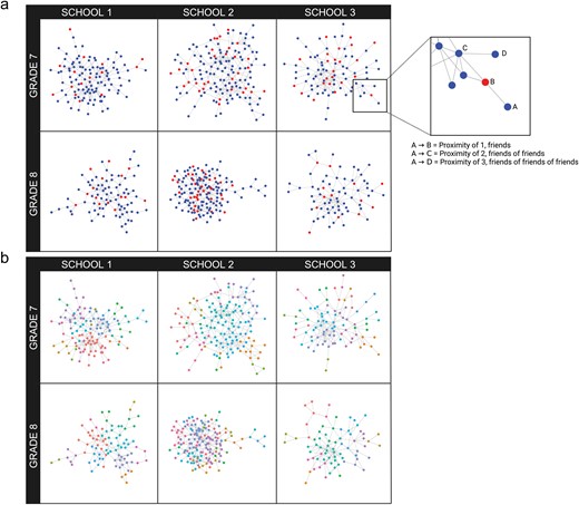
Visual representation of the social networks for the six school-grade groups. Figure created using BioRender.com/v29a02.
Network and sample sizes for each school-grade group.
| School 1 Grade 7 | School 2 Grade 7 | School 3 Grade 7 | School 1 Grade 8 | School 2 Grade 8 | School 3 Grade 8 | |
|---|---|---|---|---|---|---|
| Endorsees | 220 | 311 | 230 | 189 | 268 | 189 |
| Endorsers | 131 | 191 | 115 | 96 | 172 | 92 |
| Network coverage (%) | 59.5 | 61.4 | 50.0 | 50.8 | 64.2 | 48.7 |
| Network size after exclusions | 118 | 145 | 88 | 88 | 150 | 74 |
| Final sample | 10 | 20 | 13 | 14 | 25 | 10 |
Notes: “Endorsees” refers to the total number of students listed on each grade roster and who could have been nominated, whereas “endorsers” refers to the number of participants who offered friendship nominations used to construct the social networks. “Network size after exclusions” refers to the size of the network after isolates and small unconnected groups have been removed. The “final sample” refers to the number of participants from each network who had complete scan data and who were included in the study analyses.
Affective pictures task
During one functional run, participants viewed and rated affective pictures. This task was coded using E-prime 2.0 and completed in the MRI scanner. On each of 120 trials, participants saw a jittered fixation cross (minimum: 539.7 ms, maximum: 4453.3 ms, mean: 2300.101 ms), followed by an image and Likert scale (duration: 2000 ms). Participants were told to rate each image based on how it made them feel. Ratings were made on a 1–5 scale (1 = very negative, 2 = a little negative, 3 = neutral, 4 = a little positive, and 5 = very positive). Images were presented in random order and varied in their affective valence (pleasant, unpleasant, and neutral). Participants were provided instructions and a practice task outside of the scanner before completing the main task. All affective pictures were selected from the normed Open Affective Standardized Image Set (Kurdi et al. 2017). A full list of stimuli and associated norms can be found in Supplementary Table S2.
fMRI data acquisition
Imaging data were acquired on a 3 Tesla Siemens Prisma MRI scanner. During scanning, participants completed both structural and functional scans. All MRI data were preprocessed using “fMRIprep” v1.5.3 (Esteban et al. 2019), and postprocessing was conducted using a custom script described in Dai et al. (2023) and available at https://osf.io/svbpq/. More details can be found in Supplementary Notes 1.
Region of Interest Selection
Analyses were run within five regions of interest: two implicated in the computation of affective valence (vmPFC and temporal pole), two implicated in the representation of affective salience (bilateral amygdala and anterior insula), and the primary visual cortex (control) (Kober et al. 2008, Lindquist et al. 2012, 2016). Region of interest (ROI) masks for bilateral amygdala and bilateral temporal pole were taken from the Harvard Oxford Subcortical and Cortical Atlases using probability thresholds of 50% (Desikan et al. 2006, Frazier et al. 2005, Goldstein et al. 2007, Makris et al. 2006). Bilateral insula masks were taken from the Harvard Oxford atlas using a probability threshold of 50% and trimmed to include only the anterior portion. The ROI mask for vmPFC was constructed using a 10-mm sphere around peak coordinates defined in Roy et al. (2012), and the ROI mask for primary visual cortex was taken from the parcellation defined in Shirer et al. (2012).
Computing dyadic neural similarity using multivoxel similarity
Dyadic neural similarity was computed for each ROI for each valence condition of the affective pictures task for each unique dyad in our data. We first computed a trial by voxel matrix representing activation within a given ROI across all trials of a given valence condition (see Fig. 2, Panels 1 and 2). To compute trial by voxel matrices, we extracted regression coefficients from trial-wise general linear modeling (GLM). These trial-level estimates were obtained using a least-squares analytical framework (Rissman et al. 2004, Abdulrahman and Henson 2016) to control for collinearity in BOLD responses to successive trials (Turner et al. 2010, Mumford et al. 2012). This method estimates a separate GLM for each trial controlling for all other nontarget trials as confounds. Single-trial activity responses to each affective image were then extracted from each ROI for each valence condition for each participant using the Nilearn package (Abraham et al. 2014). From this trial by voxel matrix, we computed a square correlation matrix characterizing the coactivation of voxels within a given ROI across stimuli of a given valence condition (Fig. 2, Panel 3) (Kriegeskorte et al. 2008, Kriegeskorte and Kievit 2013). The upper diagonals of these correlation matrices were then vectorized and used to compute pairwise correlations (i.e. “neural similarity”) (Fig. 2, Panel 4). The final estimates of neural similarity were then Fisher z transformed.
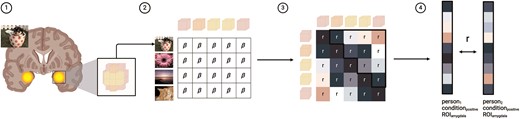
Schematic of methods for computing dyadic neural (multivoxel) similarity. Figure created using BioRender.com/e28r758.
Final models
Main analyses were run using the lmer MultiMember package in R (van Paridon and Bolker 2023), which was designed to expand functionality of the lme4 (Bates et al. 2015) to include multiple membership random effect structures. These packages use the Satterwhite method to estimate degrees of freedom. Multiple membership models (MMMs) are similar to cross-classified effect models but are designed for situations where observations are nested within more than one level of a single random effect (Rasbash and Browne 2008, Goldstein 2011) (Fig. 3). In this instance, we used MMMs to model unique dyads, nested within each of their constituent members using a uniform weighting scheme where all weights were set equal to 1. For similar methods, see Dean et al. (2017). All models controlled for whether dyad members were matched on gender, race, and ethnicity as these demographic variables are established sources of homophily (McPherson et al. 2001). For each set of models within a given ROI, P-values were corrected for multiple comparisons using a Benjamini–Hochberg (BH) correction (Benjamini and Hochberg 1995). Corrections for multiple comparisons were achieved using the “p.adjust” function from the stats package in R (R Core Team 2023). Diagnostics were used to confirm the relative normality and homoscedasticity of model residuals.
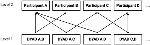
Final model nesting diagram; multiple membership structure. Figure created using BioRender.com/b73s078.
Power
Given that this was a secondary data analysis, sample size was fixed. Furthermore, all students from a given school district were invited to participate in this study placing an upper bound on our sample size. Despite this, a priori power analyses for two-tailed t-tests on single regression coefficients from a linear multiple regression with four predictors were run in g*power (Faul et al. 2007). Analyses revealed that a sample size of 395 would be sufficient for detecting a small effect (f2 = 0.02) at α = 0.05 and 1 − α = 0.80. Because analyses were done using nested data using mixed models, power analyses for multiple regression represent conservative estimates. Consequently, our sample size of 749 dyads should be sufficient.
Data and code availability, transparency, and openness
All code and analyses are available at https://osf.io/svbpq/. This study’s design was not preregistered. However, hypotheses and analyses were preregistered with post hoc adjustments (Supplementary Table S1). Unrestricted sharing of anonymized data was not detailed in this study’s ethical review application nor in consent forms, and therefore data are not uploaded to a public repository. However, data are available by reasonable request pending completion of appropriate data sharing agreements.
Results
Regression models tested two key hypotheses. First, we assessed whether teens’ social network proximity predicted their neural similarity. Second, we assessed whether individuals in the same friend group, as determined by data-driven clustering, demonstrated greater neural similarity compared to individuals in different friend groups. All regressions controlled for whether dyads were matched on gender, race, and ethnicity. Corrections for multiple comparisons were applied. Full regression tables for each region and affective condition can be found in Supplementary Tables S3 and S4.
Predicting neural similarity during affective experience with dyad-level social network proximity
Social proximity was a significant predictor of neural similarity in the vmPFC for pleasant [F(1, 713.74) = 7.68, P = .01, PBH = .02] and neutral [F(1, 735.18) = 5.43, P = .02, PBH = .03] but not unpleasant [F(1, 722.98) = 2.94, P = 0.09, PBH = 0.09] images when controlling for model covariates. Specifically, as adolescents moved further and further apart in their social network, neural similarity in the vmPFC to pleasant and neutral images decreased (Fig. 4a–c). Social network proximity did not significantly predict neural similarity for pleasant, unpleasant, or neutral images in any of the other regions of interest (all PBH values > .24). See supplementary table 3.
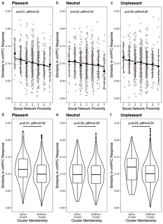
Simple regression plots visualizing the relationship between social network proximity and neural similarity in the vmPFC to pleasant (a), neutral (b), and unpleasant (c) images. Violin plots visualizing the mean difference in neural similarity in the vmPFC to pleasant (d), neutral (e), and unpleasant (f) images for individuals in the same and different friend groups or clusters.
Predicting neural similarity during affective experience based on cluster membership
Complimenting some of our dyad-level analyses, we found that friend group membership (i.e. belonging to the same friend group versus different group) was a significant predictor of neural similarity in the vmPFC for pleasant [F(1, 697.83) = 6.62, P = .01, PBH = .03] and unpleasant [F(1, 694.02) = 4.83, P = 0.03, PBH = 0.04], but not neutral [F(1, 689.67) = 0.75, P = 0.39, PBH = 0.39] images when controlling for model covariates. Specifically, individuals who were in the same friend group (i.e. cluster) demonstrated greater neural similarity on average in the vmPFC for positive and negative images than individuals who were in different friend groups (Fig. 4d–f). Cluster membership did not significantly predict neural similarity for pleasant, unpleasant, or neutral images in any of the other regions of interest (all PBH values > .37) see Supplementary table 4.
Supplemental models
Additional models assessing whether effects were robust when controlling for time elapsed between scan session and in-laboratory sociometric data collection are presented in Supplementary data. These models used sum and product terms to explore the unique and joint effects of time elapsed for each dyad member. Results did not change with the addition of these covariates. Full model results can be found in Supplementary Tables S5 and S6.
Discussion
The tendency for “birds of a feather” to “flock together”, or homophily, is a well-documented feature of social networks (Kandel 1978, McPherson et al. 2001). Recent evidence suggests that homophily may extend to the brain—such that those closer within adult social networks demonstrate more similar patterns of neural responding during rest and while viewing both static and dynamic stimuli (Parkinson et al. 2018, Hyon et al. 2020a, 2020b, Baek et al. 2022). Many of these existing studies focused on neural similarity during movies or narratives that have affective qualities, but did not test neural similarity during affective experiences, per se. This study builds upon prior work by evaluating whether those closer in adolescent social networks have more similar patterns of neural responding during affective experience. Specifically, we evaluated how social proximity (measured as geodesic distance) within adolescents’ school-based social networks predicted neural similarity when viewing pleasant, unpleasant, and neutral stimuli. To our knowledge, there is only one study to date examining the role of neural similarity in adolescent social networks. This study found null effects of friendship on neural similarity during a passive rest condition among girls aged 12–13 years (McNabb et al. 2020). Yet examining spontaneous thought at rest is not ideally suited to revealing whether and how similarity in affective experiences is associated with friendship in adolescents. Using multivoxel similarity analysis of neural responses to affective experiences, we were able to shed light on the neurocognitive mechanisms that may underlie the role of affective similarity in adolescent friendships. We found that adolescents closest to one another in their school network had more similar neural representations of pleasant and neutral, but not unpleasant stimuli (although this effect was marginal) within the vmPFC, but not other regions associated with affective experience or visual processing. Exploratory analyses also revealed that adolescents in the same (versus different) friendship groups (estimated using data-driven clustering) had more similar patterns of neural responding in the vmPFC to both pleasant and unpleasant stimuli. These results contribute to our understanding of how adolescents’ neural representations of salient affective stimuli relate to the nature of their friendships and the structure of their broader social networks.
Role of the vmPFC and affective processing
The present analyses examined predictors of neural similarity within the primary visual cortex, amygdala, insula, temporal pole, and vmPFC. A significant effect of social network proximity on neural similarity in the amygdala or insula may have suggested a role for similarity in affective reactivity or salience detection in homophily. The specificity of our results to the vmPFC thus suggests an alternative interpretation. While the temporal pole and the vmPFC are both higher-order brain regions implicated in affective meaning-making, the vmPFC is implicated in representation of affective valence in particular (Lindquist et al. 2016, Rolls 2019). That is, the vmPFC integrates information from the external environment (sights, sounds, smells, tastes, etc.), the internal body, and prior experiences drawn from long-term memory to make sense of on-going experience, including whether that experience is pleasant or unpleasant (Satpute and Lindquist 2019). Prior studies assessing neural similarity also find effects in higher-order brain regions implicated in domain-general meaning-making (Wilson et al. 2008, Li et al. 2014). Indeed, while neural activity in unimodal regions like primary visual or auditory cortex tends to temporally synch across individuals exposed to the same stimuli, neural activity in the vmPFC is highly idiosyncratic—reflecting individual’s unique histories, interpretations, and goals (Chang et al. 2021). Furthermore, vmPFC is relatively more synchronized when dyads are viewing affective versus nonaffective scenes (Chang et al. 2021), suggesting its relatively unique role in making “affective” meaning. Given that neural similarity can underlie shared mental understandings of experiences (Stephens et al. 2010, Lahnakoski et al. 2014, Nguyen et al. 2019), our data suggest that adolescents who are closer in their social network may be more aligned in their appraisals of affectively evocative stimuli. This interpretation is consistent with the fact that neural similarity in responses to pleasant and unpleasant stimuli was consistently associated with social network properties (proximity and/or cluster membership) across our analyses, whereas similarity to neutral stimuli was only associated with proximity. These findings are also consistent with the importance of emotion in social relationships (e.g. Graham et al. 2008), which is perhaps heightened during adolescence.
Emotion representation and implications in adolescence
Adolescence is a developmental phase marked by an emerging need to make sense of increasingly frequent, intense, and complex affective experiences (Bailen et al. 2019). As neurobiological and social changes reorient adolescents toward their peers (Blakemore and Mills 2014, Nelson et al. 2016), social networks may become increasingly relevant for the socialization of emotion representation, expression, and regulation (Klimes-Dougan et al. 2014; Shipkova et al. forthecoming). This kind of socialization may contribute to increasingly similar emotion concepts among peers (Camacho et al. 2023). Our observed findings—that neural responses to affective stimuli are most similar among friends—may corroborate this notion. Notably, while similarity in neural responses to pleasant stimuli was associated with both friendship proximity and friendship clusters, similarity for unpleasant stimuli was only significantly associated with cluster membership. Given that friendship clusters are salient features of adolescents’ social lives that can influence them beyond the effects of individual friendships (Ellis and Zarbatany 2017), these results may indicate that socialization of unpleasant emotion representation may occur more at the friend group level. Additionally, when interpreting these results, it is important to consider how network structure and related effects may differ by the operationalization of a friendship tie. We use “close friendship” as our operationalization, but it should be noted that networks defined by looser social relationships (such as those that focus on who you communicate with frequently or even if you are familiar with someone or not) may be denser. In these denser networks, the types of results we observed—in which friends had more similar neural representations of emotions—might be concentrated across fewer degrees of separation. Additionally, in future research, the construct of “friendship” could be further explored. For instance, network structure and positionality can differ based on relationships characterized by being “fun” or “exciting” versus those that are characterized by “trust” and “support” (Morelli et al. 2017). These different types of friendships might have especially interesting implications for emotional similarity in adolescents.
Contributions, limitations, and future directions
Despite the many contributions of this work, our findings are not without limitations. For example, there is some debate over whether current methods for fMRI afford the spatial precision to enable intersubject correspondence mapping of voxel-wise activation patterns (Kriegeskorte and Bandettini, 2007). For example, it is likely that fine-scale functional organization within a given brain region is highly individuated across participants (Kriegeskorte and Bandettini, 2007). This possibility implies that our method is likely quite conservative, in that it is identifying intersubject similarities at the voxel level. Future work should also replicate and extend these findings with other multivariate methods for computing intersubject similarity (e.g. see Parkinson et al. 2018, Hyon et al. 2020a, Baek et al. 2022). It is worth noting that any pre-existing issues with spatial precision would be exacerbated in the temporal pole, a region that is particularly vulnerable to susceptibility artifacts resulting in signal dropout and distortion (Devlin et al. 2000, Visser et al. 2010), making it more challenging to find effects in this region.
Another limitation of the present analyses is that we focus on multivoxel brain representations of valence, but not arousal. Stimuli used in this study were designed to allow for comparison between neural reactivity to normatively high-intensity unpleasant stimuli and normatively high-intensity pleasant stimuli. They were not chosen to range in intensity or arousal. This limits our ability to determine whether effects differed for high versus low arousal affect within a valence category or for high versus low intensity affect within a valence category. Answering this question about the specificity with which vmPFC is representing the affective similarity of stimuli would be an interesting future direction. Given the role of the amygdala and insula in encoding affective salience, the lack of variance in stimuli arousal may have contributed to our inability to identify effects in these regions, although caution must be exercised in interpreting null results. Future work should explore whether effects replicate for stimuli representing different quadrants of the affective circumplex. Additionally, our findings are limited by our use of a cross-sectional sample. It is thus not possible to determine whether our effects reflect selection or socialization processes. Adolescents may choose friends with similar affective experiences (i.e. selection). It is also possible that adolescents’ affective experiences change to resemble their friends’ affective experiences over time (i.e. socialization). Since adolescence is characterized by both dynamic friendship networks and the development of more sophisticated emotion concepts (Nook and Somerville 2019, Camacho et al. 2023), it is likely that both processes are at play. Indeed, previous longitudinal studies have identified both selection (Schaefer et al. 2011, Elmer et al. 2017) and socialization (van Workum et al. 2013, Klimes-Dougan et al. 2014, Block and Burnett Heyes 2020) effects on emotional well-being and mood in adolescent and young adult samples. Another limitation of our cross-sectional study is that we exclusively examined early adolescence (ages 11–13 years). Since there is evidence that emotion concept knowledge continues to develop through at least age 18 years (Nook et al. 2017, Nook and Somerville 2019), it would be interesting to examine these effects longitudinally and at different points across the transition to adulthood. Nonetheless, our study builds upon the previous literature assessing neural similarity in social networks by examining generalization in adolescent social networks and during affective experience, in particular. These findings contribute to our understanding of how similar interpretations and experiences of affective stimuli relate to adolescent friendships and social networks more broadly.
Author contributions
Mallory J. Feldman (Conceptualization, Methodology, Software and formal analysis, Data curation, Writing—original draft, Writing—review and editing, Visualization), Jimmy J. Capella (Conceptualization, Methodology, Software and formal analysis, Data curation, Writing—original draft, Writing—review and editing, Visualization), Junqiang Dai (Conceptualization, Methodology, Software and formal analysis, Writing—review and editing), Mitchell J Prinstein (Conceptualization, Methodology, Investigation and resources, Writing—review and editing, Supervision, Project administration, and Funding acquisition), Eva H. Telzer (Conceptualization, Methodology, Investigation and resources, Writing—original draft, Writing—review and editing, Supervision, Project administration, and Funding acquisition), Kevin Lewis (Conceptualization, Methodology, Writing—review and editing), Kristen A. Lindquist (Conceptualization, Methodology, Investigation and resources, Writing—original draft, Writing—review and editing, Supervision, Project administration, and Funding acquisition), Adrienne S. Bonar (Conceptualization, Data curation, Writing—review and editing), and Nathan H. Field (Conceptualization, Data curation, Writing—review and editing).
Supplementary data
Supplementary data is available at SCAN online.
Conflict of interest
To the best of our knowledge, the named authors have no conflict of interest, financial or otherwise.
Funding
This work was supported by grants from the National Science Foundation (SES 1459719 to E.H.T.) and the National Institutes of Health (R01DA039923 to E.H.T., R01DA051127 to E.H.T. and K.A.L., and F31AG081073 to M.J.F.).
References
Author notes
shared first authorship.
