


Abstract
We test the proposition that investors’ ability to cope with financial losses is much better than they expect. In a panel survey of investors from a large bank in the UK, we ask for their subjective ratings of anticipated returns and experienced returns. The time period covered by the panel (2008–10) is one where investors experienced frequent losses and gains in their portfolios. This period offers a unique setting to evaluate investors’ hedonic experiences. We examine how the subjective ratings behave relative to expected portfolio returns and experienced portfolio returns. Loss aversion is strong for anticipated outcomes; investors are twice as sensitive to negative expected returns as to positive expected returns. However, when evaluating experienced returns, the effect diminishes by more than half and is well below commonly found loss aversion coefficients. This suggests that a large part of investors’ financial loss aversion results from an affective forecasting error.
1. Introduction
Loss aversion has been frequently documented in psychology and economics, with the conclusion that losses loom larger than gains and that even “attractive” lotteries from an expected value perspective are often not accepted when they involve potential losses. The magnitude of this effect has been experimentally identified with loss aversion coefficients close to or above two. In finance, loss aversion has been suggested to explain, for instance, the equity premium puzzle and low stock market participation (Benartzi and Thaler, 1995; Ang, Bekaert, and Liu, 2005).
In the evaluation of gains and losses, one has to distinguish between anticipated and experienced outcomes. Most experiments on gambles or lotteries focus on the trade-off between anticipated gains and losses. However, this implies that people are able to perfectly forecast the hedonic impact of gains and losses. In contrast, recent experimental evidence suggests that people’s ability to cope with losses is much better than they predict (Kermer et al., 2006). When actually experienced, losses seem not to hurt as much as people expected.
Using a unique dataset, we test this proposition in the financial domain. In a panel survey of investors from a large bank in the UK, we ask for their subjective ratings of anticipated and experienced returns. Within the time period covered by the panel (2008–10), we observe frequent losses and gains in both the stock market and in investors’ portfolios. This provides the required return distribution to analyze investors’ hedonic experiences. We examine how their subjective ratings of outcomes behave relative to expected and experienced portfolio returns. We calculate loss aversion coefficients for expectations and experiences and define several potential reference points investors might use. Inferences are drawn from the cross-section of investors as the survey design does not allow an estimation of individual loss aversion coefficients.
The results demonstrate that loss aversion is strong for anticipated outcomes. From the regressions of subjective ratings on expected returns, we infer a loss aversion coefficient of about 2.2 using a reference point of zero. This means that investors react twice as much to negative expected returns as to positive expected returns. While for different reference points and model specifications loss aversion coefficients vary slightly, they are almost always close to two and statistically significant.
However, when evaluating experienced returns, the loss aversion coefficient decreases to about 1.2 and is statistically indistinguishable from one (loss neutrality). This holds irrespective of the used reference point or regression model. Investors do not react more strongly to losses than to gains when they are reflecting about their past portfolio performance. The loss aversion they show ex ante seems to be partly or fully an affective forecasting error (i.e., a failure to accurately predict future utility). The result is independent of whether we use a percentage return or monetary profits as the outcome variable.
As a second property of reference-based utility, we also test for diminishing sensitivity with respect to outcomes more distant from the reference point. We indeed find that investors’ reaction is strongest for returns close to the reference point. An improvement in portfolio returns from 2 to 4% has a greater impact on subjective ratings than moving from 12 to 14%. This is true both for expected and experienced returns. Although the sensitivities for expected returns in each interval are greater for losses than gains, this is not the case for return experiences.
Our findings have practical implications for investing behavior. While loss aversion is a legitimate part of people’s preferences, the financial loss aversion illusion we document represents an inconsistency in how a loss is viewed at different points in time. If investors systematically overestimate their personal loss aversion when thinking about financial outcomes, then their investment decisions will differ from what is justified by their actual experiences. In particular, they will invest in less risky assets than would be optimal from an ex post perspective and will avoid potential losses unless they receive a substantial compensation.
To provide evidence on the consequences of loss aversion for investment behavior, we analyze the portfolio risk investors take. We interact gains and losses with portfolio volatility and find that higher loss aversion is associated with less risky portfolios. This suggests that the loss aversion coefficients we measure are meaningful for participants’ investing behavior. We assume that with a greater awareness of their future gain and loss experience, investors would be prepared to take on higher portfolio volatility. An even stronger result on individual level is prevented by the aggregated loss aversion estimates.
We further investigate the nature of financial loss aversion illusion by examining the effects of learning and sophistication. We find that previous losses reduce anticipated loss aversion. Investors seem to learn from the immediate experience of a loss and more accurately predict their responses to future outcomes. However, this learning effect is short-lived. Financial literacy and investment experience are measures of investor sophistication that mitigate financial loss aversion illusion. In extensive robustness analyses, we test for risk aversion as an alternative explanation, examine the exclusion of several types of observations, and analyze the impact of selection effects.
Our work is related to two strands of the literature. We contribute to research in decision theory and psychology on estimating loss aversion (Tversky and Kahneman, 1992; Abdellaoui, Bleichrodt, and Paraschiv, 2007), and apply it to the domain of individual investing. In particular, we test the prediction of a difference between anticipated loss aversion and loss experience (Kermer et al., 2006), which belongs to a broader class of affective forecasting errors (Kahneman and Snell, 1990; Wilson and Gilbert, 2005). Second, we contribute to the large literature on loss aversion in finance (reviewed in Section 2) by showing that loss aversion is present in the portfolio expectations of investors and that it is potentially responsible for the portfolio risk investors take. By revealing the discrepancy between these expectations and the experience of the actual outcomes, we provide new insights on the role and consequences of loss aversion in investing.
2. Theory and Literature
When confronting a bet with equal chances for a gain and a loss, people typically require a gain that is much larger than the loss to accept the bet. Samuelson (1963) reports offering such a bet to colleagues, which was often declined even when the potential gain was $200 compared with a potential loss of $100. This cannot be explained by risk aversion alone as risk premia are generally much lower for gambles completely in the gain domain. Instead, it seems that losses loom larger than gains: in the example, more than twice as large. At the same time, this means that outcomes are viewed from a reference point, which defines gains and losses relative to this reference. The idea that people adapt to a reference level can be found in the psychology literature around the time of Samuelson’s observation (Helson, 1964).
Loss aversion coefficients have typically been empirically estimated using monetary lotteries. Tversky and Kahneman (1992) report a median coefficient of 2.25, while Fishburn and Kochenberger (1979) find a median coefficient of 4.8. Abdellaoui, Bleichrodt, and Paraschiv (2007) calculate median coefficients between 1.53 and 2.52, depending on the estimation method. Abdellaoui, Bleichrodt, and L’Haridon (2008) report coefficients between 2.24 and 3.01 for different prospects. Booij and van de Kuilen (2009) observe loss aversion coefficients between 1.73 and 2.00 depending on the estimation method and whether the lotteries involve high or low stakes. Lower loss aversion coefficients are found in other experiments: 1.43 (Schmidt and Traub, 2002), 1.8 (Pennings and Smidts, 2003), 1.58 (Booij, van Praag, and van de Kuilen, 2010), 1.23 and 1.46 (Zeisberger, Vrecko, and Langer, 2012). Many of these studies also examine individual loss aversion and conclude that the large majority of participants are loss averse.
In these elicitation tasks of loss aversion, the parameters are mostly inferred from participants’ choices between two lotteries or between a lottery and a certainty equivalent. People have to think about a lottery before it is played and have to anticipate how different outcomes would feel. Or more technically, they have to assign an expected utility to each outcome. Possibly, the experience of an actual outcome will differ from expectations ex ante. Loss aversion could result from an affective forecasting error, if people are inaccurate in assessing the hedonic consequences of a risky decision involving gains and losses. In particular, they might fear potential losses to a greater degree than justified. Similar forecasting errors are quite common in evaluating future utility, often due to an overestimation of the impact of an outcome (Wilson and Gilbert, 2005). The two different perspectives have also been labeled “decision utility” and “experienced utility” and they can differ in systematic ways (Kahneman, Wakker, and Sarin, 1997).
Only rarely do experiments on loss aversion take experienced utility into account. As an exception, Kermer et al. (2006) compare predicted changes in happiness to experienced changes in happiness in a between-subject and a within-subject design. They find in both cases that people predict losses will have a greater emotional impact than gains, but do not feel an experienced loss more strongly than a gain. Their ability to come to terms with losses seems to be better than they expected. In contrast, for loss aversion under certainty (the endowment effect), people underestimate their degree of loss aversion before receiving an object (Loewenstein and Adler, 1995). Imas, Sadoff, and Samek (2017) find that participants in a real-effort task correctly predict they will work harder under a contract in which they can lose an endowment. It is hard to tell from their results, whether participants are also correct about the degree of their loss aversion.
We take this laboratory evidence to the field of investment decisions, for which we obtain a unique data set of return evaluations and actual choices by retail investors. We test both predictions by examining whether investors are loss averse with respect to their expected portfolio returns (Hypothesis 1) and whether the higher relative impact of losses declines or even disappears when evaluating experienced portfolio returns (Hypothesis 2). This setting allows us to test numerous additional predictions and alternative explanations. We also extend Kermer et al. (2006) in methodology by suggesting ways to calculate loss aversion coefficients and quantifying the financial loss aversion illusion.
The application to the investment context is motivated by the importance of loss aversion in financial decisions. Most investments involve potential gains and losses, thus loss aversion has received a lot of attention, both theoretically and empirically. Benartzi and Thaler (1995) introduce loss aversion as an explanation for the equity premium puzzle. Combined with frequent portfolio evaluation (myopia), loss aversion renders stock investments unfavorable relative to riskless investments. Due to frequent losses in the short term, investors demand a high premium to invest in stocks. Haigh and List (2005) confirm experimentally the presence of myopic loss aversion for professional traders.
Under the additional assumption of narrow framing, high loss aversion can even prompt people to completely abstain from investing in the stock market (Ang, Bekaert, and Liu, 2005; Barberis, Huang, and Thaler, 2006). This addresses a second financial puzzle, which is low participation in stock markets. Dimmock and Kouwenberg (2010) find that households with higher loss aversion are less likely to participate in equity markets. Their study based on a Dutch household survey is among the few to directly measure loss aversion. The relevance of loss aversion extends to portfolio choice and diversification (Polkovnichenko, 2005; Dimmock and Kouwenberg, 2010). It may also have important consequences for retirement investing saving (Benartzi and Thaler, 1999). Barberis and Huang (2001) suggest that investors are loss averse over changes in the value of individual stocks rather than their portfolios. In simulation results, this type of loss aversion explains a variety of stock market phenomena such as excess volatility and the value premium.
3. Data
We conduct a panel survey of direct brokerage clients at Barclays Stockbrokers, one of the largest brokerage providers in the UK. Participants are self-directed retail investors holding mostly stocks and mutual funds in their portfolios. Most of them have had a portfolio with the brokerage for several years. The survey was designed in collaboration with the Behavioural Finance team at Barclays and covers the period between 2008 and 2010. The survey took place quarterly, which results in a total of nine survey rounds. With the volatile stock markets over that period resulting in frequent losses and gains of different magnitudes, the panel provides a unique opportunity to analyze loss aversion from investors’ perspectives.
In a first step, a sample of clients was selected using a stratified sampling procedure, which excluded clients with less than one trade per year or a portfolio value of <£1,000. Apart from these exclusion criteria, the selection was random and the final sample of 19,251 investors is largely representative of Barclays Stockbrokers’ client base. These investors were invited via email to participate in the online questionnaire. Six hundred and seventeen investors participated in the panel for at least one round and we have a total of 2,135 investor-round observations, which means that respondents on average participated about 3.5 times. For each of the nine rounds, we have a minimum of 130 observations.
This corresponds to a response rate of 3%, which is not much lower than in similar surveys (Dorn and Huberman, 2005; Glaser and Weber, 2007).1 The demographics of investors are shown in Panel A of Table I. The participants are predominantly male, older, and more affluent than the overall population in the UK. In this respect, they closely resemble the investor population in other studies on online brokerage clients. The financial literacy among participants is also reasonably high (on average, 3.5 correct responses out of four questions taken from van Rooij, Lusardi, and Alessie, 2011), which suggests that potential biases we identify are not just due to an insufficient understanding of financial markets.
The two survey questions we mainly focus on are subjective ratings of expected returns and experienced returns:
1. How would you rate the returns you expect from your portfolio held with us in the next three months? Seven-point scale from “extremely bad” to “extremely good.”
2. How would you rate the returns of your portfolio (all investments held with us) over the past three months? Seven-point scale from “extremely bad” to “extremely good.”
The first question asks investors to provide a rating of their expected portfolio returns over the next 3 months. This corresponds to the time interval between two survey rounds. The second question is the mirror image of the first question, asking for a rating of past portfolio returns over the last 3 months. We use the exact same format for both questions, to ensure that participants interpret the scope of the questions in a similar way. In addition, as McGraw et al. (2010) point out, a common scale is important when comparing different evaluations of gains and losses. The ratings are elicited on a good-to-bad scale and provide a subjective evaluation of the expected and experienced returns rather than a numerical estimate (which we also ask, see below). We interpret the rating as a proxy for the utility an investor associates with the expected or experienced returns, respectively. In Equations (1) and (2), the ratings represent u(x), with for the first question and for the second question.
Similarly, Merkle, Egan, and Davies (2015) use the second question to determine investor happiness, while Kermer et al. (2006) ask “how happy” participants feel (or predict to feel) after particular outcomes. It is common in psychology to assess the hedonic quality of an item or experience using a simple good to bad scale (Osgood, Suci, and Tannenbaum, 1957; Kahneman, Diener, and Schwarz, 1999). In economic terms, the ratings express anticipated utility with a return in asking how “good” a certain outcome is expected to be. The link between such subjective evaluations and utility is advocated in economic happiness research (Frey and Stutzer, 2003; Oswald and Wu, 2010). However, some respondents may have interpreted this question as asking for the expected level of returns rather than their feelings regarding the level of returns. To exclude this possibility, we run a validation study with UK participants in which we include a direct question for happiness. We find a correlation between the alternative question formats of 0.76 (and even 0.87 for a subsample of investors; for details see Supplementary Appendix A). We conclude that investors understand the question for ratings of past or expected returns similarly to a question for experienced or expected happiness.
Panel B of Table I shows descriptive statistics for the responses to these questions. The average expected portfolio return rating of 4.2 is slightly above the middle point of the scale, while the average experienced return rating is 3.6. The poor performance of the stock market during the survey period certainly contributed to the low experience ratings. Quite reasonably, experienced return ratings are more dispersed than the expected return ratings. When thinking ahead, it would be bold to expect extremely positive or extremely negative outcomes, while ex post (in particular between 2008 and 2010) participants often experience such extreme outcomes.
It is central to our approach to link the subjective ratings to numerical portfolio return data. For the anticipated ratings, we use the numerical expected portfolio returns, and for the experienced ratings, the numerical perceived past portfolio returns, which correspond to x in Equations (1) and (2). We also calculate actual past portfolio returns from investors’ portfolios, but—as Merkle, Egan, and Davies (2015) show—perceived values have a higher relevance for participants. Expected portfolio return and perceived past portfolio return are elicited from participants in the following way:
3. We would like you to make three estimates of the return of your portfolio held with us by the end of the next three months. Your best estimate should be your best guess. Your high estimate should very rarely be lower than the actual outcome of your portfolio (about once in 20 occasions). Your low estimate should very rarely be higher than the actual outcome of your portfolio (about once in 20 occasions).
Please enter your response as a percent change, i.e. a rise as X%, or a fall as -X%.
4. What do you think your return (percentage change) with us over past three months was?
Please enter your response as a percent change, i.e. a rise as X%, or a fall as -X%.
From Question 3, we use the best estimate as the value for expected portfolio return. Panel B of Table I shows quarterly portfolio return expectations are quite high; the median estimate is 5%. They vary widely, including also negative return expectations (n = 173). One might question whether it is rational to expect negative returns for a stock portfolio. However, 41% of participants hold a negative expectation for either their portfolio or the market at least once during the survey period. This fraction rises to 60% when we consider only those who participate at least five times. Thus negative expectations are quite common and not concentrated among a few participants. At the same time, these expectations may not seem totally unreasonable given the frequently observed negative realized returns over that period.
Negative return expectation are not special to this survey, but occur in many of the investor surveys analyzed by Greenwood and Shleifer (2014), and also in forecasts by financial professionals (Hoffmann, Iliewa, and Jaroszek, 2017). There are many reasons why investors hold onto a portfolio for which they expect negative returns. Taxes or transaction costs are among the more reasonable considerations, but inertia might also play a role. In addition, investors might not be overly certain about their expectations or expect a reversal in the longer run. Attempting to time the market is risky and the investor may end up regretting doing so.
The standard deviations in Table I show that expectations are more concentrated than realized returns. We do not observe asymmetries for the gain and loss domains that could affect return ratings. As the table reveals, realized portfolio returns are on average negative for participants (−1.9% perceived and −5.1% actual).2 While participants clearly overestimate their past returns, the correlation between perceived and actual returns is nevertheless high (0.62).
For a reference-dependent model, it is important to define an appropriate reference point. The most obvious reference point is the status quo (r = 0), which means that negative portfolio returns imply a loss and positive returns a gain. Other possible reference points include the risk-free interest rate, inflation, or stock market returns. A loss would then be defined as the underperformance of the portfolio over the last quarter compared with one of these benchmarks. In contrast to the fixed reference point at 0, these alternative reference points are time varying, with the largest variation for stock market returns.
Table I shows descriptive statistics for these benchmarks on a quarterly basis over the sample period. For ease of comparison, the number of observations is adjusted to participation in the individual survey rounds. Inflation as reported by the UK Office for National Statistics was 0.8% on average, which corresponds to an average annual inflation of 3.2%. Short-term interest rates, represented by the 3-month London interbank offered rate, were on average 0.6% on a quarterly basis. Stock market returns were −2.6%, which is in line with investors’ negative realized portfolio returns. Again, we also consider perceived stock market returns, which were elicited analogously to question 4. Perceived market returns were on average −0.8%.
Additionally, market return expectations are a natural reference level for portfolio return expectations. They are elicited in the same way as portfolio return expectations (see Question 3). The results show that market return expectations are considerably lower than portfolio return expectations, which means that investors on average expect to outperform the market. With the expected market return as a reference point, this outperformance would be considered an anticipated gain and underperformance an anticipated loss.
A final set of reference points relies on investors’ individual benchmarks. In each round of the survey, participants are asked what benchmark they currently use, represented as a combination of interest rates and stock market returns.3 Two reference points are constructed: one backward-looking based on realized stock market returns and interest rates of the last quarter, and the other forward-looking based on expected market returns and interest rates for the next quarter. While the averages for these benchmarks lie between the stock market returns and interest rates, they capture more closely the individual reference points of the participants.
4. Results
4.1 Anticipated Loss Aversion
Higher returns feel better subjectively and they provide higher utility to investors. It is therefore not surprising that there is a positive relationship between the expected portfolio returns and the subjective ratings of these returns (correlation 0.40). Figure 1 displays the average subjective rating for each value of expected returns. The dots in the graph mostly represent multiple observations, as the specific values of the expected portfolio returns occur many times in the panel. To represent the subjective ratings by their averages allows for an easier interpretation.
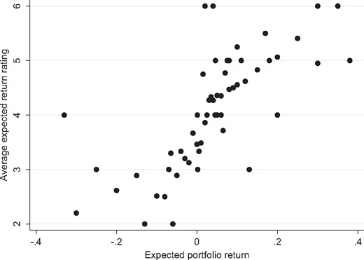
Portfolio return expectations and subjective ratings. Numerical expected portfolio returns and the associated average subjective rating of these returns. Most dots represent multiple observations.
Negative expected returns are mostly rated below four, which is the middle point of the rating scale, while positive returns are mostly rated above four. The point where expected returns cross the neutral rating appears to be somewhere between 0 and 5%. With respect to the functional form, it is difficult to derive definite conclusions from the figure alone, but it seems that the slope is steeper for the lower range of expected returns and flatter for the higher range of returns, which is consistent with loss aversion. There is even an identifiable tendency for a concave relationship for positive expected returns, as well as a convex relationship for losses.
To substantiate these first impressions, we begin with a piecewise linear regression of the expected return ratings on the numerical return expectations. This corresponds to Equation (2) in which the loss aversion coefficient λ represents the ratio between the slopes below and above the reference point. We initially use zero as the reference point, but also report results for other potential reference points. Loss aversion is estimated on an aggregate basis, as there is only one observation of expected return ratings for each individual at each point in time. This represents a limitation as estimates of loss aversion may be contaminated by cross-sectional heterogeneity in investors’ preferences, or changes in individuals’ preferences over time.
We first estimate a pooled ordinary least squares (OLS) model with robust standard errors for the anticipated subjective ratings of returns with expected portfolio returns as a sole explanatory variable. The resulting coefficient in Column (1) of Table II is positive and strongly significant. To separate the effect for the gain and loss domains, we construct a dummy variable for expected gains and losses, respectively. By interacting each dummy with the expected portfolio returns, we estimate two independent coefficients conditional on whether a loss or a gain is expected. For the same regression model as before, the coefficient is 7.5 for losses and 3.5 for gains (see Column (2)). The slope for losses is much steeper than for gains, indicating a strong loss aversion.
Descriptive statistics
The table shows descriptive statistics (number of observations, mean, median, standard deviation, 5% percentile, and 95% percentile) for the main survey variables. Panel A shows the demographics of participants. Number of observations varies due to non-responses. Gender is a dummy variable taking a value of one for male participants. Age is reported in years. Couple is a dummy variable taking the value of one for married or cohabiting participants. Wealth and income are categorical variables, for category values see the Appendix A. Financial literacy is the number of correct responses using four questions (two basic, two advanced) from van Rooij, Lusardi, and Alessie (2011). Experience is self-reported investing experience in years.
Panel B shows participants’ subjective ratings for expected portfolio returns and experienced portfolio returns. It displays numerical estimates of the expected portfolio returns and perceived past portfolio returns. For details on the used survey questions, see Appendix A. Past actual portfolio returns are calculated from investors’ portfolios. For the UK stock market, the actual and perceived performance of the FTSE all-share index are displayed, as well as expectations for 3 months returns of the same index. Interest rates are the 3-month LIBOR, inflation is based on the UK consumer price index. Individual benchmarks are calculated as described in the Appendix A.
aObservations are conditional on survey round participation.
bObservations are constant in the cross-section.
| Panel A | n | Mean | Median | Std.Dev. | 5p | 95p |
|---|---|---|---|---|---|---|
| Gender (male=1) | 617 | 0.93 | 1 | 0.25 | 0 | 1 |
| Age (in years) | 613 | 51.4 | 53 | 12.9 | 29 | 72 |
| Couple | 616 | 0.74 | 1 | 0.44 | 0 | 1 |
| Wealth (nine categories) | 502 | 4.80 | 5 | 2.39 | 2 | 9 |
| Income (eight categories) | 494 | 3.88 | 4 | 1.80 | 1 | 8 |
| Financial literacy (four questions) | 614 | 3.49 | 4 | 0.68 | 2 | 4 |
| Experience (in years) | 197 | 19.5 | 20 | 10.3 | 6 | 38 |
| Panel B | ||||||
| Rating of expected return | 2,107 | 4.18 | 4 | 1.16 | 2 | 6 |
| Rating of experienced return | 2,115 | 3.61 | 4 | 1.73 | 1 | 7 |
| Portfolio return expectation | 2,108 | 0.061 | 0.050 | 0.112 | −0.050 | 0.200 |
| Past portfolio return (perceived) | 2,115 | −0.019 | 0.000 | 0.193 | −0.300 | 0.250 |
| Past portfolio return (actual) | 2,081a | −0.049 | −0.030 | 0.261 | −0.521 | 0.283 |
| Market return expectation | 2,121 | 0.031 | 0.030 | 0.103 | −0.100 | 0.150 |
| Past market return (perceived) | 2,108 | −0.008 | 0.000 | 0.178 | −0.250 | 0.220 |
| Past market return (actual) | 2,135a,b | −0.026 | −0.081 | 0.128 | −0.196 | 0.205 |
| Interest rate | 2,135a,b | 0.006 | 0.004 | 0.005 | 0.001 | 0.014 |
| Inflation | 2,135a,b | 0.008 | 0.008 | 0.003 | 0.003 | 0.013 |
| Individual benchmark (past) | 2,135 | −0.007 | 0.002 | 0.079 | −0.126 | 0.114 |
| Individual benchmark (expectations) | 2,135 | 0.023 | 0.017 | 0.089 | −0.065 | 0.100 |
The loss aversion coefficient λ can be calculated by dividing the coefficient for losses by the coefficient for gains (, see Equation (2)). As a result, we obtain a λ of 2.1, which is in the upper range of the values typically found in experiments based on lotteries. In experiments, the decisions are either hypothetical or the participants receive an endowment upfront to wager. They normally cannot lose their own money, which might attenuate loss aversion. As a caveat, in our setting only the most pessimistic investors hold negative return expectations. If those investors were also more loss averse, this might inflate the estimate. To address issues with the aggregate estimate, we explore in a validation study how investors evaluate several potential returns that are provided to them (see Supplementary Appendix A). While this approach has methodological challenges, we also find evidence for loss aversion on individual investor level.
To make use of the panel structure of the data, we estimate panel regressions shown in the remaining columns of Table II. The results remain unchanged in a generalized least squares (GLS) regression with random effects and standard errors clustered by participants (Column (3)), and they are robust to the inclusion of survey round fixed effects (Column (4)). Finally, we run fixed effects regressions to control for all time-invariant individual effects (Columns (5)–(7)). While the size of the coefficients changes, their ratio expressed in loss aversion λ is unaffected. We also control for investors’ risk tolerance, their subjective portfolio risk perception, portfolio volatility, portfolio value, and turnover of investors, as these might influence the subjective ratings of returns. The control variables are defined in Appendix A. We find that only risk tolerance has a marginally positive significant effect on the subjective ratings, meaning that risk-tolerant investors rate a given return better.
Loss aversion coefficients are significantly larger than one in all regressions with mostly p <0.01. To avoid nonlinearities, test statistics are computed using a Wald test for equality of the coefficients in the loss and gain domains, which is equivalent to λ = 1. Standard errors for the nonlinear ratio are relatively large, but still the resulting 95% confidence intervals do not include one with one exception. The economic magnitude of the effect is such that for an additional 5% in expected portfolio return in the gain domain, the subjective rating rises by about 0.15. But in the loss domain, the identical 5% results in a change of 0.3. This illustrates that investors are more sensitive to losses.
We now turn to other potential reference points for which we repeat the same regression specifications. Table III only reports the loss aversion coefficients from these regressions. A first alternative is that investors evaluate expected portfolio returns relative to the risk-free interest rate that can be earned over the same horizon. The current interest rate for a 3-month horizon thus is the reference point for the first set of loss aversion coefficients. The results are very close to those for a reference point at 0, as quarterly interest rates are mostly below 1%. The same holds for inflation as a reference point, for which we use the inflation rate in the 3 months after each survey as a proxy for inflation expectations (results using current inflation are very similar).
Anticipated loss aversion
The table shows results for regressions of subjective ratings of expected portfolio returns on numerical expected portfolio return and controls. The results in Columns (1) and (2) are estimated by pooled OLS, the remaining columns contain results of panel regressions with random effects [Columns (3) and (4)] or fixed effects [Columns (5)–(7)]. Expected portfolio return is split for gains and losses with 0 as a reference point. Risk tolerance and subjective portfolio risk are self-reported, survey-based measures as defined in the Appendix A. Portfolio volatility is the 1-year historical volatility of investors’ portfolios at the time of each survey round. Log portfolio value is the natural logarithm of the value of the investors’ portfolios at the bank in pounds. Log turnover is the natural logarithm of trading volume divided by the sum of portfolio value at the beginning and end of a survey round. Time-fixed effects are included in form of round dummies for each round of the survey. Standard errors are robust and for panel models clustered by participant. Coefficients are significant at *p ˂ 0.10, **p ˂ 0.05, ***p ˂ 0.01; t-values are shown in parentheses. The loss aversion coefficient is the ratio between the coefficients for expected portfolio losses and gains (standard errors in parentheses). The Wald test tests for equality of these coefficients (λ = 1). Confidence interval is the 95% confidence interval for the ratio of coefficients (λ).
| Subjective rating of expected return | |||||||
|---|---|---|---|---|---|---|---|
| Pooled OLS | GLS with RE | GLS with FE | |||||
| (1) | (2) | (3) | (4) | (5) | (6) | (7) | |
| Expected portfolio return | 4.152 | ||||||
| (11.40)*** | |||||||
| Expected portfolio return | 7.463 | 6.446 | 5.927 | 6.249 | 5.560 | 5.898 | |
| (if < 0) | (8.69)*** | (7.28)*** | (6.96)*** | (5.81)*** | (5.51)*** | (4.54)*** | |
| Expected portfolio return | 3.538 | 3.051 | 2.917 | 2.683 | 2.543 | 2.603 | |
| (if > 0) | (9.25)*** | (7.75)*** | (7.68)*** | (5.86)*** | (5.77)*** | (5.33)*** | |
| Risk tolerance | 0.041 | ||||||
| (1.78)* | |||||||
| Subj. portfolio risk | −0.057 | ||||||
| (−1.57) | |||||||
| Portfolio volatility | 0.198 | ||||||
| (0.70) | |||||||
| Log portfolio value | 0.035 | ||||||
| (1.44) | |||||||
| Log portfolio turnover | 0.094 | ||||||
| (1.21) | |||||||
| Constant | 3.925 | 3.994 | 3.935 | 3.699 | 4.044 | 3.792 | 3.432 |
| (135.91)*** | (122.81)*** | (95.68)*** | (67.80)*** | (118.20)*** | (67.38)*** | (10.07)*** | |
| R2 | 0.159 | 0.171 | 0.171 | 0.215 | 0.171 | 0.212 | 0.227 |
| Observations | 2107 | 2107 | 2107 | 2107 | 2107 | 2107 | 1866 |
| Time-fixed effects | No | No | No | Yes | No | Yes | Yes |
| Individual-fixed effects | No | No | No | No | Yes | Yes | Yes |
| Loss aversion coefficient λ | 2.11 | 2.11 | 2.03 | 2.33 | 2.19 | 2.27 | |
| (0.36) | (0.42) | (0.41) | (0.60) | (0.58) | (0.71) | ||
| P-value Wald test (λ = 1) | <0.001 | <0.001 | 0.002 | 0.004 | 0.009 | 0.025 | |
| Confidence interval λ | 1.40–2.82 | 1.28–2.95 | 1.22–2.84 | 1.14–3.52 | 1.05–3.32 | 0.87–3.66 | |
When market expectations are used as a reference point, the results change. As market expectations are on average about 3%, the reference point shifts to the right. As a consequence, a greater fraction of expected portfolio returns are in the loss domain (24%). Second, the reference point is now personalized, as the market return expectation of each participant is used. This is the reason why the fixed effects regressions now make a difference. We find significant loss aversion coefficients around 1.8 in these specifications, while the results for the other models are between 1.3 and 1.4 and not significantly different from one (see Table (III)). Finally, we take into account the benchmark participants report they use. For these individual benchmarks, we again find significant loss aversion for all regression models. These results provide support for the first hypothesis that loss aversion is present in the return expectations of investors. The magnitude of loss aversion varies for different reference points and model specifications, but is almost always around 2.
4.2 Loss Experience
Anticipated loss aversion has been a primary concern of previous research, as it is relevant for evaluating possible courses of action, such as choosing a lottery or making an investment. An open question is whether investors also experience a higher loss sensitivity from investment outcomes. According to our estimates, losses are expected to be twice as painful as gains of equal size are pleasurable. The survey question for a subjective rating of past portfolio returns corresponds to this hedonic evaluation (u(x)). Past returns in numerical terms are the associated outcomes (x).
The correlation between perceived past portfolio returns and the rating of these returns is 0.67, which is higher than it was for the respective expectations. The linkage between the return levels and their subjective evaluation is very close. Figure 2 shows this almost monotonous relationship, which appears to be more linear than in the case for return expectations. There is no kink easily identifiable in the figure. The correlation of the subjective ratings with the actual past returns calculated from investors’ portfolios is somewhat lower (0.53), which confirms that for the subjective experience of investors, their own estimates of returns are more important than the realized values.
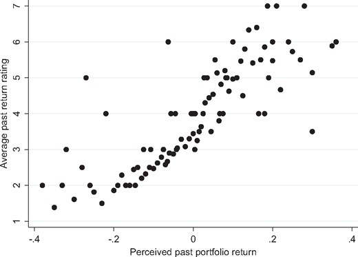
Past portfolio returns and subjective ratings. Numerical perceived past portfolio returns and the associated average subjective rating of these returns. Most dots represent multiple observations.
It is important that we run the same regressions as before to exclude the possibility that some changes in the regression specification are responsible for changes in the results. The parallel approach also satisfies the discussed condition of McGraw et al (2010). Therefore, we start again with a pooled OLS model and a reference point of 0, represented in Columns (1) and (2) of Table IV. The results show that perceived past portfolio returns have a positive impact on the subjective ratings with a coefficient of about six (Column (1)). In economic terms, 5% points in return change the rating by 0.3. The effect is only slightly larger in the loss domain than in the gain domain (Column (2)). We calculate a loss aversion coefficient λ of 1.28.
Anticipated loss aversion for alternative reference points
The table shows loss aversion coefficients for different reference points. Regressions were estimated using the specifications of Table II. λ (interest rate) takes the current 3-month interest rate as a reference point, λ (inflation) the rate of inflation 3-month ahead, λ (market expectations) the market return expectation of participants, and λ (individual benchmark) the individual benchmark of participants. The p-values of a Wald test testing for λ = 1 are reported in parentheses.
| Based on regression model | ||||||
|---|---|---|---|---|---|---|
| (2) | (3) | (4) | (5) | (6) | (7) | |
| λ (interest rate) | 2.09 | 2.09 | 2.02 | 2.29 | 2.16 | 2.24 |
| (<0.001) | (<0.001) | (0.002) | (0.004) | (0.009) | (0.026) | |
| λ (inflation) | 2.11 | 2.11 | 2.03 | 2.32 | 2.18 | 2.27 |
| (<0.001) | (<0.001) | (0.002) | (0.004) | (0.009) | (0.025) | |
| λ (market expectations) | 1.30 | 1.42 | 1.32 | 1.89 | 1.79 | 1.74 |
| (0.238) | (0.135) | (0.253) | (0.009) | (0.027) | (0.035) | |
| λ (individual benchmark) | 1.60 | 1.71 | 1.62 | 2.37 | 2.23 | 2.31 |
| (0.034) | (0.013) | (0.030) | (<0.001) | (<0.001) | (0.001) | |
In a panel model with random effects (Columns (3) and (4)), this result remains unchanged. The coefficients slightly drop when time fixed effects are included in the regression, as they control for the overall stock market performance over time. While expectations may remain relatively stable over different market environments, in retrospect, the survey round effect is more important as it strongly influences individual portfolio returns and return ratings. However, the loss aversion coefficient remains unaffected by this. For the individual fixed effects regressions (Columns (5)–(7)), we find loss aversion coefficients even closer to one depending on the controls. All confidence intervals include the value of one. We again perform a Wald test to examine whether losses have a greater impact on subjective ratings than gains (i.e., whether λ is significantly different from one). Only for one out of six cases do we find significance at the 10% level. Even if some tendency of higher loss sensitivity remains, it is reduced to about 1.2, while the corresponding regressions for expectations yielded loss aversion coefficients around 2.
Considering the regression coefficients for gains and losses in Tables II and IV, it seems that the change in the loss aversion coefficient λ is mainly due to a change in investors’ sensitivity to gains. However, a direct comparison of the coefficients between regressions with different dependent variables is problematic. In Supplementary Appendix B, we normalize the ratings with respect to their means and standard deviations and re-estimate the regressions. The results reveal that a change in the loss sensitivity is mainly responsible for the change in λ.
It is possible that investors use a different reference point when analyzing realized returns. Merkle, Egan, and Davies (2015) show that relative returns are important for investor happiness in the sense that investors compare themselves to the market return. Table V shows the estimated loss aversion coefficients for alternative reference points. Interest rates or inflation make no difference when they are employed as reference points, as they are close to each other and close to 0 over a 3-month horizon. More interesting are the results for past perceived market return and the individual benchmarks as the coefficients are even smaller than those estimated before. They are all in the direct vicinity of one.
Loss experience
The table shows results for regressions of subjective ratings of past portfolio return on numerical perceived past portfolio return and controls. The results in Columns (1) and (2) are estimated by pooled OLS, the remaining columns contain results of panel regressions with random effects [Columns (3) and (4)] or fixed effects [Columns (5)–(7)]. Past portfolio returns are split for gains and losses with 0 as a reference point. Risk tolerance and subjective portfolio risk are self-reported, survey-based measure as defined in the Appendix A. Portfolio volatility is the 1-year historical volatility of investors’ portfolios at the time of each survey round. Log portfolio value is the natural logarithm of the value of the investors’ portfolios at the bank in pounds. Log turnover is the natural logarithm of trading volume divided by the sum of portfolio value at the beginning and end of a survey round. Time-fixed effects are included in form of round dummies for each round of the survey. Standard errors are robust and for panel models clustered by participant. Coefficients are significant at *p ˂ 0.10, **p ˂ 0.05, ***p ˂ 0.01; t-values are shown in parentheses. The loss aversion coefficient is the ratio between the coefficients for past portfolio losses and gains (standard errors in parentheses). The Wald test tests for equality of these coefficients (λ = 1). Confidence interval is the 95% confidence interval for the ratio of coefficients (λ).
| Subjective rating of past return | |||||||
|---|---|---|---|---|---|---|---|
| Pooled OLS | GLS with RE | GLS with FE | |||||
| (1) | (2) | (3) | (4) | (5) | (6) | (7) | |
| Past portfolio return | 5.984 | ||||||
| (perc.) | (22.00)*** | ||||||
| Past portfolio return (perc.) | 6.662 | 6.519 | 4.951 | 6.844 | 4.848 | 4.932 | |
| (if < 0) | (20.38)*** | (18.11)*** | (14.85)*** | (16.21)*** | (10.59)*** | (9.70)*** | |
| Past portfolio return (perc.) | 5.200 | 5.394 | 3.875 | 5.674 | 4.212 | 4.618 | |
| (if > 0) | (8.34)*** | (8.22)*** | (6.43)*** | (8.40)*** | (6.60)*** | (6.08)*** | |
| Risk tolerance | −0.031 | ||||||
| (−1.09) | |||||||
| Subj. portfolio risk | −0.051 | ||||||
| (−1.32) | |||||||
| Portfolio volatility | −0.400 | ||||||
| (−0.73) | |||||||
| Log portfolio value | 0.053 | ||||||
| (1.58) | |||||||
| Log portfolio turnover | 0.078 | ||||||
| (0.47) | |||||||
| Constant | 3.723 | 3.820 | 3.753 | 3.281 | 3.807 | 3.315 | 3.156 |
| (125.04)*** | (72.94)*** | (68.07)*** | (53.11)*** | (65.10)*** | (44.83)*** | (7.59)*** | |
| R2 | 0.449 | 0.452 | 0.452 | 0.517 | 0.452 | 0.515 | 0.529 |
| Observations | 2115 | 2115 | 2115 | 2115 | 2115 | 2115 | 1864 |
| Time-fixed effects | No | No | No | Yes | No | Yes | Yes |
| Individual-fixed effects | No | No | No | No | Yes | Yes | Yes |
| Loss aversion coefficient λ | 1.28 (0.19) | 1.21 (0.18) | 1.28 (0.22) | 1.21 (0.18) | 1.15 (0.21) | 1.07 (0.21) | |
| p-value Wald test (λ = 1) | 0.079 | 0.186 | 0.130 | 0.197 | 0.434 | 0.732 | |
| Confidence interval λ | 0.90–1.66 | 0.85–1.56 | 0.84–1.71 | 0.85–1.56 | 0.73–1.57 | 0.66–1.48 | |
For experienced returns, we consider an additional reference point based on investors’ previous expectations. Falling short of their own portfolio return expectations might be disappointing, which is why they might define gains and losses relative to their expectations. Loss aversion coefficients for this reference point are also close to one. For all results in Table V, the hypothesis that λ = 1 cannot be rejected. We replicate the analysis in the validation study and find no difference between using happiness ratings or return ratings. In the validation sample, the estimated loss aversion coefficients are elevated for anticipated losses () as well as experienced losses (). The gap between the two remains and is slightly larger in magnitude than in the survey data (for details see Supplementary Appendix A).
We conclude that loss aversion in return expectations has no equivalent in return experiences, which confirms our second hypothesis. Survey participants seem to be subject to an affective forecasting error. They appear to believe that negative returns will be painful, but once they learn the actual outcomes, they are not more sensitive to losses than gains. Investors are able to cope with their losses much better than they expected. This also holds true when we repeat the analysis with actual returns instead of perceived returns or monetary outcomes instead of percentage values (see Supplementary Appendices C and D). In the analysis of actual returns, we find no pronounced differences between more recent and more distant outcomes. Coming to terms with losses thus does not appear to be merely an effect of time.
4.3. Comparison of Reference Points
A question remains as to which benchmark is the “true” reference point. Most likely, some investors will use zero, others may use their market expectations, and still others the benchmark they report in the survey question. Since our regression models estimate slopes for the investor population as a whole, it is impossible to determine individual reference points. However, measures on the goodness of fit of these models can provide some indication as to which model is on aggregate most appropriate. We now compare the adjusted R2, the model’s F-statistic, the Akaike information criterion (AIC), and the Bayesian information criterion (BIC) for the different reference points. We use regression model (7) as shown in Tables II and IV as it represents the full model with all controls, but results are robust to the other regression specifications.
Table VI shows the results for the different goodness-of-fit measures. A higher R2 or F-statistic indicates better fit, while for the information criteria (AIC and BIC), lower values represent better fit. The measures favor the reference point at zero for both the anticipated and the experienced outcomes. The inflation and interest rate reference points rank close behind as these reference points are close to zero. Market expectations, portfolio expectations, and market realizations do far worse in terms of goodness of fit. While there are no significance tests on information criteria, conventional rules suggest that a difference of more than 10 signals strong inferiority in terms of fit. The individual benchmarks produce high F-statistics, but fare worse on the other measures.
Loss experience for alternative reference points
The table shows loss aversion coefficients for different reference points. Regressions were estimated using the specifications of Table IV. λ (interest rate) takes the lagged 3-month interest rate as a reference point, λ (inflation) the rate of inflation, λ (market past returns) the past market returns as perceived by participants, λ (individual benchmark) the individual benchmark of participants, and λ (portfolio expectations) the expected portfolio return of the previous survey round. The p-values of a Wald test testing for λ = 1 are reported in parentheses.
| Based on regression model | ||||||
|---|---|---|---|---|---|---|
| (2) | (3) | (4) | (5) | (6) | (7) | |
| λ (interest rate) | 1.28 | 1.21 | 1.28 | 1.21 | 1.15 | 1.07 |
| (0.079) | (0.187) | (0.129) | (0.199) | (0.434) | (0.731) | |
| λ (inflation) | 1.28 | 1.21 | 1.28 | 1.21 | 1.15 | 1.07 |
| (0.079) | (0.187) | (0.129) | (0.198) | (0.433) | (0.731) | |
| λ (market past return) | 1.13 | 1.10 | 1.03 | 1.05 | 0.88 | 0.85 |
| (0.257) | (0.361) | (0.825) | (0.658) | (0.378) | (0.288) | |
| λ (individual benchmark) | 1.11 | 1.07 | 1.04 | 1.06 | 0.92 | 0.95 |
| (0.399) | (0.605) | (0.798) | (0.629) | (0.587) | (0.741) | |
| λ (portfolio expectations) | 0.93 | 0.93 | 0.94 | 1.03 | 0.97 | 0.99 |
| (0.589) | (0.620) | (0.677) | (0.814) | (0.847) | (0.954) | |
Overall, a reference point at zero explains the data best on aggregate. The additional analyses and robustness tests therefore concentrate on this model, but the results in general hold for the other reference points as well. It is interesting that a simple reference point at zero even outperforms the individual benchmarks submitted by participants. It is possible that they report the use of more sophisticated benchmarks, but when it comes to evaluating outcomes fall back on absolute gains and losses.
4.4. Diminishing Sensitivity
Diminishing sensitivity is a property of the prospect theory value function and of other reference-based utility functions. This means that the impact of a change in an outcome decreases with its distance from the reference point (Tversky and Kahneman, 1992). The condition is met, if the utility function is concave in the domain of gains and convex in the domain of losses. In Equation (1), this is the case if parameters α and β are less than one. Empirical estimates for these parameters often vary between 0.5 and 1 (Tversky and Kahneman, 1992; Abdellaoui, Bleichrodt, and Paraschiv, 2007).
It would be desirable to directly estimate the parameters of Equation (1). However, the dependent and independent variables are measured on completely different scales. Thus, one side of the equation would need some arbitrary adjustments. Instead, we continue the piecewise linear approach and split the loss and gain domains into two regions: one close to the reference point and another that is more distant. To provide for a relatively even split of observations, we define returns of up to 5% around the reference point as close. The results are robust to other choices.
Table VII shows the results for this piecewise linear approach, both for expected portfolio returns and experienced portfolio returns. We only report the individual fixed effects models; the results hold for the other specifications as well. For expected returns, sensitivity is largest for small losses with a coefficient of about 20. A change in expected portfolio return of one percentage point here has an effect of 0.2 on the rating of that return. Moving from –5% to 0 thus improves the rating by a whole point. For larger losses, the effect is less strong with a coefficient around 5. A portfolio return of −10% instead of −15% only improves the rating by 0.25.
Goodness of fit for different reference points
The table shows goodness-of-fit measures for models based on different reference points. R2 is the model’s adjusted R2, F-stat, the F-statistic; AIC, the Aikake information criterion; BIC, the Bayesian information criterion. Panel A displays results for anticipated outcomes and Panel B for experienced outcomes.
| Panel A: Anticipated outcomes | ||||
|---|---|---|---|---|
| Reference point | R2 | F-stat | AIC | BIC |
| Zero | 0.187 | 11.74 | 4,086.65 | 4,169.62 |
| (Rank) | (1) | (3) | (1) | (1) |
| Interest rate | 0.187 | 11.75 | 4,087.31 | 4,170.28 |
| (Rank) | (1) | (2) | (3) | (3) |
| Inflation | 0.187 | 11.74 | 4,086.68 | 4,169.65 |
| (Rank) | (1) | (3) | (2) | (2) |
| Market expectations | 0.149 | 11.31 | 4173.71 | 4,256.69 |
| (Rank) | (5) | (5) | (5) | (5) |
| Individual benchmark | 0.186 | 12.02 | 4,090.91 | 4,173.88 |
| (Rank) | (4) | (1) | (4) | (4) |
| Panel B: Experienced outcomes | ||||
| Zero | 0.569 | 60.52 | 5,028.98 | 5,111.94 |
| (Rank) | (1) | (2) | (1) | (1) |
| Interest rate | 0.569 | 60.49 | 5,028.98 | 5,111.94 |
| (Rank) | (1) | (3) | (1) | (1) |
| Inflation | 0.569 | 60.49 | 5,028.98 | 5,111.94 |
| (Rank) | (1) | (3) | (1) | (1) |
| Market past return | 0.521 | 55.80 | 5,226.57 | 5,309.52 |
| (Rank) | (6) | (5) | (6) | (6) |
| Individual benchmark | 0.567 | 62.23 | 5,038.86 | 5,121.81 |
| (Rank) | (4) | (1) | (4) | (4) |
| Portfolio expectations | 0.565 | 55.56 | 5,044.99 | 5,127.94 |
| (Rank) | (5) | (6) | (5) | (5) |
The diminishing sensitivity in the loss domain is mirrored in the gain domain, with a larger coefficient for small gains than for large gains. However, the coefficients are smaller than their counterparts in the loss domain, once more a sign for loss aversion. This allows for an alternative measurement of loss aversion. While before we took the ratio of the average slopes for gains and losses, another definition proposes that loss aversion should be the ratio between the left and right derivative of the utility function at the reference point (Köbberling and Wakker, 2005). Empirically, the decreasing number of observations prohibits indefinitely small intervals around the reference point, but we take the 5% interval as an approximation. Calculating loss aversion using the ratio of the coefficients for small gains and losses results in λ values between 2.8 and 3.7. This is considerably larger than for the full range of outcomes. At the same time, the estimates have larger variability as there are fewer observations. For this reason, we do not decrease the intervals further.
Diminishing sensitivity is also present for experienced returns. The coefficients are much higher for realizations close to the reference point, to a similar extent as for anticipated returns. But we again find loss aversion close to one, which is statistically mostly insignificant. In particular, in Column (6), the coefficients for gains and losses are almost identical. This confirms that loss aversion illusion, the inconsistency between anticipated loss aversion and loss experience, is also present for this alternate measurement. Additionally, the return intervals provide evidence against extreme returns driving the result. The effect is also present for a range of returns commonly observed over quarterly horizons.
4.5. Loss Aversion and Risk Taking
A framework designed to examine aggregated loss aversion in a panel is not well suited for an analysis of individual investor behavior. Nevertheless, we examine whether anticipated loss aversion has any impact on investing. The two main claims associated with loss aversion are that loss averse investors do not participate in the stock market at all or that they at least underinvest in stocks. In both cases, investors shy away from risky investments beyond what reasonable risk preferences would suggest (Benartzi and Thaler, 1995).
The portfolio holdings of investors in our sample are primarily in equity; almost all of them hold stocks or stock funds. We cannot address stock market participation, as we only deal with participants (unlike, e.g., Dimmock and Kouwenberg, 2010). As we do not have data on participants’ overall wealth composition, it is also difficult to determine whether they are underinvested in stocks. However, the riskiness of their portfolios gives an indication of their risk-taking behavior. We expect more loss averse investors to take on less portfolio risk. Importantly, anticipated loss aversion should play a role for this decision as it reflects preferences when allocating the money.
As measures for portfolio risk, we calculate the 1-year volatility of investors’ portfolios along with the average component volatility (ACV) of the portfolio components (Dorn and Huberman, 2010). We then split the sample into less risky and risky portfolios, the cut-off for portfolio volatility is 30% and for ACV is 50% to generate approximately equal samples. The high values are due to the elevated levels of volatility during the survey period (a median cut-off produces very similar results). We then interact the risky and less risky portfolios with the gain and loss variables of the earlier regressions and run a panel fixed effects model for both expected and experienced returns.
Columns (1) and (2) of Table VIII present the regression results for ratings of expected returns as the dependent variable. We find strong loss aversion among investors with less risky portfolios. In particular, the loss sensitivity of 7.5 and 7.7 is far larger than for the group of investors with riskier portfolios; the difference is significant at p = 0.08 and p = 0.01 (Wald test). At the same time, the gain sensitivity is similar for both groups. This results in a loss aversion coefficient of almost three for investors holding less risky portfolios and of less than two for investors holding risky portfolios. The magnitude of this difference is large, suggesting that the higher loss aversion might play a part in risk-taking behavior. The difference between the loss aversion coefficients is not statistically significant using a nonlinear Wald test (Phillips and Park, 1988). As four estimated coefficients with their respective standard errors enter this difference, the barrier for significance is rather high.
Diminishing sensitivity
The table shows results of panel fixed-effects regressions with subjective ratings of portfolio return as the dependent variable (Columns (1)–(3) for expected portfolio returns and Columns (4)–(6) for past portfolio returns). Independent variable is either numerical expected portfolio return (Columns (1)–(3)) or numerical past perceived portfolio return (Columns (4)–(6)). Both numerical return variables are split up in four intervals (; and < 0; > 0 and ; ). The set of control variables is the same as before. Coefficients are significant at *p ˂ 0.10, **p ˂ 0.05, ***p ˂ 0.01; t-values are shown in parentheses. The loss aversion coefficient is the ratio between the coefficients for portfolio losses and gains for the return intervals close to the reference point (standard errors in parentheses). The Wald test tests for equality of these coefficients (λ = 1).
| Subjective rating of expected return | Subjective rating of past return | |||||
|---|---|---|---|---|---|---|
| (1) | (2) | (3) | (4) | (5) | (6) | |
| Expected or past portfolio return | 5.388 | 4.794 | 5.076 | 6.679 | 4.802 | 4.843 |
| (if ) | (5.62)*** | (5.28)*** | (4.41)*** | (14.93)*** | (10.54)*** | (9.62)*** |
| Expected or past portfolio return | 19.652 | 19.546 | 19.910 | 18.300 | 10.243 | 9.020 |
| (if and < 0) | (6.49)*** | (6.51)*** | (5.89)*** | (7.15)*** | (4.53)*** | (3.65)*** |
| Expected or past portfolio return | 7.066 | 5.616 | 5.336 | 12.005 | 8.014 | 8.642 |
| (if > 0 and ) | (5.12)*** | (4.15)*** | (3.67)*** | (5.77)*** | (3.62)*** | (3.68)*** |
| Expected or past portfolio return | 2.761 | 2.575 | 2.624 | 5.567 | 4.239 | 4.688 |
| (if ) | (5.87)*** | (5.76)*** | (5.31)*** | (8.03)*** | (6.44)*** | (5.97)*** |
| R2 | 0.192 | 0.231 | 0.247 | 0.469 | 0.520 | 0.533 |
| Observations | 2107 | 2107 | 1866 | 2115 | 2115 | 1864 |
| Set of controls | No | No | Yes | No | No | Yes |
| Time-fixed effects | No | Yes | Yes | No | Yes | Yes |
| Individual-fixed effects | Yes | Yes | Yes | Yes | Yes | Yes |
| Loss aversion coefficient λ for | 2.78 | 3.48 | 3.73 | 1.52 | 1.28 | 1.04 |
| returns close to reference point | (0.77) | (1.09) | (1.32) | (0.40) | (0.50) | (0.44) |
| p-value Wald test (λ = 1) | <0.001 | <0.001 | <0.001 | 0.105 | 0.524 | 0.919 |
Next, we test whether there is any discrepancy between the two groups of investors in how they experience gains and losses. Less risky portfolios would be justified, if one group experienced losses as more painful than the other. But, as the results in Columns (3) and (4) show, this is not the case. If anything, then the results for loss experience even reverse, with a larger loss aversion coefficient for risky portfolios. There is thus no evidence that based on their subjective experience of losses, investors should have chosen the portfolios they did. But high anticipated loss aversion potentially provoked their less risky portfolio choices.4
4.6. Learning and Sophistication
When observing a forecast error, a natural question is whether it can be avoided by learning or sophistication. We can reject the idea of fast and simple learning in the sense that in later rounds of the survey, the loss aversion illusion would be lower than in earlier rounds. This result is intuitive as, if significant learning occurred during the relatively short survey period, we should not observe the error in the first place. Instead, learning might depend on past outcomes. After a loss, by experiencing the feelings associated with it, investors might become aware that a high loss aversion is unjustified. Additionally, if investors have incurred a loss, then further losses are not worse than potential gains. This of course depends on when they adjust their reference point, and whether the utility function is convex for losses (as in prospect theory). We therefore expect that anticipated loss aversion will be lower after a loss.
For this analysis, we split the sample into those participants, who experienced a negative perceived return in the last quarter and those with perceived returns greater or equal to zero. For those with negative past returns, we find a coefficient for anticipated loss aversion of 1.6 (Table IX, Column (1)). In comparison, investors show a much higher loss aversion of 3.7 after a gain (Column (2)). To see whether this effect lasts for more than one period, we calculate the cumulative portfolio return over two survey periods. In this case, we use the actual portfolio returns, as perceived returns are only available for rounds of survey participation and the sample size quickly diminishes when using lags. Again, we find only moderate loss aversion after losses, but very high loss aversion after gains (Columns (3) and (4)). The difference between the two groups is significant using a Wald test adjusted for nonlinearity (Phillips and Park, 1988). While we obtain the same result when using the past or lagged past actual returns separately, the effect disappears when using the second lag or even more distant experiences.
Loss aversion and portfolio risk
The table shows results of panel fixed-effects regressions with subjective ratings of expected portfolio return (Columns (1) and (2)) and past portfolio return (Columns (3) and (4)) as the dependent variable. The sample is split into less risky and risky portfolios by portfolio volatility (Columns (1) and (3)) or average component volatility (ACV, Columns (2) and (4)). Loss sensitivity denotes expected portfolio returns or past portfolio returns <0, gain sensitivity expected portfolio returns or past portfolio returns >0 and are interacted with risky and less risky portfolios. Coefficients are significant at *p ˂ 0.10, **p ˂ 0.05, ***p ˂ 0.01; t-values are shown in parentheses. The loss aversion coefficients are the ratios between the coefficients for expected portfolio losses and gains (standard errors in parentheses). The Wald test tests for equality of the coefficients for loss and gain sensitivity (λ = 1). A further Wald test for the equality of the loss aversion coefficients between groups (less risky portfolios and risky portfolios).
| Subjective rating of expected return | Subjective rating of past return | |||
|---|---|---|---|---|
| Split by portfolio volatility (1) | Split by ACV (2) | Split by portfolio volatility (3) | Split by ACV (4) | |
| Loss sensitivity | 4.995 | 3.683 | 4.710 | 4.609 |
| (risky portfolios) | (4.69)*** | (3.47)*** | (10.22)*** | (9.25)*** |
| Gain sensitivity | 2.548 | 2.35 | 3.902 | 3.941 |
| (risky portfolios) | (5.90)*** | (5.47)*** | (6.10)*** | (5.89)*** |
| Loss sensitivity | 7.509 | 7.738 | 5.244 | 5.204 |
| (less risky portfolios) | (5.13)*** | (6.23)*** | (6.51)*** | (9.35)*** |
| Gain sensitivity | 2.510 | 2.954 | 6.653 | 5.222 |
| (less risky portfolios) | (2.72)*** | (4.22)*** | (5.93)*** | (5.23)*** |
| R2 | 0.215 | 0.212 | 0.525 | 0.518 |
| Observations | 2107 | 2107 | 2115 | 2115 |
| Time-fixed effects | Yes | Yes | Yes | Yes |
| Individual-fixed effects | Yes | Yes | Yes | Yes |
| Loss aversion coefficient λ | 1.96 | 1.57 | 1.21 | 1.17 |
| for risky portfolios | (0.54) | (0.54) | (0.23) | (0.24) |
| Loss aversion coefficient λ | 2.99 | 2.62 | 0.79 | 1.00 |
| for less risky portfolios | (1.35) | (0.80) | (0.17) | (0.23) |
| p-value () | 0.08 | 0.01 | 0.44 | 0.26 |
| p-value () | 0.95 | 0.37 | 0.02 | 0.20 |
| p-value ( | 0.26 | 0.22 | 0.08 | 0.49 |
To test whether this difference is also reflected in experienced outcomes, we repeat the analysis for the ratings of past returns. For the sample split, we use actual portfolio returns and have to introduce one lag, as past return is included as independent variable in this model (Table IX, Columns (5) and (6)). Alternatively, we use cumulative actual portfolio returns as before (Columns (7) and (8)). After both gains and losses, further losses are not experienced more severely than gains; the coefficients are between 0.8 and 1.7 and not significant. There is a mixed pattern of whether sensitivity to experienced losses is higher after previous losses or gains.
We define the magnitude of financial loss aversion illusion (FLAI) as the difference between the two coefficients (). It measures how much ex ante loss aversion exceeds the ex post loss experience. We obtain a baseline financial loss aversion illusion of 1.04 (2.19−1.15) for the overall sample using the loss aversion coefficients of regression specification (6) shown in Tables II and IV. After a loss, FLAI is reduced to 0.82 and −0.20, respectively, while after a gain, FLAI rises to 2.47 and 3.07 (using the coefficients as stated in Table IX). This suggests that after experiencing a loss, investors formulate expectations that are closer to their outcome experiences. As mentioned above, this holds only for loss experiences in the recent past, suggesting that learning is short-lived.5
Besides learning, loss aversion illusion may be mitigated by investor sophistication, which includes their individual knowledge, skill, and experience. For example, financial literacy is often argued to improve financial decision making (Lusardi and Mitchell, 2014). We use the financial literacy measure reported earlier to test whether investors who are more financially literate are less subject to financial loss aversion illusion. Indicator variables for participants who correctly answered all four financial literacy questions and those with fewer correct responses are interacted with the gain and loss variables. We find a FLAI that is indistinguishable from zero for financially literate investors, while it is high and marginally significant for the less financially literate (see Table X). The difference in FLAI between the two groups is also large.6
Loss aversion and previous outcomes
The table shows results of panel fixed-effects regressions with subjective ratings of expected and past portfolio return as the dependent variable. The sample is split by negative or positive previous outcomes: past perceived portfolio return (Columns (1) and (2)), lagged past actual return (Columns (5) and (6)), or cumulative actual return over the last two survey periods (Columns (3) and (4), and (7) and (8)). Coefficients are significant at ; t-values are shown in parentheses. The loss aversion coefficient is the ratio between the coefficients for expected portfolio losses and gains (standard errors in parentheses). The Wald test tests for equality of these coefficients (λ = 1) and in addition whether the loss aversion coefficient after previous losses is equal to the coefficient after previous gains.
| Subjective rating of expected return | Subjective rating of past return | |||||||
|---|---|---|---|---|---|---|---|---|
| Past pf. return | Cumulative pf. return | Lagged past pf. return | Cumulative pf. return | |||||
| <0 (1) | 0 (2) | <0 (3) | 0 (4) | <0 (5) | 0 (6) | <0 (7) | 0 (8) | |
| Expected portfolio return | 5.694 | 7.905 | 4.129 | 9.728 | ||||
| (if < 0) | (3.72)*** | (3.22)*** | (3.66)*** | (4.20)*** | ||||
| Expected portfolio return | 3.547 | 2.118 | 2.758 | 2.324 | ||||
| (if > 0) | (3.43)*** | (3.48)*** | (3.78)*** | (4.87)*** | ||||
| Past portfolio return (perc.) | 4.377 | 6.571 | 5.848 | 5.979 | ||||
| (if < 0) | (8.49)*** | (5.73)*** | (13.62)*** | (4.10)*** | ||||
| Past portfolio return (perc.) | 5.522 | 5.214 | 3.438 | 5.355 | ||||
| (if > 0) | (5.10)*** | (7.16)*** | (1.63) | (8.20)*** | ||||
| R2 | 0.201 | 0.180 | 0.174 | 0.246 | 0.500 | 0.485 | 0.320 | 0.321 |
| Observations | 992 | 1115 | 1207 | 900 | 1178 | 870 | 1211 | 904 |
| Time-fixed effects | Yes | Yes | Yes | Yes | Yes | Yes | Yes | Yes |
| Individual-fixed effects | Yes | Yes | Yes | Yes | Yes | Yes | Yes | Yes |
| Loss aversion coefficient λ | 1.61 | 3.73 | 1.50 | 4.19 | 0.79 | 1.26 | 1.70 | 1.12 |
| (0.68) | (1.50) | (0.60) | (1.12) | (0.20) | (0.29) | (1.09) | (0.35) | |
| p-value Wald test (λ = 1) | 0.215 | 0.020 | 0.333 | 0.001 | 0.387 | 0.365 | 0.491 | 0.540 |
| p-value ( | 0.107 | 0.025 | 0.192 | 0.652 | ||||
Financial loss aversion illusion and sophistication
The table shows anticipated and experienced loss aversion coefficients for different groups of investors and reports financial loss aversion illusion (FLAI) as the difference between the two coefficients. In parentheses the p-values of a Wald test are reported, testing for λ = 1, or of a one-sided t-test testing for FLAI = 0 or , respectively. Low financial literacy includes all investors with less than four correct responses in the financial literacy test, low wealth is investors with a financial wealth of less than £150,000, and low experience is investors with <20 years of investment experience (self-reported).
| Group variable | Anticipated λ | Experienced λ | FLAI () | Δ FLAI groups |
|---|---|---|---|---|
| Full sample | 2.19 (0.009) | 1.15 (0.434) | 1.04 (0.046) | – |
| Financial literacy | ||||
| Low | 4.31 (0.004) | 1.32 (0.330) | 2.99 (0.083) | 2.75 (0.106) |
| High | 1.26 (0.469) | 1.03 (0.885) | 0.23 (0.300) | |
| Wealth | ||||
| Low | 3.43 (0.006) | 1.50 (0.114) | 1.93 (0.122) | 1.14 (0.257) |
| High | 1.70 (0.145) | 0.91 (0.671) | 0.79 (0.086) | |
| Experience | ||||
| Low | 3.74 (<0.001) | 0.83 (0.515) | 2.91 (0.017) | 2.18 (0.075) |
| High | 2.00 (0.027) | 1.27 (0.248) | 0.72 (0.132) | |
Wealth is also considered to be a proxy for investor sophistication (Vissing-Jorgensen, 2004; Dhar and Zhu, 2006). We compare investors with high self-reported financial wealth () to those with lower financial wealth. We again find that less sophisticated (low wealth) investors exhibit a higher FLAI. In this case, the difference between the two groups is smaller. As a final sophistication variable, we employ self-reported financial market experience in years. As it was not part of the initial survey, this variable is available only for a subset of investors. Among them, investors with at least 20 years of financial experience show low FLAI, while it is high for less experienced investors; the difference between the groups is significant. As this could be an age effect, we repeat the test for age and find a similar but weaker effect. We conclude that financial experience drives the reduction of FLAI. In summary, we find considerable evidence that sophisticated investors are less prone to financial loss aversion illusion than less sophisticated investors.
5. Robustness Tests
5.1 Risk Aversion
An alternative explanation for our findings could be standard expected utility with risk-averse agents. The slope of a utility function defined over total wealth would in general be steeper for lower wealth and flatter for higher wealth, which is in line with the results. Note that this would not explain the discrepancy we observe between expected and experienced utility. Instead of a loss aversion illusion, we would have to deal with a risk aversion illusion. However, there are several reasons why an explanation based on risk aversion is less plausible than the proposed loss aversion. The three main arguments are: (1) unreasonable required risk levels; (2) evidence for the presence of a reference point (or kink in the utility function); and (3) convexity in the loss domain.
Although the portfolio losses during the financial crisis were quite substantial, most of the returns result in relatively small changes in wealth, in particular if one considers overall wealth which includes assets outside the observed brokerage portfolio. For small stake gambles, it has been argued that they imply implausibly high levels of risk aversion (also known as Rabin’s critique; see Rabin, 2000). While the stakes in investing are higher than in the small stake gambles typically considered, they still result in overly high-risk aversion coefficients. For illustration, we use a CRRA utility function, which is one of the most prominently used utility functions in the investment context and allows neglecting the different wealth levels of participants. From estimated coefficients, a 5% decrease in wealth is expected to be felt as strongly as a 10% increase. In this example, the resulting risk-aversion coefficient γ would equal 9.7 (see Supplementary Appendix E). This value is unreasonably high compared to theoretically assumed values and to those often found in experiments (Holt and Laury, 2002).
A reference point is a necessary feature of a utility (or value) function defined over gains and losses. For risk aversion, the curvature of the utility function changes gradually, while for loss aversion, there is a kink at the reference point. The results in Subsection 4.1 seem to suggest that loss aversion coefficients and goodness of fit change little for different reference points. However, quarterly interest rates and inflation were very close to zero (below 1%) for most of the sample period. Given that participants usually state their expectations and past performance in 1% increments, little change is observed for reference points this close. In contrast, for the market return reference point, the results were more distinctly different. Therefore, we extend the range of possible fixed reference points and estimate fixed reference points between −5% and +5% in steps of 1%. We find a maximum value for λ at 0, which means that the slopes are most distinct at this point. Goodness of fit is also maximized at this point (for details see Supplementary Appendix E). There are only small changes in these measures as slopes adjust gradually and still capture the data quite well. As an alternative way to determine a cut-off point, we run a nonlinear least-square estimation and estimate a cut-off of 0.4%. This cutoff also suggests a kink in the utility function close to zero.
Finally, the results on diminishing sensitivity point to different investor behavior in the loss than in the gain domain. The observed decrease in gain sensitivity for higher returns is in line with a concave utility function. Earning a 3% return instead of a 2% return is a more important change than a 13% return instead of a 12% return. However, the same effect is observed in the loss domain as investors are less sensitive to higher losses. While it might still seem reasonable that improving from −3% to −2% is more important than from −13% to −12%, this is at odds with a concave utility function. Diminishing sensitivity in the loss domain implies risk-seeking preferences for losses. Of course, the piecewise linear model, although robust to different cut-off points, is no ultimate proof of a convex utility (value) function in the loss domain. However, a nonlinear estimation confirms this result. We use the prospect theory value function as described in Equation (1) and estimate parameters in line with risk aversion in the gain domain and risk seeking in the loss domain (for details, see Supplementary Appendix E).
5.2 Selection Effects
Potential selection effects are an issue in an investor panel composed of voluntary entrants. Selection can occur on two levels: selection into the survey and panel attrition. Selection into the survey affects external validity, as participants might not be representative of a more general population. We compare the sample to the adult population in the UK and other known samples of brokerage clients. We find that participants are not representative of the general population but resemble typical brokerage clients (for details see Supplementary Appendix F).
To avoid selection effects, participants should not systematically differ from the population of investors invited to participate. Unfortunately, we only have limited information on this larger sample. Portfolio value, holdings, and trading activity were used as sampling criteria; gender and age are available as basic account information. We find that men and more active investors are more likely to participate in the survey. It seems intuitive that more active investors are more interested in a survey on investing. For men this is less obvious, but Dorn and Huberman (2005) observe the same effect. We run a Heckman selection model to more formally test for the impact of selection on the results. The main findings of loss aversion are robust to selection effects and also persist when weighting observations based on response propensity (Little and Rubin, 2014). All regression results can be found in Supplementary Appendix F.
A more critical selection effect might arise from panel attrition as participants can leave (and rejoin) the survey. In particular, it would be problematic if participants with negative return experience drop out of the survey. We would then underestimate the strength of the loss experiences, which could at least partly explain the lower loss coefficient λ for experiences. While we do not know how investors subjectively experience their portfolio performance unless they participate in the survey, we can examine whether those with worse actual performance are more likely not to participate. Based on univariate comparisons, we do not find a systematic difference between the past returns of respondents and nonrespondents.
We again employ a Heckman selection model to exclude an effect of panel attrition on the main results. We follow Wooldridge (1995) in estimating the participation equation separately for each round of the panel, including either only past portfolio performance or additional variables. Overall, survey participation is hard to predict from portfolio variables or lagged survey responses. When we include the inverse Mill’s ratio from the different first-stage models in the main regressions, its regression coefficients are mostly not significant. More importantly, the inclusion has no effect on the estimated loss coefficients for expected returns and experienced returns. The main findings remain robust when adjusting the weights of observations for response propensity on a round-by-round basis. In general, the analysis based on a comparison of aggregated population effects is less vulnerable to selection effects than a study aimed at teasing out individual effects.
5.3. Further Robustness Tests
Additional robustness tests rule out several concerns regarding the results. We examine whether influential observations unduly affect the slopes in the regressions (see Supplementary Appendix G). Using standard methods to identify such observations, we do not find a strong effect on the results. The results are not driven by trivial portfolios or play money, as they remain intact after exclusion of such portfolios (see Supplementary Appendix H). In a more general test of the main results, we estimate the distribution of λ and FLAI using a bootstrap approach and obtain similar results (see Supplementary Appendix I). Finally, we examine the role of paper outcomes as opposed to realized outcomes. The analysis is limited by a lack of purchase prices for many positions in investors’ portfolios. Nevertheless, it provides some evidence that after realization investors fairly quickly come to terms with their outcomes (see Supplementary Appendix J).
6. Discussion and Conclusion
We find evidence for a financial loss aversion illusion. It can be interpreted as an illusion in the sense that loss aversion in the expectations of investors is not backed by a similar observation for their experiences. Regarding portfolio return expectations, investors react much more sensitively to losses than gains. In a linear model, we establish loss aversion coefficients around two for several different reference points and specifications. In contrast for experiences of portfolio returns, there is no significant loss aversion. The subjective rating of returns is almost monotonous over losses and gains.
Diminishing sensitivity, the other defining feature of reference-based utility or value functions, is also present in the data. Investors react less to changes in outcomes that are distant from the reference point. This is true for gains and losses, which implies concavity of the utility function in the domain of gains and convexity in the domain of losses. While diminishing sensitivity can be observed for expectations and experiences, only for expectations are the slopes of the utility function in the loss domain steeper than in the gain domain.
These findings illustrate the important distinction between anticipated utility and experienced utility. When making investment decisions, investors have to think ahead about potential outcomes and how they will feel about these outcomes. Anticipated utility thus represents the basis for financial decision making. However, experienced utility can widely differ from anticipated utility if investors are subject to an affective forecasting error. The financial loss aversion illusion documented here is a particular form of forecasting error, where people overestimate the negative experience associated with a loss. It is consistent with an impact bias that has been demonstrated in affective forecasting (Wilson and Gilbert, 2005).
The inconsistency between anticipated and experienced utility can misguide decisions. In particular, an investment portfolio selected under the impression of losses looming twice as large as gains, will look quite different from a portfolio chosen with loss neutrality. We find that less risky portfolios are held by investors with higher anticipated loss aversion although they do not experience gains and losses differently than less loss-averse investors. There is a large discrepancy between the chosen portfolios of loss-averse investors and their ex post preferences. From the latter point of view they would potentially have invested more riskily. High anticipated loss aversion is consistent with low participation in stock markets and the low risky share in household portfolios. A financial loss aversion illusion can at least partly explain the stock market participation puzzle and the equity premium puzzle. It adds to the traditional explanation of these puzzles by loss aversion.
As it is not entirely clear whether the error resides in anticipated or experienced utility, we do not prescribe a general increase in investment risk. An alternative view is that anticipated utility is evaluated correctly by taking into account all relevant aspects of a prospective investment episode, while experienced utility is narrow-minded, forgetful, self-serving, or otherwise biased (Kahneman, Wakker, and Sarin, 1997). One should also not assume that experienced utility is all that matters for well-being, quite possibly the worries and fears for potential bad outcomes are also part of the hedonic experience. Then an investor would need to reconcile high ex ante loss aversion and loss neutrality in experiences.
One remedy to the observed financial loss aversion illusion might come from educated financial advice. Simulations of potential investment outcomes can narrow the gap between expectations and experiences (Kaufmann, Weber, and Haisley, 2013). In particular, Bradbury, Hens, and Zeisberger (2015) experimentally find that in a choice among structured products with loss protection, participants opt for less protection after simulated experience. They realize that losses might not be as bad (and as frequent) as they thought. Such simulations can support the financial decision-making process and should be adopted by financial advisers.
An interesting question that we cannot answer empirically is, why anticipated and experienced evaluations of portfolio returns differ so much. An answer might lie in the process of coping with a loss. When confronted with an outcome, people engage in rationalizing and explaining it. They then also adapt emotionally to the outcome and learn to accept it. For negative events, the effect is particularly strong as part of a psychological defense mechanism (Wilson and Gilbert, 2005). Related to this, we show that after a loss, there is a reduction in anticipated loss aversion. The immediate awareness of the process of coping seems to help in predicting someone’s reaction to future losses.
We provide evidence that financial literacy and investor experience can mitigate financial loss aversion illusion. However, investors need to recognize the similarity of their past investment experiences and their current expectations. This is complicated by the tendency to attribute especially negative outcomes to situational causes (Langer and Roth, 1975), which might be very specific (e.g., the financial crisis for the time period examined). Future research might address this and related questions by assessing individual loss aversion, which enables to determine the magnitude of the affective forecasting error for each investor. This would allow identifying its effects on risk taking and other aspects of investment behavior.
Appendix A
| Description of variables | |||
|---|---|---|---|
| Variable | Origin | Description | |
| Gender | Bank data | Gender of participants, dummy variable 1 if male, 0 if female | |
| Age | Bank data | Age of participants in years | |
| Couple | Survey (initial) | Marital status using the following response alternatives: single; married; divorced; widowed; cohabiting. Dummy variable (=1) if married or cohabiting, 0 otherwise | |
| Wealth | Survey (initial) | Self-reported wealth using nine categories: £0–10,000; £10,001–50,000; £50,001–100,000; £100,001–150,000; £150,001–250,000; £250,001–400,000; £400, 001–600,000; £600,001–1,000,000; >£1,000,000. Missing values were imputed | |
| Income | Survey (initial) | Self-reported income using eight categories: £0–20,000; £20,001–30,000; £30,001–50,000; £50,001–75,000; £75,001–100,000; £100,001–150,000; £150,001–200,000; >£200,000. Missing values were imputed | |
| Fin. literacy | Survey (initial) | Number of correct responses in a four-item financial literacy test using questions by van Rooij, Lusardi, and Alessie (2011) | |
| Experience | Survey (round 2) | Response (in years) to the question: | |
| “For how long have you been investing directly, i.e. using a stock brokerage service to make investments?” | |||
| Rating of expected returns | Survey (all rounds) | Rating on a scale 1–7 (extremly bad to extremely good) in response to question: | |
| “How would you rate the returns you expect from your portfolio held with us in the next 3 months?” | |||
| Rating of experienced returns | Survey (all rounds) | Rating on a scale 1–7 (extremely bad to extremely good) in response to question: | |
| “How would you rate the returns of your portfolio (all investments held with us) over the past three months?” | |||
| Portfolio return expectation | Survey (all rounds) | Return in percentage in response to survey question: | |
| “We would like you to make three estimates of the return of your portfolio held with us by the end of the next three month. Your best estimate should be your best guess.” | |||
| Market return expectation | Survey (all rounds) | Return in percentage in response to survey question: | |
| “We would like you to make three estimates of the return of the UK stock market (FTSE all-share) by the end of the next three month. Your best estimate should be your best guess.” | |||
| Past portfolio return (perceived) | Survey (all rounds) | Return in percentage in response to survey question: | |
| “What do you think your return (percentage change) with us over past three months was? Please enter your response as a percent change, i.e. a rise as X%, or a fall as -X%.” | |||
| Past market return (perceived) | Survey (all rounds) | Return in percentage in response to survey question: | |
| “What do you think the UK stock market (FTSE all-share) return (percentage change) over past three months was? Please enter your response as a percent change, i.e. a rise as X%, or a fall as -X%.” | |||
| Past portfolio return (actual) | Bank data Datastream | Return in percentage of investors’ actual portfolios calculated over past 3 months. Uses closing prices of the day before a participant answers the survey. For nonparticipants and participants for which this date is not available (Rounds 1 and 2), we use the average over the 10-day survey window. Prices come from Datastream and cover of value-weighted portfolio holdings. For remaining holdings observed transaction prices are used | |
| Past market return (actual) | Datastream | Return in percentage of the UK stock market (FTSE all-share) over past 3 months | |
| Subj. portfolio risk | Survey (all rounds) | Rating on scales 1–7 in response to question “Over the next 3-months, how risky do you think your portfolio is?” | |
| Interest rate | Datastream | London interbank offered rate (LIBOR) for 3 months. As the interest rate is expressed in annual terms divided by four | |
| Inflation | National Statistics | Annual change of the UK consumer price index reported in the month of the survey round. Adjusted to a quarterly rate | |
| Individual benchmark (past) | Survey (all rounds) | Rating on scales 1–7 (1=bank interest rates, 4=a mix, 7=the market) in response to question: | |
| “When evaluating the performance of your portfolio do you compare it to the interest rate you would have received by putting the money in a bank account, or the return you would have received by investing the money in the stock market?” | |||
| The response is converted in the following way: 1 = 100% (lagged) interest rate; 2 = 83.3% interest rate and 16.6% realized stock market return; 3 = 66.6% interest rate and 33.3% stock market return; 4 = 50% interest rate and 50% stock market return; 5 = 33.3% interest rate and 66.6% stock market return; 6 = 16.7% interest rate and 83.7% stock market return; 7 = 100% stock market return | |||
| Individual benchmark (expectation) | Survey (all rounds) | Calculated the same way as “individual benchmark (past)”, with stock market return expectations instead of realized returns and current interest rates instead of past interest rates | |
| Portfolio volatility | Bank data | One-year historical portfolio volatility at the time of each survey round | |
| Risk tolerance | Survey (all rounds) | Agreement on Likert scales 1–7 to statement “It is likely I would invest a significant sum in a high risk investment.” | |
| Portfolio value | Bank data | Total value of investors’ portfolio value in pounds at current market prices (or if no current price is available for an asset, the last available price) at the time of each survey round | |
| Portfolio turnover | Bank data | Portfolio turnover is trading volume in pounds between two survey rounds divided by the sum of portfolio value at the beginning and end of survey round (we exclude portfolios <£5,000 and winsorize turnover from above at the 5% level). The convention to use twice the portfolio value (or half of trading volume) has been introduced by (Odean, 1999). | |
Footnotes
I am grateful to Barclays Stockbrokers for providing access to their online investor client base, and to Barclays Behavioural-Quant Finance team for joint design and execution of the survey. I thank Greg Davies, Daniel Egan, Cary Frydman, Michael Goedde-Menke, Campbell Harvey, Christine Kaufmann, John Payne, Joel Peress (the editor), David Schkade, Peter Wakker, Martin Weber, and participants at the 2017 American Finance Association Annual Meeting, the Foundations of Utility and Risk 2016 Conference, the Subjective Probability, Utility, and Decision Making (SPUDM25) Conference, the 2015 American Economic Association Annual Meeting, the German Finance Association 2014 Annual Meeting, the Boulder Summer Conference 2014, the Society for the Advancement of Behavioral Economics 2014 Annual Conference, the Rotterdam Research in Behavioral Finance Conference 2014, and seminar participants in Cologne, Duke, Frankfurt, Lancaster, Mannheim, and Münster. For research assistance, I thank Robin Cindori and Tobias Reinholz. Main parts of this article were written while I was a visiting scholar at Aalto University. I am grateful for their hospitality and support. Research reported in this article was supported by the European Institute of Savings (OEE), the Fritz Thyssen Foundation, and Deutsche Forschungsgemeinschaft (DFG grant We993).
See Subsection 5.2 on potential selection problems.
One reason for this result is that we report portfolio returns conditional on survey participation, which is highest for the early rounds of the survey during the financial crisis. Unconditionally, over the whole period of the panel, quarterly portfolio returns are only slightly negative (–0.3%).
See the appendix for the question. In the initial survey, we offer a broader menu of potential benchmarks, but we find that other benchmarks, such as foreign or global stock market indices or British government bonds, are rarely used. We therefore concentrate on the chosen combinations of interest rates and stock market returns in the UK.
Of course, there are many other factors influencing portfolio risk (see Merkle and Weber, 2014). Unfortunately, we cannot control for these factors as this requires a regression with portfolio risk as the dependent variable. As we only estimate aggregate loss aversion, we lack a way to use it as an explanatory variable in such regressions.
The short-term decrease in loss aversion after a negative experience seems to contradict the literature on experience effects in investing (Malmendier and Nagel, 2011; Chernenko, Hanson, and Sunderam, 2016). However, this literature mainly argues for a belief channel and the role of life-time experiences.
The nonlinear tests are relatively demanding, which explains why even large differences are often not significant.
