


Abstract
Compensation of mutual fund managers is paramount to understanding agency frictions in asset delegation. We collect a unique registry-based dataset on the compensation of Swedish mutual fund managers. We find a concave relationship between pay and revenue, in contrast to how investors compensate the fund company (firm). We also find a surprisingly weak sensitivity of pay to performance, even after accounting for the indirect effects of performance on revenue. Firm-level fixed effects, revenues, and profits add substantial explanatory power for compensation.
Received April 25, 2017; editorial decision August 21, 2017 by Editor Matthew Spiegel. Authors have furnished supplementary code, which is available on the Oxford University Press Web site next to the link to the final published paper online.
Mutual fund research has long taken a prominent role in finance, not only because a large and growing number of investors delegate their investments in risky assets to fund companies, but also because they offer a unique laboratory in which to test theories of incentive provision, performance evaluation, and information acquisition. Indeed, few areas of the financial sector have better quality data on prices (fund returns) and quantities (portfolio holdings and investor fund flows) to test such theories. One major piece of evidence has been missing, however: data on manager compensation. In its absence, empirical analysis has focused on the relationship between mutual fund investors and funds. It has analyzed how investors pay for the services of a fund—the management fee is typically a fraction of assets under management—and how sensitive investor flows are to fund performance. But fund companies delegate the actual management of the funds to employees, fund managers.
Little is known about the nature of the compensation contract between owners (firms) and managers, and even less is known about the actual compensation managers earn. The implicit assumption in the literature has been that there are no frictions in this second layer of delegation. This paper collects a unique data set on mutual fund manager compensation to shed light on the determinants of manager compensation. The goal is a better understanding of the economic relationship between the firm and the managers it employs. This relationship, in turn, is important for investors delegating their assets to such funds.
We find a lower sensitivity of pay to manager-level assets under management (AUM), compared with the fixed fraction of AUM typically charged by funds. Second, we find weak sensitivity of pay to performance. Third, we show that firm-level characteristics, which are typically ignored in the literature, add substantial explanatory power for manager compensation.
We start from Morningstar data on the universe of mutual funds sold in Sweden, an economy with a highly developed mutual fund industry. We link the names and tenure of the individuals managing funds to tax records. The tax records provide annual labor income (which includes bonus payments) and other forms of compensation, but also give access to their demographics, education, and financial income. For each manager and year, we connect compensation to the assets under management and to the return on that manager’s portfolio of funds. This novel data set provides a unique vantage point from which to study the determinants of manager compensation and the interplay between the fund manager and the firm that employs her.1
In the mutual fund industry, the predominant contract between investors and funds is one where fees are proportional to assets under management.2 The first result shows that while there is a strong relationship between the labor income of the manager and the size of the funds under management, the relationship is concave. Our main specification estimates a regression of log manager pay on log manager revenue, a natural measure of size. We find an elasticity of compensation to revenues of 0.15. A 1% increase in revenues generated by this manager increases her compensation by 0.15%, implying there is far from complete pass-through of fund revenues to managerial compensation. The 0.15 point estimate implies that a 1% increase in revenue lowers the manager’s share of revenue by 0.85%. The differential impact of changes in AUM on fund revenues and managerial pay provides evidence on how surplus is shared, and highlights the importance of better understanding the agency conflicts between fund managers and owners, and their relative bargaining power (Das and Sundaram 2002).
Theory suggests that a component of a fund manager’s pay should be directly tied to return performance, especially when there is uncertainty regarding managers’ ability.3 Our second result indicates that the relationship between pay and performance is quite weak. We define the abnormal return on a fund as the gross (before fees) return in excess of the benchmark as stated in the fund’s prospectus. A one cross-sectional standard-deviation increase in abnormal return performance increases compensation by 3.0%, nearly 10 times less than a one-standard-deviation increase in revenue. This modest relation is mostly driven by talented managers on average generating higher returns and earning higher labor income rather than time-series variation for a given manager. Considering longer evaluation periods and dynamics increases the strength of the link between performance and subsequent pay.4 However, the economic magnitudes remain modest. The pay-performance sensitivity (PPS) increases once the components of revenue that are correlated with current and past abnormal returns, such as fund flows, are accounted for. Even then, the PPS remains economically small. The component of revenue that is unrelated to past fund performance remains the dominant driver of pay. Managerial fundraising skill, advertising, and broker-intermediated flows could all be related to this non-performance-driven revenue component.5 The modest magnitude of the PPS is instructive for theory going forward, as models of delegation evolve toward predicting quantities as well.
Mutual fund companies manage multiple funds. This raises the possibility that manager pay depends not only on the revenue and performance of the funds she is responsible for but also on the revenue and performance generated by other funds in the same fund family (firm). Our analysis uncovers, first, that there are systematic pay differences across firms. Second, the sensitivity of manager compensation to firm revenue is comparable to that of manager revenue. Third, firms with higher profits pay significantly more. At the same time, profitability lowers the sensitivity of compensation to manager revenues and increases that to performance. This evidence is consistent with a compensation package that contains one component that depends on manager-level revenues and another component that comes out of a firm-wide bonus pool. This bonus pool only exists when the firm makes a profit. Pay-for-performance is only present in profitable firms, but even there plays a small role in determining compensation. By emphasizing the impact of fund family revenues and profits on managers’ pay, we contribute to the literature on the role of the fund family.6
Our results are robust across investment categories and hold for a variety of other measures of performance employed in the literature. They hold when we extend our definition of pay to include dividend income as well as partnership income of the fund managers. When we allow for nonlinearities in the pay-for-performance relationship, we find some evidence that superior performance increases pay, but the higher impact on pay remains economically modest. Finally, our results are similar whether or not we include transitions out of the mutual fund industry, across firms in the industry, and across funds in the same firm.
The newly gained evidence can help direct and better tailor research striving to understand the role of fund families in portfolio delegation and the intricate interplay between the firm, the managers it employs, and the fund investors. Our evidence highlights the limitations of considering managers in isolation from the fund family they work for. Managers are an integral part of a fund family, and their incentives will be shaped not only by how well they manage their own fund, but also by how they integrate within the rest of the family and the corporate culture. Consequently, intra-fund family incentive frictions will influence managers’ allocation decisions. A careful evaluation of managerial skill should account for such externalities. Our evidence should be valuable not only for theories of mutual fund management but labor economics more broadly.
1. Data and Measurement
1.1. Sweden: A good laboratory
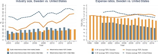
In addition to having unique data on compensation of mutual fund managers, the Swedish setting constitutes a good laboratory to investigate the mutual fund industry. Sweden has one of the deepest and competitive mutual fund sectors in the world. The size of the total mutual fund industry’s AUM relative to gross domestic product (GDP) is one of the highest in the cross-section of countries. Khorana, Servaes, and Tufano (2005) surveyed 58 countries in 2001. According to their data, Sweden’s mutual fund industry represents 31.1% of GDP, ranking 8th out of 58 countries. Moreover, since 2001, the Swedish mutual fund industry has grown tremendously. By 2015, Sweden had almost caught up with the United States in terms of AUM/GDP, as shown in Figure 1. Khorana, Servaes, and Tufano (2005) also calculate the ratio of the AUM in equity funds to the stock market capitalization. For Sweden, this ratio is 23.1% in 2001, ranking it 12th out of 58 countries. The bars in Figure 1 show the evolution of the equity mutual funds’ AUM to stock market capitalization ratio over the previous decade in Sweden and the United States. According to this metric, the Swedish fund industry has also grown tremendously, and is similar in size to that of the United States.
Size and fees of the Swedish mutual fund industry
Data for the United States are from the 2014 Investment Company Factbook and the National Income and Products Accounts. Data for Sweden are from the Swedish Mutual Fund Industry Association and Statistics Sweden.
Sweden also is representative in terms of fund return performances and fees charged in the cross-section of developed countries. Ferreira et al. (2012) study 28 countries from 2001 to 2007. They show that fund performance, measured by quarterly raw returns (1.93%), one-factor alpha (|$-0.80%$|), or four-factor alpha (|$-0.83%$|), in Sweden is close to the cross-country averages (2.07%, |$-0.47%$|, |$-0.60%$|). Flam and Vestman (2017) confirm that Swedish fund alphas are close to their U.S. counterparts. Percentage annual fees of 1.38% are also close to the cross-country average of 1.29%. Figure 1 plots the time series for the total expense ratio (TER) over a longer and more recent sample, again comparing the United States to Sweden. The lines plot equally weighted averages across funds, while the bars plot AUM-weighted averages. Sweden has comparable fees to the United States, especially on an equally weighted basis. The evidence is consistent with Sweden having a competitive mutual fund sector in the international context.
A third piece of international evidence comes from the flow-performance relationship. We confirm in our data (see Appendix C) the strong flow-performance relationship found for Sweden by Ferreira et al. (2012). These authors show a stronger flow-performance relationship in eight countries, including Sweden, than the one for the United States first established by Sirri and Tufano (1998). The convexity of this relationship can result from misspecification of the fractional flow model Spiegel and Zhang, 2013. Our work does not rely on the nature of the flow-performance relationship.
A final piece of evidence speaks to the competitiveness of the market for skilled labor in Sweden. Adams, Keloharju, and Knupfer (2016) study CEO pay in Sweden. Their Figure 2, panel B, shows an elasticity of CEO pay to firm assets of 0.27. They note that this estimate is quite close to the 0.3 estimate reported for U.S. firms. The pay specification they use is the same we employ below, and follows from the assignment model of Gabaix and Landier (2008). This is evidence that the pay culture for skilled labor in Sweden may not be very different from that in the United States. As we show below, Swedish mutual fund managers have an elasticity of pay to revenue that is only half as high as that of Swedish CEOs.
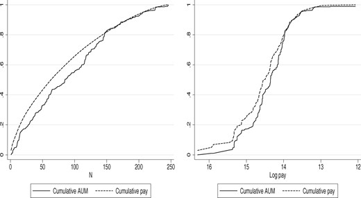
Cumulative labor income and assets under management by income
Both panels plot the cumulative fraction of labor income expressed as a fraction of total labor income paid (dashed line), and cumulative assets under management, expressed as a fraction of total AUM (solid line) for all managers in the last year of our sample, 2015. Managers are ordered from highest to lowest pay on the horizontal axis. The left panel plots the number of managers on the x-axis, while the right panel plots the log pay.
1.2. Three hierarchical levels of data
Our data set has three hierarchical levels: mutual fund companies, which we refer to as firms, mutual funds, and fund managers. This section describes how we measure returns, revenues, and compensation at these various levels of aggregation.
From Morningstar Direct, we obtain the universe of open-ended mutual funds that are available for sale in Sweden or in the Nordic countries. The sample period is from January 1994 until December 2015. The sample includes both active and no longer active funds. The mutual funds have inception dates between 1975 and 2014. We eliminate all funds that have Region of Sale equal to Global Cross-Border or European Cross-Border because those are funds that do not have local operations in Sweden. The sample contains 1,744 funds that belong to 182 fund companies, identified by Morningstar’s variable Firm Name. Some fund companies are subsidiaries of a larger unit, the fund complex, identified by the Morningstar variable Branding Name. Often, the various fund companies in a fund complex operate in different Nordic companies.7 The 182 fund companies form 126 complexes.
Morningstar Direct provides the manager history for each fund. The history contains the first and last names of each manager with a start date and end date. This generates 10,123 non-missing fund manager-year observations for 1,600 funds.8
What makes our data set unique is that we match the managers to their social security numbers, using publicly available sources. This is what allows the match to the tax records that contain the manager income data. We describe the matching procedure in detail in Appendix A.1. For 670 fund managers’ names, we do not find a (reliable) match with a social security number. Many of these names are Finnish, Danish, or Norwegian and likely stem from the inclusion of Nordic cross-border funds. These fund managers are not Swedish taxpayers and do not have a Swedish social security number. For common manager names, we obtain several candidate social security numbers. Based on age, industry, and occupation, we are often able to identify the correct individual. In some cases, too many candidates remain, and we drop such many-to-one matches. Our final estimation sample contains 2,898 fund manager-year observations pertaining to 945 funds and 531 fund managers.
1.2.1 Fund level.
We denote by |$R^{\it gross}_{\it it}$| mutual fund |$i$|’s gross return in month |$t$|. The net return |$R^{net}_{\it it}$| is the gross return minus the total expense ratio, denoted by |${\it TER}_{\it it}$|. |$R^B_{\it it}$| is the fund’s benchmark return. This can be either the return on the benchmark stated in the prospectus or the return from a factor model. We denote by |$R^{\it abn}_{\it it}$| the abnormal return, defined as the return of the fund over the benchmark return before expenses. The fund earns fee revenue (|${\it REV}_{\it it}$|) equal to the product of assets under management at the end of last month times the total expense ratio (annual TER/12). The value added (|$V_{\it it}$|) is defined as in Berk and van Binsbergen (2015) as the product of the AUM of the fund at the end of last month (|${\it AUM}_{it-1}$|) times the difference between the gross return and the benchmark return. Net value-added takes out fund revenue from (gross) value added.
Following the literature, we eliminate money market mutual funds as well as index funds, identified as such by Morningstar or by the word “index” in their name. We also eliminate the four government pension funds that invest public pension money. We believe they are fundamentally different from privately owned mutual funds. The remaining funds belong to one of five categories based on the Morningstar GlobalBroadCategoryGroup variable: Equity, Allocation (mix of stocks and bonds), Fixed Income, Alternatives, and a Rest category, which combines commodity funds, miscellaneous funds, and funds where the category variable is missing. The Alternatives category contains Currency, Long/Short Equity, Market Neutral, Multi-Alternative, and Other Alternative funds. This category mainly consists of hedge funds which in Sweden are allowed to market themselves directly toward the general public. Many of the Equities and Fixed Income funds specialize in specific investment regions or in specific industries.9 Most of the miscellaneous funds in the Rest category are either capital protected or guaranteed, a common type of structured product in Europe.
We retrieve monthly time series of AUM from Morningstar, calculate monthly revenue, and form annual counterparts by summing the monthly values.10 Several funds have multiple share classes. AUM is available per share class. We aggregate those share classes into a single fund (identified by Morningstar’s variable FundId). We convert AUM values in other currencies than SEK into SEK when necessary. Similarly, we obtain total expense ratios per share class and aggregate them across share classes using AUM weights. We complement the annual AUM and TER time series from Morningstar Direct with two additional sources, Bloomberg and some hand-collected data obtained from AMF Fonder.11 Our final data set has 5,668 fund-year observations. In 1994, the aggregate AUM among the sample funds is 2.6 billion SEK. Aggregate AUM increases to 1,772.9 billion SEK by 2015. All SEK amounts are expressed in 2012 real SEK. The average SEK/USD exchange rate over the 1994–2015 period is 7.5.
Summary statistics for the funds employed in our main regression analysis are reported in Table 1. Panel A shows that the average fund has AUM of 2,300 million SEK, or about
Summary statistics at the fund level
| 10% | 25% | 50% | 75% | 90% | Mean | Sd | N | |
|---|---|---|---|---|---|---|---|---|
| A. Fund AUM and TER | ||||||||
| |${\it AUM}_{i}$| (mio. SEK) | 63.3 | 199.9 | 698.3 | 2,424.8 | 6,600.3 | 2,305.7 | 3,976.9 | 5,545 |
| |${\it TER}_{i}$| (%) | 0.50 | 0.77 | 1.42 | 1.70 | 2.21 | 1.36 | 0.68 | 5,609 |
| |${\it REV}_i$| (mio. SEK) | 0.7 | 2.4 | 7.9 | 28.5 | 80.4 | 27.6 | 47.7 | 5,518 |
| |$\log({\it REV}_{i})$| | 13.5 | 14.7 | 15.9 | 17.2 | 18.2 | 15.8 | 1.8 | 5,518 |
| B. Fund performance (%) | ||||||||
| |$\log (1+R_{i}^{\it exc})$| | –20.2 | –2.2 | 6.9 | 18.1 | 27.9 | 5.2 | 21.6 | 4,484 |
| |$\log (1+R_{i}^{\it abn})$| | –8.6 | –2.9 | 0.5 | 4.1 | 9.8 | 0.6 | 8.5 | 4,467 |
| |$\log (1+R_{i}^{\it abn,CAPM})$| | –10.0 | –3.9 | 0.3 | 4.0 | 10.1 | 0.1 | 9.3 | 4,460 |
| |$\log (1+R_{i}^{\it abn,FF3})$| | –9.3 | –3.3 | 0.7 | 4.4 | 9.6 | 0.4 | 8.8 | 4,460 |
| |$\log (1+R_{i}^{\it abn,GF5})$| | –8.4 | –3.8 | 0.1 | 3.7 | 9.7 | 0.2 | 8.1 | 4,393 |
| |$ValueAdded_{i}$| (mio. SEK) | –90.2 | –15.0 | 1.3 | 27.9 | 142.6 | 26.9 | 225.5 | 4,416 |
| C. Manager characteristics | ||||||||
| |${\it Age}_m$| | 33 | 37 | 42 | 48 | 52 | 42 | 7.5 | 2,898 |
| |${\it Exper}_m$| | 1.0 | 2.4 | 4.8 | 8.1 | 12.2 | 5.9 | 4.7 | 2,898 |
| |${\it Edu}_m$| | 12 | 15 | 15 | 16 | 16 | 15 | 2 | 2,898 |
| |${\it Coman}_m$| | 0.00 | 0.00 | 0.12 | 1.00 | 1.00 | 0.45 | 0.48 | 2,898 |
| |$ {\it Teams}_m$| | 0.00 | 0.00 | 0.92 | 1.00 | 3.00 | 1.21 | 2.26 | 2,898 |
| |${\it TeamSize}_m$| | 0.00 | 0.00 | 0.14 | 1.00 | 2.00 | 0.72 | 1.03 | 2,898 |
| |${\it NumCat}_m$| | 1.0 | 1.0 | 1.0 | 1.0 | 2.0 | 1.2 | 0.5 | 2,898 |
| D. Manager income (1000s of SEK) | ||||||||
| |$L_m$| | 510.6 | 788.3 | 1,206.5 | 1,806.7 | 2,739.8 | 1,559.3 | 1,522.5 | 2,898 |
| |$D_m$| | 0.0 | 0.0 | 4.2 | 41.8 | 450.6 | 813.0 | 8,730.1 | 2,898 |
| |$Y_m$| | 548.1 | 856.4 | 1,341.5 | 2,042.8 | 3,427.1 | 2,372.3 | 8,864.5 | 2,898 |
| E. Firm level | ||||||||
| |${\it AUM}_{f}$| (bio. SEK) | 0.1 | 0.7 | 3.7 | 17.7 | 65.6 | 24.5 | 61.2 | 929 |
| |${\it TER}_{f}$| (%) | 0.69 | 1.00 | 1.26 | 1.64 | 2.40 | 1.40 | 0.66 | 928 |
| |${\it REV}_f$| (mio. SEK) | 2.0 | 9.9 | 48.0 | 208.4 | 693.1 | 278.0 | 670.2 | 928 |
| |$\log({\it REV}_f)$| | 14.5 | 16.1 | 17.7 | 19.2 | 20.4 | 17.6 | 2.2 | 928 |
| |${\it Profit}_f$| (mio. SEK) | –1.9 | 0.3 | 10.1 | 48.3 | 152.1 | 57.5 | 152.1 | 646 |
| |${\it Profit}_f^{+}$| (mio. SEK) | 1.1 | 4.5 | 22.7 | 68.5 | 217.3 | 76.0 | 168.5 | 498 |
| No. of funds / year | 1.0 | 2.0 | 5.0 | 11.0 | 31.0 | 11.2 | 17.7 | 929 |
| No. of managers / year | 1.0 | 2.0 | 3.0 | 9.0 | 20.0 | 7.6 | 10.5 | 929 |
The sample contains all fund-year observations that are used in our main analysis (Table 2). Panels A and B provide summary statistics at the fund level. A fund-year observation is included if it is managed by a manager in our sample in that year. We winsorize the performance variables, AUM, TER, and REV, at the 1% and 99% levels. Panels C and D contain summary statistics at the manager level. We do not winsorize income or characteristics variables. Panel E aggregates the fund-year observations into firm-year observations.
Sensitivity of pay to size and performance
| (1) | (2) | (3) | (4) | (5) | (6) | |
|---|---|---|---|---|---|---|
| |$\log (L_{\it m,t})$| | |$\log (L_{\it m,t})$| | |$\log (L_{\it m,t})$| | |$\log (L_{\it m,t})$| | |$\log (L_{\it m,t})$| | |$\log (L_{\it m,t})$| | |
| |$\log ( {\it REV}_{\it m,t} )$| | 0.153*** | 0.141*** | 0.123*** | |||
| (0.0184) | (0.0194) | (0.0239) | ||||
| |$\log (1+R^{\it abn}_{\it m,t-1})$| | 0.340* | 0.407** | 0.0913 | |||
| (0.206) | (0.189) | (0.143) | ||||
| |${\it Exper}_{\it m,t-1}$| | 0.0323*** | 0.0961** | 0.0570*** | 0.121** | ||
| (0.0118) | (0.0482) | (0.0123) | (0.0569) | |||
| |${\it Exper}^2_{\it m,t-1}$| | –0.000533 | –0.0000195 | –0.00119*** | –0.000731 | ||
| (0.000408) | (0.000755) | (0.000446) | (0.000721) | |||
| |${\it Age}_{\it m,t-1} $| | 0.177*** | 0.0942 | 0.175*** | 0.0994 | ||
| (0.0292) | (0.0676) | (0.0278) | (0.0751) | |||
| |${\it Age}^2_{\it m,t-1}$| | –0.00191*** | –0.00153*** | –0.00193*** | –0.00156*** | ||
| (0.000351) | (0.000544) | (0.000327) | (0.000584) | |||
| |${\it Edu}_{\it m,t-1} $| | 0.00938 | –0.0264 | 0.0164 | –0.00132 | ||
| (0.0145) | (0.0493) | (0.0150) | (0.0500) | |||
| |$ {\it Finance}_{\it m,t-1}$| | 0.259** | 0.255*** | 0.335*** | 0.280*** | ||
| (0.106) | (0.0572) | (0.0892) | (0.0654) | |||
| |${\it Coman}_{\it m,t-1}$| | –0.223*** | 0.0626 | –0.310*** | 0.00874 | ||
| (0.0830) | (0.106) | (0.0830) | (0.113) | |||
| |$ {\it Teams}_{\it m,t-1}$| | –0.0261** | 0.00121 | 0.00781 | 0.0166* | ||
| (0.0103) | (0.00855) | (0.0104) | (0.00915) | |||
| |$ {\it TeamSize}_{\it m,t-1}$| | 0.114*** | –0.0110 | 0.0952** | –0.0346 | ||
| (0.0384) | (0.0466) | (0.0391) | (0.0504) | |||
| |$ {\it NumCat}_{\it m,t-1}$| | 0.0988 | 0.0934* | 0.118* | 0.151*** | ||
| (0.0691) | (0.0511) | (0.0694) | (0.0553) | |||
| Constant | 10.96*** | 7.173*** | 10.35*** | 13.59*** | 9.450*** | 11.64*** |
| (0.321) | (0.595) | (1.834) | (0.155) | (0.632) | (2.192) | |
| Manager FE | No | No | Yes | No | No | Yes |
| Year FE | Yes | Yes | Yes | Yes | Yes | Yes |
| Category FE | No | Yes | Yes | No | Yes | Yes |
| |$N$| | 2,898 | 2,898 | 2,898 | 2,898 | 2,898 | 2,898 |
| Adjusted \(R^{2}\) | 0.139 | 0.229 | 0.614 | 0.023 | 0.146 | 0.594 |
| Standardized Revenue and Performance | ||||||
| |$ \log ( {\it REV}_{\it m,t} )_{\it std}$| | 0.281*** | 0.253*** | 0.187*** | |||
| (0.0365) | (0.0362) | (0.0468) | ||||
| |$ \log (1+R^{\it abn}_{\it m,t-1} )_{\it std}$| | 0.0298 | 0.0290 | –0.00328 | |||
| (0.0198) | (0.0193) | (0.0154) | ||||
The dependent variable is annual log labor income of the fund manager. The independent variables are a constant, log revenue generated by the manager in that same year, log annual fund returns at the manager level over the past year, manager experience in years working as a fund manager, experience squared, manager age, manager age squared, years of education, indicator variable for finance or economics degree, the fraction of funds that are co-managed with other managers, the number of management teams the manager serves on, the size of management teams, and the number of different investment categories that the manager’s funds belong to. All specifications include year fixed effects. Some specifications additionally include investment category fixed effects and manager fixed effects. When category fixed effects are included, the Equity category is omitted. The bottom panel estimates a separate set of regressions, which replaces the variables in the first two rows by standardized versions of those same variables (denoted by the subscript “std”). The scaling is done by investment category and results in a variable that is mean zero and has standard deviation of one. All standard errors are clustered at the manager level.
We obtain monthly net fund returns from Morningstar. To calculate gross monthly returns, we add TER/12. All returns are converted into SEK. Excess returns are calculated by subtracting the one-month STIBOR (Stockholm Interbank Offered Rate) rate. We calculate annual log returns by summing log monthly returns. Panel B of Table 1 shows that the average fund has a log excess annual return of 5.2%; the median is 6.9%. The interquartile range is large, ranging from –2.2% to 18.1%.
As our main measure of performance, we use the gross abnormal return or “alpha” relative to the stated benchmark return in logs, |$\log(1+R^{\it abn}_i)$|. This is a simple measure of gross alpha. Gross returns rather than net returns are what matter in the relationship between owners and managers. In order to construct it, we require a benchmark for each fund in our sample.
Morningstar reports a Primary Prospectus Benchmark for 74% of our funds. Some funds have linear combinations of indices as their benchmark. There are more than 300 different benchmark indices present in our sample. We find monthly return information for most of them on Morningstar, Bloomberg, and Datastream. For funds with no assigned benchmark or irretrievable benchmark, we assign a benchmark by hand.12 We express all benchmark returns in SEK. The median annual log (gross) abnormal return is 0.5%. The distribution has a large 8.5% standard deviation. The interquartile range is |$-2.9%$| to 4.1%. Net abnormal returns (after expenses, not reported) are slightly negative on average, consistent with the evidence for the United States.
We explore four alternative measures of abnormal returns. They are the CAPM alpha, the Fama-French three-factor alpha, the global five-factor alpha, and gross value added. For the Equity, Alternative, and Allocation categories we use the Swedish stock market index return (SIXPRX) in excess of the one-month STIBOR rate as the CAPM market factor. For the Fixed Income and Other categories, we use the Swedish government bond index return (OMRX) in excess of the one-month STIBOR rate as the CAPM market factor.13 The three-factor Fama-French model has the stock market factor, the size factor (SMB), and the value factor (HML), constructed from all Swedish stocks. We also consider a global five-factor model. For the Equity, Alternative, and Allocation categories, the five factors are five excess returns on different international equity baskets.14 For the Fixed Income and Other categories, the five factors are five international bond factor excess returns.15 Gross value added, defined in Equation (4), uses the stated benchmark and is expressed in millions of SEK. The last four rows of panel B of Table 1 show the distribution of these alternative performance measures across funds. The average gross CAPM alpha is 0.1% and has an even wider dispersion than the main abnormal return measure. Average three- and five-factor alphas are also close to zero with similar dispersion. Median gross value added is 1.3 million SEK. It is negative for slightly less than half the fund-year observations, and has a right tail of 143 million SEK at the 90th percentile.
1.2.2 Manager level.
Panel C of Table 1 reports manager characteristics for the final sample of manager-year observations.17 The average and median age is 42 years. Their average years of experience managing mutual funds is 5.9, with a standard deviation of 4.7 years. They have 15 years of formal education on average, which reflects having obtained a college degree. The manager at the 10th percentile has only completed high-school whereas the top 25% have completed at least one additional one-year degree. We calculate the fraction of manager |$m$|’s funds that are co-managed (|${\it Coman}$|), the average number of teams manager that |$m$| is on in a given year (|${\it Teams}$|), and the average team size, excluding the manager herself, for the funds managed by manager |$m$| (|${\it TeamSize}$|). The median manager co-manages 12% of her AUM, is on 0.92 teams, and has 0.14 teammates. There is nontrivial dispersion in all of these variables. Managers mostly manage funds within a single investment category: the average number of investment categories in manager |$m$|’s portfolio of funds (|${\it NumCat}$|), in a given year, is typically 1, with less than 20% managing assets in more than one category.
Our main outcome variable is the labor income (|$L_{\it mt}$|) of a mutual fund manager |$m$| in year |$t$|. Labor income is defined as regular salary and benefits plus business income, before taxes. Including business income is useful for cases where the manager is running a fund for a fund family as a self-employed consultant. From the perspective of Swedish tax legislation, any bonus pay from the employer is considered as labor income and included in our measure. Panel D reports income measures in thousands of Swedish kronor (SEK). The median fund manager earns 1.2 million SEK in labor income (about
While there is substantial inequality in labor income in our sample, it is not the case that a handful of managers account for most of the labor income or the assets under management. To see this, Figure 2 plots the cumulative fraction of labor income and assets under management for all managers in the last year of our sample, 2015. Managers are ordered from highest to lowest pay on the horizontal axis. The left panel plots the number of managers on the x-axis, while the right panel plots the log pay. The middle one hundred managers out of 246 managers, whose log labor income lies between 13.8 and 14.4, account for one-third of the income paid and over 40% of AUM. These managers manage a significant amount of assets.
As a second measure of pay, we add dividend income (|$D_{\it m,t}$|) to labor income to obtain total income (|$Y_{\it m,t}$|). The advantage of including dividend income is that we obtain a more comprehensive measure of pay. Some mutual fund managers may be compensated with stock or may have personal companies that are shareholders in the mutual fund family. That personal company then pays dividends to the individual. These payments reflect, at least in part, the efforts and talents of the manager. Payments through dividends may also be a more tax-efficient way of providing compensation.18 There are two disadvantages. We only have data on total dividend income, so that dividend income includes dividends from all other equity positions the manager has, including many that have no relationship to his or her employment. Second, the timing of the dividend payments from the personal company to the individual is arbitrary and may break the link between performance in year |$t-1$| and total pay in year |$t$|. The median fund manager has very little dividend income. But the distribution is extremely right-skewed.19 Dividend income is 0.5 million at the 90th percentile and 0.8 million on average. The standard deviation is 8.7 million. In other words, we have some extremely high-earning individuals in our data set, even by U.S. standards. Total income averages 2.4 million SEK or
1.2.3 Firm level.
Each fund company or firm offers multiple funds and employs many managers. Panel E of Table 1 aggregates up from the fund to the firm level. Our sample contains about 930 unique firm-year observations. The average AUM at the firm level is 25 billion SEK, the median is 4 billion. The average TER at the firm level remains around 1.4%. Firm revenue averages 280 million SEK. From the Serrano accounting data base, we obtain net firm profits. Median firm profits are 11 million SEK, mean profits 58 million SEK. We define |${\it Profit}^+$| as the positive part of profits.20 It is only defined for firm-year observations with positive profits. The average firm has 11.2 funds and employs 7.6 managers in a given year in our data set, while 10% percent of firm-year observations have more than 31 funds and more than 20 fund managers.
2. Manager-level Determinants of Compensation
This section investigates the manager-level determinants of labor income in the cross-section of mutual fund managers. The next section argues that firm-level characteristics co-determine fund manager compensation.
2.1. Pay-revenue sensitivity
2.1.1 Empirical specification.
In our first set of results, we ask whether managerial pay depends on the size of the fund(s) managed and the performance of the fund(s). As our main measure of size we use the fee revenue of the funds managed by a given manager. Fee revenue is easily measurable, and therefore contractible, and it is a measure of the sales revenue directly associated with the activities of the manager. As indicated above, manager-level revenue is the assets under management times total expense ratio, calculated for each month, and then added up across months. Since AUM and revenue change throughout the year, we want to allow for revenue to affect pay contemporaneously.21 Fund performance is lagged because the bonus received in year |$t$| typically reflects performance in the previous calendar year.
2.1.2 Sensitivity of pay to revenue.
To estimate the pay-revenue sensitivity (PRS) coefficient |$\beta$|, we set |$\gamma=0$| in Equation (11). In Column (1) of Table 2, we only include a constant and log revenue. We find an elasticity of pay to size of 0.153, which is measured precisely (standard error of 0.018). A 1% increase in the revenues from the funds a manager operates increases her pay by about 0.15 %. This specification rejects the null hypothesis of a compensation that is independent of fund size. Log revenue accounts for a substantial 13.9% of the overall variation in pay.
On the one hand, this result suggests that the owners and the managers of mutual funds have incentives that are aligned, in that both of their payoffs increase in fund revenue. It also shows that the manager-specific fund revenue matters for compensation.
On the other hand, large variation in fund revenue is associated with only modest variation in manager pay. A doubling of revenue from funds under management (increase by 100% or 1 log unit) increases pay by 15%. Fund managers capture only a small share of the additional fund revenues. To illustrate, consider a simple example with amounts converted to U.S. dollars. Average manager-level revenue is about
To further gauge the economic magnitude of the effect, we standardize log revenue by dividing by the cross-sectional standard deviation. Because fixed income and equity mutual funds may have different revenue distributions, we standardize investment category by category.23 We then reestimate the same regression specification but with standardized log revenue as independent variable. The main coefficients of interest are reported in the bottom panel of Table 2. A one-standard-deviation increase in log revenue is associated with a 28.1% increase in pay. This represents a 0.4-standard-deviation change in log labor income.
In Column (2), we add control variables |$X_{\it m,t-1}$|. These are measured annually and include: the manager’s experience in years worked as a fund manager (|${\it Exper}$|), experience squared (|${\it Exper}^2$|), age of the manager (|${\it Age}$|), age squared (|${\it Age}^2$|), years of education (|${\it Edu}$|), an indicator variable for a degree with a finance specialization (|${\it Finance}$|),24 the fraction of manager |$m$|’s funds that are co-managed (|${\it Coman}$|), the average number of teams manager |$m$| is on in a given year (|${\it Teams}$|), the average team size excluding the manager herself for the funds managed by manager |$m$| (|${\it TeamSize}$|), the average number of categories manager |$m$| runs (|${\it NumCat}$|), and investment category fixed effects. The equity funds category is the omitted category.
The control variables enter with the expected sign, and several are statistically significant. One year of additional experience as a fund manager increases pay by 3.2%. The returns to experience are concave. Older managers make more, and the returns to age are strongly concave, after controlling for experience. On average, a 45-year-old manager makes 7.3% more than a 40-year-old manager, using both linear and quadratic terms. An extra year of education increases pay by 1%. This effect is not significant because we have too little variation in years of education. Having a specialized finance education boosts pay by an economically and statistically significant 25.9%. A manager who co-manages all her funds has 22.3% lower pay than a manager who manages all funds by herself. Each additional team subtracts 2.6% from pay. Larger teams are associated with higher pay; each team member adds 11.4% to pay. Finally, a manager active in more than one investment category makes 9.9% per additional category, but this effect is imprecisely estimated. The specification includes investment category (asset class) fixed effects. The controls increase the |$R^2$| of this regression to 22.9%, a gain of 9.1 percentage points.
Taking into account controls does not change the sensitivity of pay to revenue by much. The elasticity point estimate is 0.141 and remains precisely estimated. The bottom panel of the table shows that a one-standard-deviation increase in revenue (relative to the other funds in the same category) increases pay by 25.3% once controls are included.
In Column (3) we add manager fixed effects. The sensitivity of pay to revenue is now identified from time-series variation for a given manager. Years in which the manager’s funds generate more fee revenue are years of higher managerial pay. The elasticity estimate drops only modestly to 0.123 and remains precisely estimated. A one-standard-deviation increase in revenue increases pay by 18.7%. Comparing the point estimates on size in Columns (2) and (3), we conclude that most of the variation in pay related to fund revenue is not driven by cross-sectional variation in constant skill levels.25
2.1.3 Log-log specification.
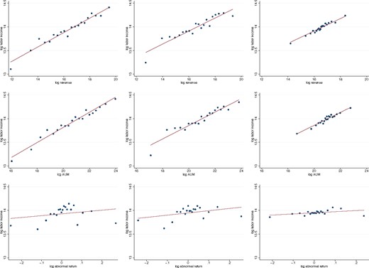
The top row of Figure 3 shows the relationship between log fund revenue (one the horizontal axis) and log pay (on the vertical axis). Each of the 20 points represents 5% of the observations. The best-fitting line through the points is also shown; its slope is the elasticity of pay to size. The left picture corresponds to Column (1) of Table 2, the middle picture shows the slope after including the controls and corresponds to Column (2), while the right panel controls for manager fixed effects in addition. The graphs make clear that a log-log specification for revenue and compensation fits the data very well.26 This log-log specification comes out of the matching framework of Gabaix and Landier (2008) and is also used for Swedish CEO pay by Adams, Keloharju, and Knupfer (2016).
Elasticity of pay to revenue, assets under management, and performance
Each dot pertains to 5% of all observations. The top row plots log revenue |$\log\left({\it REV}_{\it mt}\right)$| against log compensation |$\log\left(L_{\it mt}\right)$|, the middle row plots log AUM |$\log\left({\it AUM}_{\it mt}\right)$| against log compensation and the bottom row plots log abnormal return |$\log\left(1+R^{\it abn}_{\it mt}\right)$| against log compensation. The left panels are the raw data. The middle panel removes the effect of the control variables, year fixed effects, and category fixed effects. The right panels additionally remove manager fixed effects.
The middle panels in Figure 3 replace log revenue by log of assets under management. This alternative size measure of size displays a very similar linear-in-logs relationship to managerial pay. Given the similarity, we proceed with revenue as our preferred measure of size.
2.1.4 Comparison to Berk and Green.
To contextualize the pay-revenue sensitivity estimate of 0.15, it is useful to compare it with the PRS in a benchmark model. The frictionless delegation model of Berk and Green (2004) is a natural benchmark. In that model, each firm runs one fund. The fund manager has unknown ability to the owner and investors, and realizations of abnormal returns are combined with priors to form posterior beliefs on the skill (alpha) of the manager. The model assumes that there are no frictions in the second layer of delegation between the firm owner and the firm manager.27 Equivalently, managerial pay is proportional to firm revenue. Trivially, a regression of log labor income on log revenue delivers a PRS of 1 and an |$R^2$| of 100%. Moreover, controlling for manager fixed effects should capture the manager’s alpha quite well, especially for more experienced managers for whom the posterior precision of beliefs about alpha is high. Our results indicate a much lower PRS than 1, a much lower |$R^2$| than 100%, and a PRS estimate that is little affected by the inclusion of manager fixed effects. The model comparison provides further support for the claim that the estimated PRS is small.
2.2. Pay-performance sensitivity
A second natural manager-level candidate determinant of pay is the return performance of the manager. We define performance as the abnormal return, the manager’s gross return over the stated benchmark, and expressed in logs. We lag the abnormal return under the hypothesis that the return from the past year is what determines the bonus in the current year.
We estimate |$\gamma$| in Equation (11), and set |$\beta=0$|. Column (4) of Table 2 contains the simplest specification without controls or manager fixed effects. We find a baseline PPS of 0.34. The point estimate is significant at the 10% level. Variation in abnormal returns explains only 2.3% of variation in pay. The bottom panel indicates that a one-standard-deviation increase in abnormal return, relative to the other funds in the investment category, increases pay by 2.98%.
A one-percentage-point increase in the log annual abnormal return of a manager increases pay by 0.34%. This is a very small effect. Log pay increases from 13.59 when the net abnormal return is zero to 13.5934 (|$13.59 + 0.01 \times 0.34$|) when the annual abnormal return is 1%. At 7.5 SEK per USD, the (nontrivial) increase of 1% point in abnormal return represents an annual pay increase of a paltry
Column (5) adds the control variables. The performance sensitivity coefficient increases in magnitude to 0.407 as well as in significance (5% level). There is some evidence that managerial pay is linked to the abnormal returns, after controlling for experience, age, education, and so on. But the economic magnitude of the pay-for-performance sensitivity remains small. Even though performance-based pay may be prevalent, as suggested by Ma, Tang, and Gomez (2016), the importance of the performance-based component of compensation appears modest at best. One possibility we explore is that pay is tied to additional lags of abnormal returns.
Column (6) adds manager fixed effects. The semielasticity drops to 0.093 and loses significance. Whatever PPS we find is largely driven by cross-sectional variation rather than time-series variation for a given manager.
2.2.1 Log-log specification.
The bottom row of Figure 3 visually confirms the weak relationship between performance (log gross abnormal return on the horizontal axis) and log pay (on the vertical axis). The slope of the best-fitting line through the points is the semi-elasticity of pay to performance. The left picture corresponds to Column (4) of Table 2, the middle picture shows the slope after including the controls and corresponds to Column (5), while the right panel controls for manager fixed effects in addition (Column 6). The graphs make clear that a linear-in-logs specification for abnormal return, and pay does not fit the data that well.28 We explore different nonlinear specifications in Section 4.1.
2.2.2 Comparison to Berk and Green.
To gauge how small the estimated PPS is, we return to the Berk and Green model. We simulate their benchmark calibration and estimate a panel regression of log compensation on the lagged log abnormal return in simulated data. We find a PPS estimate of 1.61 without and 0.75 with fixed effects. The estimates are a factor four to six times larger than the estimates in the data. In a world with uncertainty about managerial skill, abnormal returns are informative to investors and managers alike. Investors reward high-performance fund managers with flows and fee revenues. The data suggest much weaker responses than in the model. Simulation and calibration details are in Appendix B.
2.3. Revenue as measure of skill
In this section, we investigate the relationship between pay and fee revenue further. Specifically, we address the possibility that pay is sensitive to fee revenue because revenue contains performance-related components that are associated with pay. Managers with higher abnormal returns mechanically grow their AUM, and hence their fee revenue; they may attract more investor flows (Sirri and Tufano 1998); may be able to charge higher expense ratios (Warner and Wu 2011); and may be promoted by firm owners to run more or larger funds (Berk, van Binsbergen, and Liu 2017). However, revenue could also differ across funds and over time for reasons unrelated to the manager’s investment skill. Firm-level variables, such as advertising/marketing, distribution network, or common research infrastructure, could affect fund revenue. So could managerial talents unrelated to investment skill, such as fundraising ability or people management skills. Finally, fund flows could result from portfolio rebalancing or from investors responding to benchmark returns (Del Guercio and Reuter 2014).
To remove the performance-related component of revenue, we regress log revenue on log abnormal return. The residual of this regression is the component of log revenue that is orthogonal to performance, |$\log({\it REVorth}_{\it m,t})$|. Column (2) of Table 3 orthogonalizes log revenue in year |$t$| to both the current year’s abnormal return, |$\log(1+R^{\it abn}_{\it m,t})$|, and the previous year’s, |$\log(1+R^{\it abn}_{\it m,t-1})$|. It shows that the sensitivity of pay to revenue is essentially unaffected. Compared with our benchmark specification, repeated for convenience in Column (1), the PRS mildly increases from 0.141 to 0.144. In Column (3), log revenue is orthogonalized to two additional lags of abnormal return, |$\log(1+R^{\it abn}_{\it m,t-2})$| and |$\log(1+R^{\it abn}_{\it m,t-3})$|. The PRS remains stable at 0.134.29 In sum, the PRS is barely affected even after the effect of manager-level abnormal returns is purged from revenue.
Decomposing the effect of revenue on pay
| (1) | (2) | (3) | (4) | (5) | (6) | (7) | |
|---|---|---|---|---|---|---|---|
| |$\log (L_{\it m,t})$| | |$\log (L_{\it m,t})$| | |$\log (L_{\it m,t})$| | |$\log (L_{\it m,t})$| | |$\log (L_{\it m,t})$| | |$\log (L_{\it m,t})$| | |$\log (L_{\it m,t})$| | |
| |$ \log ( {\it REV}_{\it m,t} )$| | 0.141*** | 0.140*** | |||||
| (0.0194) | (0.0195) | ||||||
| |$ \log ({\it REVorth}_{\it m,t})$| | 0.144*** | 0.134*** | 0.144*** | 0.144*** | 0.130*** | ||
| (0.0194) | (0.0257) | (0.0193) | (0.0193) | (0.0255) | |||
| |$ \log (1+R^{\it abn}_{\it m,t})$| | 0.0646 | 0.253 | |||||
| (0.151) | (0.194) | ||||||
| |$ \log (1+R^{\it abn}_{{\it m,t-}1})$| | 0.148 | 0.327* | 0.325* | 0.586** | |||
| (0.176) | (0.174) | (0.170) | (0.236) | ||||
| |$ \log (1+R^{\it abn}_{{\it m,t-}2})$| | 0.583*** | ||||||
| (0.200) | |||||||
| |$ \log(1+R^{\it abn}_{{\it m,t-}3})$| | 0.274* | ||||||
| (0.158) | |||||||
| Constant | 7.173*** | 9.509*** | 9.074*** | 7.212*** | 9.563*** | 9.561*** | 9.141*** |
| (0.595) | (0.639) | (0.894) | (0.602) | (0.646) | (0.645) | (0.904) | |
| Manager FE | No | No | No | No | No | No | No |
| Year FE | Yes | Yes | Yes | Yes | Yes | Yes | Yes |
| Category FE | Yes | Yes | Yes | Yes | Yes | Yes | Yes |
| Controls | Yes | Yes | Yes | Yes | Yes | Yes | Yes |
| Firm FE | No | No | No | No | No | No | No |
| |$N$| | 2,898 | 2,883 | 1,932 | 2,898 | 2,883 | 2,883 | 1,932 |
| Adjusted |$R^{2}$| | 0.229 | 0.233 | 0.182 | 0.229 | 0.234 | 0.234 | 0.190 |
See Table 2. The second, fifth, and sixth columns use as the independent variable the part of log revenue that is orthogonal to abnormal returns at time |$t$| and |$t-1$|. The third and seventh columns additionally orthogonalize revenue to abnormal returns at times |$t-2$| and |$t-3$|.
Next, we ask how the pay-performance sensitivity is affected by the removal of the performance-related components of revenue. Columns (4)–(7) of Table 3 contain the results. Column (4) estimates Equation (11) as a reference point, and finds a PRS of 0.140 and a PPS of 0.148, similar to the estimates in Table 2. Column (5) shows that when revenue has been orthogonalized to current and lagged abnormal return, the PPS increases from 0.148 to 0.327 and turns marginally significant. Column (6) adds the contemporaneous abnormal return, which does not alter the estimates. In Column (7), we use the revenue measure that has been orthogonalized to current and three years’ worth of lagged abnormal returns instead, and include all abnormal return terms. The main PRS coefficient increases further to 0.586 and becomes significant at the 5% level. We discuss the effect of the additional lags of returns in Section 2.4. In sum, the sensitivity of pay to performance increases once the abnormal return term captures not only the direct effect of higher return on compensation (the bonus part of pay that is tied to performance), but also the indirect effects of higher abnormal return on revenue (part of the pay tied to revenue). Nevertheless, the economic effect remains very small, with a one-percentage-point increase in abnormal return resulting in a mere 0.586% increase in pay.
Appendix C explores which components of revenue are responsible for the undiminished sensitivity of pay to orthogonalized revenue. It finds nonzero elasticities of pay to several of these components, including lagged revenues, TER growth, benchmark returns, inflows unrelated to performance, and AUM from funds newly assigned to a manager, after these components have been orthogonalized to performance.
2.4. Longer performance evaluation periods
Since returns and abnormal returns are noisy measures of investment skill, performance-based pay may depend not only on last year’s compensation but on longer lags of abnormal returns. Two pieces of empirical evidence are consistent with this conjecture. U.S. mutual funds report mean and median performance evaluation periods of three years.30 Since 2009, new European-level regulation came into place stipulating that a fraction of variable pay must be postponed for three years. Theoretically, fund owners and investors who are learning about a fund manager’s investment skill would only gradually update their posterior about skill.
Table 4 extends our baseline specification for log labor income, reprised in Column (1), by including one or two additional lags of abnormal returns. This is done in Columns (4) and (6). Twice-lagged abnormal returns enter significantly with an estimated elasticity of 0.33. Thrice-lagged returns in Column (6) are imprecisely estimated at 0.19. The last column replaces revenue by revenue orthogonalized to current and three lags of abnormal returns. As explained above, this reallocates the performance-related components of revenue to the abnormal return terms. The PPS coefficients are 0.61, 0.57, and 0.29, all different from zero. While these coefficients are larger and more significant, the economic magnitude of the PPS remains modest at best. A one-percentage-point abnormal return in each of the past three years, which is a nontrivial feat in light of the weak evidence on performance persistence, increases pay by less than 2%.31 Simulations from the Berk and Green model with lagged abnormal returns confirm that our PPS coefficients are low; they are more than 50% larger in the model than in the data. Appendix B contains the details.
Longer evaluation periods
| (1) | (2) | (3) | (4) | (5) | (6) | (7) | |
|---|---|---|---|---|---|---|---|
| |$\log (L_{\it m,t})$| | |$\log (L_{\it m,t})$| | |$\log (L_{\it m,t})$| | |$\log (L_{\it m,t})$| | |$\log (L_{\it m,t})$| | |$\log (L_{\it m,t})$| | |$\log (L_{\it m,t})$| | |
| |$\log ({\it REV}_{\it m,t})$| | 0.140*** | 0.143*** | 0.135*** | 0.141*** | 0.132*** | 0.131*** | |
| (0.0195) | (0.0220) | (0.0256) | (0.0222) | (0.0256) | (0.0255) | ||
| |$\log({\it REVorth}_{\it m,t})$| | 0.131*** | ||||||
| (0.0256) | |||||||
| |$\log (1+R^{\it abn}_{{\it m,t-}1})$| | 0.148 | 0.276 | 0.348 | 0.278 | 0.348 | 0.366 | 0.611** |
| (0.176) | (0.214) | (0.248) | (0.214) | (0.249) | (0.253) | (0.246) | |
| |$\log (1+R^{\it abn}_{{\it m,t-}2} )$| | 0.330** | 0.452** | 0.462** | 0.573*** | |||
| (0.163) | (0.193) | (0.197) | (0.196) | ||||
| |$\log (1+R^{\it abn}_{{\it m,t-}3})$| | 0.198 | 0.286* | |||||
| (0.157) | (0.160) | ||||||
| Constant | 7.212*** | 6.939*** | 6.871*** | 7.034*** | 6.904*** | 6.969*** | 9.136*** |
| (0.602) | (0.722) | (0.866) | (0.732) | (0.868) | (0.876) | (0.902) | |
| Manager FE | No | No | No | No | No | No | No |
| Year FE | Yes | Yes | Yes | Yes | Yes | Yes | Yes |
| Category FE | Yes | Yes | Yes | Yes | Yes | Yes | Yes |
| Controls | Yes | Yes | Yes | Yes | Yes | Yes | Yes |
| Firm FE | No | No | No | No | No | No | No |
| |$N$| | 2,898 | 2,411 | 1,932 | 2,411 | 1,932 | 1,932 | 1,932 |
| Adjusted |$R^{2}$| | 0.229 | 0.218 | 0.188 | 0.219 | 0.190 | 0.190 | 0.190 |
See Table 2. We include additional lags of fund abnormal return. Columns (1),(2), and (3) differ by the number of manager-year observations. So do Columns (4) and (5). These comparisons allow us to gauge the importance of sample selection. Column (2) reestimates the same specification as in Column (1) but limits the sample to the manager-year observations for which we have both one- and two-year lagged abnormal return. Columns (3) and (5) restrict the sample to those observations for which we also have three-year lagged returns.
Despite the weak effect, the PPS estimates are likely upward biased due to survivorship bias. As more lagged returns are added, the sample shrinks, and the remaining manager-year observations have better average performance. To demonstrate the effect of sample selection, Columns (2) and (3) of Table 4 repeat the baseline specification of Column (1) for the sample of manager-year observations for which we have twice- and thrice-lagged performance. The PPS estimate increases from 0.148 to 0.275 to 0.348 as the sample shrinks, consistent with survivorship bias. Similarly, conditioning on the availability of thrice-lagged returns, Column (5) shows larger PPS estimates than Column (4).32
We found these results to be robust to using the average abnormal return measured over all available years or the Pástor, Stambaugh, and Taylor (PST; 2015) measure of skill as the measure of performance in a purely cross-sectional analysis. We regress the log of the last available wage observation on either the time-series average of the manager’s abnormal return history or on the PST measure, and find small coefficients. The results are reported in Appendix D.
2.4.1 Dynamic effects.
The most general way to allow for contemporaneous and lagged interdependencies between abnormal returns, revenues, and compensation is to estimate a vector autoregression with these variables. We measure the impact of a one-standard-deviation shock to abnormal returns on compensation as well as the impact of a one-standard-deviation shock to revenues that is orthogonal to abnormal returns. The impact of the orthogonal revenue shock is larger by a factor of three and its half-life is considerably longer (4.5 years versus 1.5 years). The results are reported in Appendix D.3.
3. Importance of the Firm
The analysis thus far has found a precisely estimated but economically modest effect of manager-level revenue on pay. It has found a very low sensitivity of pay to manager-level performance. This leaves ample room for other determinants of pay. In this section, we argue that firm-level variables are important determinants of compensation. Anecdotal evidence from conversations with Swedish mutual fund managers and owners and recent empirical evidence from the United States (Ma, Tang, and Gomez 2016) clearly hint at a role for the firm. For example, they suggest that some firms set aside a bonus pool from which variable compensation is distributed. The share of each manager in the bonus pool depends not only on the manager’s own performance but also on her broader contributions to the success of the firm.33
3.1. Firm fixed effects
In a first set of results, we ask how much variation in managerial pay can be accounted for by firm fixed effects. Column (2) of Table 5 adds firm fixed effects to the main specification, repeated for convenience in Column (1).34 The |$R^2$| increases substantially, from 23% to 43%. This indicates that systematic pay differences across firms account for a large fraction of variation in pay. Furthermore, the elasticity of pay to manager-level revenue declines from 0.140 to 0.075. While the PRS remains precisely estimated, almost half of the baseline PRS estimate is due to variation across firms.
Firm-level: Fixed effects and firm revenue
| (1) | (2) | (3) | (4) | (5) | (6) | (7) | |
|---|---|---|---|---|---|---|---|
| |$\log (L_{\it m,t})$| | |$\log (L_{\it m,t})$| | |$\log (L_{\it m,t})$| | |$\log (L_{\it m,t})$| | |$\log (L_{\it m,t})$| | |$\log (L_{\it m,t})$| | |$\log (L_{\it m,t})$| | |
| |$\log({\it REV}_{\it m,t})$| | 0.140*** | 0.0750*** | 0.0631*** | 0.0982*** | 0.0741*** | 0.0649*** | 0.0418** |
| (0.0195) | (0.0145) | (0.0156) | (0.0180) | (0.0153) | (0.0167) | (0.0167) | |
| |$\log(1+R^{\it abn}_{{\it m,t-}1})$| | 0.148 | 0.0396 | 0.358** | 0.604 | –0.0678 | 0.901* | 0.295 |
| (0.176) | (0.137) | (0.146) | (0.368) | (0.305) | (0.462) | (0.342) | |
| |$\log( {\it REV}_{\it f,-m,t})$| | 0.0473*** | 0.0478* | 0.0461*** | 0.111*** | |||
| (0.0110) | (0.0259) | (0.0148) | (0.0407) | ||||
| |$\log(1+R^{\it abn}_{{\it f,-m,t-}1} )$| | 0.556 | 0.0126 | 0.609 | 0.144 | |||
| (0.359) | (0.312) | (0.394) | (0.320) | ||||
| Constant | 7.212*** | 8.184*** | 7.924*** | 6.664*** | 7.301*** | 6.690*** | 5.944*** |
| (0.602) | (0.609) | (0.846) | (0.555) | (0.731) | (0.534) | (0.859) | |
| Manager FE | No | No | No | No | No | No | No |
| Year FE | Yes | Yes | No | Yes | Yes | Yes | Yes |
| Category FE | Yes | Yes | Yes | Yes | Yes | Yes | Yes |
| Controls | Yes | Yes | Yes | Yes | Yes | Yes | Yes |
| Firm FE | No | Yes | No | No | Yes | No | Yes |
| Firm FE x Year FE | No | No | Yes | No | No | No | No |
| |$N$| | 2,898 | 2,898 | 2,898 | 2,739 | 2,739 | 2,013 | 2,013 |
| Adjusted |$R^{2}$| | 0.229 | 0.426 | 0.531 | 0.246 | 0.407 | 0.250 | 0.394 |
See Table 2. Variables with subscript |$m$| are measured at the manager level, while variables with subscript |$f$| are measured at the firm level. The subscript |$-m$| indicates that the manager’s own revenue or performance is removed from that of the firm.
In Column (3) we replace year and firm fixed effects by year-firm fixed effects. The |$R^2$| increases further from 43% to 53%. Manager-level revenue remains a significant determinant of pay, with an elasticity of 0.063, but is now less than half the baseline magnitude. A manager with 100 percent higher (double the) fee revenue than another manager in the same year in the same firm earns 6.3% more, on average. The PPS estimate increases and now also becomes significant. In a given year and in a given firm, managers who perform better receive higher pay. However, the PPS remains modest. A difference in abnormal return of one percentage point affects pay by a mere 0.36%.
In sum, firm-year variation contributes very substantially to pay differences. In the remainder of this section, we investigate what characteristics account for this explanatory power.
3.2. Firm revenue
A first natural candidate firm-level determinant of pay is firm revenue. To isolate the effects of manager- and firm-level pay, we subtract the manager’s own revenue from firm revenue. We refer to the resulting revenue variable as |$\log({\it REV}_{\it f,-m,t})$|. The subscript |$f$| stands for firm, and the subscript |$-m$| indicates that this is the revenue brought in by the colleagues of manager |$m$| working at the same firm. Similarly, we create a variable that captures the performance of all colleagues of manager |$m$|, |$\log(1+R^{\it abn}_{\it f,-m,t})$|. It is the value-weighted abnormal return of firm |$f$|, excluding the funds assigned to manager |$m$|.
Column (4) of Table 5 adds these two firm-level variables to our manager-level revenue and abnormal return. It contains controls and year fixed effects. Column (5) adds firm fixed effects to this specification.35 We find that firm revenue exerts a significant effect on pay with a PRS of 0.047, which is measured precisely. It lowers the manager-level PRS to 0.098. The effect on pay from a manager’s colleagues’ revenue is about half as large as the effect from own revenue. However, a one-standard-deviation in log firm-level revenue is 50% larger than a one-standard-deviation in log manager revenue (2.4 vs. 1.8), making the effects of firm- and manager-level revenue comparable. Adding firm fixed effects does not diminish the relevance of firm revenue, implying that managerial pay in a given firm changes over time with firm-wide revenue.
VAR evidence confirms that a shock to firm-level revenue that is orthogonal to manager-level returns and manager-level revenue exerts an independent effect on managerial pay, after accounting for all the dynamics. The response to this orthogonal firm revenue shock is two-thirds that of the manager-level shock and at least as persistent. Appendix D.3 provides the details.
The sensitivity of pay to firm- and manager-level performance is about equally large at 0.6, but neither is statistically significant. Both firm and manager sensitivities shrink as firm fixed effects are added.
Columns (6) and (7) study the subsample of manager-year observations in which the manager’s AUM represents less than 30% of the firm’s AUM. It removes manager-year observations where one manager dominates the firm in terms of revenue, but still leaves three-fourths of the sample, including managers who control substantial fractions of the firm’s assets. We find smaller PRS to manager-level and larger sensitivities to firm-level revenue. Firm revenue effects even dominate manager-level revenue effects in the specification with firm fixed effects.
The evidence is consistent with a notion of revenue sharing whereby increases in other managers’ revenue increases own pay. Some of this pay-response is a direct effect of firm revenue, while some of it operates through the channel whereby firm revenue affects own revenue. Indeed, in unreported results, we find that the revenue of colleagues affects own revenue.
3.3. Firm profitability
Next we study the effect of firm profits on pay. Profits come from a firm-level accounting data set (Serrano). In Columns (1)–(4) of Table 6, |${\it Profit}$| is an indicator variable that is one if firm-level profit is positive. We find that compensation is 232% higher in profitable firms. Second, pay is significantly less sensitive to manager revenue in profitable firms (0.10) than in unprofitable ones (0.24). In contrast, the pay-performance sensitivity is higher in profitable firms, consistent with the notion of performance-based pay being conditional on the firm making positive profits. The differential PPS is significantly different from zero in the specification with fixed effects in Column (2). Columns (3) and (4) add firm-level revenue and performance and study whether the corresponding PRS and PPS coefficients differ between profitable and unprofitable firms. We find lower sensitivity of pay to firm revenue in profitable firms.
Firm-level: Profitability
| (1) | (2) | (3) | (4) | (5) | (6) | (7) | (8) | (9) | (10) | (11) | (12) | |
|---|---|---|---|---|---|---|---|---|---|---|---|---|
| |$\log (L_{\it m,t})$| | |$\log (L_{\it m,t})$| | |$\log (L_{\it m,t})$| | |$\log (L_{\it m,t})$| | |$\log (L_{\it m,t})$| | |$\log (L_{\it m,t})$| | |$\log (L_{\it m,t})$| | |$\log (L_{\it m,t})$| | |$\log (L_{\it m,t})$| | |$\log (L_{\it m,t})$| | |$\log (L_{\it m,t})$| | |$\log (L_{\it m,t})$| | |
| |$\log( {\it REV}_{\it m,t} )$| | 0.237*** | 0.116*** | 0.156*** | 0.0894*** | 0.205*** | 0.107*** | 0.141*** | 0.0898*** | 0.234*** | 0.122*** | 0.149*** | 0.0958*** |
| (0.0399) | (0.0235) | (0.0418) | (0.0238) | (0.0370) | (0.0202) | (0.0395) | (0.0205) | (0.0410) | (0.0244) | (0.0437) | (0.0246) | |
| |$\log (1+R^{\it abn}_{{\it m,t-}1})$| | –0.132 | –0.762* | 0.168 | –1.424* | –0.243 | –0.523* | 0.220 | –0.788 | –0.177 | –0.748* | 0.158 | –1.400* |
| (0.443) | (0.428) | (0.900) | (0.853) | (0.304) | (0.281) | (0.594) | (0.560) | (0.433) | (0.412) | (0.871) | (0.825) | |
| |${\it Profit}_{{\it f,t-}1}$| | 2.325*** | 0.880** | 2.007*** | 0.422 | 2.494*** | 0.860** | 2.505*** | 0.693 | 0.144*** | 0.0581** | 0.130*** | 0.0344 |
| (0.637) | (0.396) | (0.687) | (0.422) | (0.598) | (0.363) | (0.648) | (0.448) | (0.0363) | (0.0233) | (0.0389) | (0.0261) | |
| |$({\it Profit}_{{\it f,t-}1}) \times \log (1+R^{\it abn}_{\it m,t-1} )$| | 0.369 | 1.045** | 0.511 | 1.911** | 0.625* | 0.864*** | 0.295 | 1.257* | 0.0253 | 0.0589** | 0.0273 | 0.110** |
| (0.451) | (0.443) | (0.935) | (0.884) | (0.331) | (0.363) | (0.708) | (0.640) | (0.0249) | (0.0243) | (0.0539) | (0.0503) | |
| |$({\it Profit}_{{\it f,t-}1}) \times \log ({\it REV}_{\it m,t})$| | –0.133*** | –0.0522** | –0.0740* | –0.0240 | –0.135*** | –0.0469** | –0.0681* | –0.0279 | –0.00801*** | –0.00339** | –0.00389 | –0.00179 |
| (0.0389) | (0.0236) | (0.0410) | (0.0246) | (0.0376) | (0.0220) | (0.0404) | (0.0222) | (0.00222) | (0.00139) | (0.00238) | (0.00142) | |
| |$\log( {\it REV}_{\it f,-m,t})$| | 0.0727*** | 0.0318 | 0.0669*** | 0.0245 | 0.0790*** | 0.0284 | ||||||
| (0.0157) | (0.0227) | (0.0149) | (0.0226) | (0.0158) | (0.0229) | |||||||
| |$\log(1+R^{\it abn}_{{\it f,-m,t-}1})$| | 0.527 | –0.619 | 0.525 | –0.215 | 0.471 | –0.662 | ||||||
| (0.968) | (0.909) | (0.590) | (0.537) | (0.930) | (0.867) | |||||||
| |$({\it Profit}_{{\it f,t-}1}) \times \log (1+R^{\it abn}_{{\it f,-m,t-}1})$| | –0.100 | 0.862 | –0.290 | 0.410 | –0.00347 | 0.0549 | ||||||
| (0.995) | (0.928) | (0.700) | (0.604) | (0.0564) | (0.0516) | |||||||
| |$({\it Profit}_{{\it f,t-}1}) \times \log({\it REV}_{\it f,-m,t})$| | –0.0394** | –0.00178 | –0.0654*** | –0.00873 | –0.00321*** | –0.000209 | ||||||
| (0.0178) | (0.0171) | (0.0203) | (0.0174) | (0.00108) | (0.00104) | |||||||
| Constant | 5.657*** | 8.094*** | 5.538*** | 7.910*** | 6.202*** | 11.44*** | 5.977*** | 7.983*** | 5.642*** | 7.965*** | 5.518*** | 7.852*** |
| (0.774) | (0.700) | (0.782) | (0.783) | (0.707) | (1.869) | (0.736) | (0.787) | (0.775) | (0.706) | (0.777) | (0.790) | |
| Manager FE | No | No | No | No | No | No | No | No | No | No | No | No |
| Year FE | Yes | Yes | Yes | Yes | Yes | Yes | Yes | Yes | Yes | Yes | Yes | Yes |
| Category FE | Yes | Yes | Yes | Yes | Yes | Yes | Yes | Yes | Yes | Yes | Yes | Yes |
| Controls | Yes | Yes | Yes | Yes | Yes | Yes | Yes | Yes | Yes | Yes | Yes | Yes |
| Firm FE | No | Yes | No | Yes | No | Yes | No | Yes | No | Yes | No | Yes |
| Firm FE |$\times$| Year FE | No | No | No | No | No | No | No | No | No | No | No | No |
| |$N$| | 2,535 | 2,535 | 2,411 | 2,411 | 2,535 | 2,535 | 2,411 | 2,411 | 2,535 | 2,535 | 2,411 | 2,411 |
| Adjusted |$R^{2}$| | 0.250 | 0.428 | 0.267 | 0.409 | 0.274 | 0.429 | 0.282 | 0.408 | 0.259 | 0.428 | 0.273 | 0.409 |
See Table 2. Variables with subscript |$m$| are measured at the manager level while variables with subscript |$f$| are measured at the firm level. In Columns (1)–(4), |${\it Profit}$| is an indicator variable for positive net profits at the firm level; the data are from Serrano. In Columns (5)–(8), |${\it Profit}$| is an indicator variable for whether a firm has profits in the top half of the profit distribution in a given year. Finally, in Columns (9)–(12), |${\it Profit}$| is the log of net profits times an indicator variable for positive profits.
Columns (5)–(8) repeat these same specifications but define |${\it Profit}$| as the indicator variable which is one if firm-level profit is above median profit in a given year. The top half of firms in terms of profitability not only pay their managers more on average, they also display lower PRS and higher PPS. Results are similar with respect to firm-level revenue.
In Columns (9)–(12), |${\it Profit}$| is the log of profit, conditional on profit being positive. It is zero when profit is negative. The elasticity of pay with respect to profit is 0.14 in Column (9). This firm profit elasticity is larger than the firm revenue elasticity of 0.05 found in Column (4) of Table 5. The interactions of firm revenue with firm profits have the same sign and significance levels as in the earlier specifications with profit indicator variables.
This evidence is consistent with a compensation package that contains one component that depends on manager-level AUM and another component that comes out of a firm-wide bonus pool. This bonus pool exists only when the firm makes a profit. Pay-for-performance sensitivity is present only in profitable firms, but remains small and imprecisely measured.
3.4. Costs and firm size
The log pay-log revenue specification implies that the share of revenue that goes to the manager is decreasing in revenue. But are profits a rising share of revenue as firms grow larger or are costs a rising share? We define cost as total fee revenue at the firm-level minus firm profit minus fund manager compensation, aggregated at the firm level. Figure 4 shows the pay/revenue ratio (left panel), cost/revenue ratio (middle panel), and the profit/revenue ratio (right panel). These ratios are plotted against log revenue on the horizontal axis. Larger firms spend a lower fraction of overall revenue on managerial pay; the slope in the left panel is |$-0.045$|. The middle panel shows that costs increase as a share of total revenues as the firm grows larger. A one-standard deviation increase in log revenue (1.9), starting from the median (17.9), increases the cost-revenue ratio from 67% to 78% at the estimated slope of 0.056. The ratio of firm profit to firm revenue declines slightly with firm size; the slope is |$-0.011$| in the right panel.

Firm level pay, cost, and profit ratios
The left panel shows the ratio of total managerial pay to firm revenue plotted against log firm revenue. The middle panel shows firm cost (excluding managerial pay) to firm revenue, against log firm revenue. The right panel plots firm profit to firm revenue, against log firm revenue. The sample is restricted to firm-year observations where all three ratios are between |$-0.2$| and 1.2. The sum of the three ratios for each firm-year observation is 1. To measure manager pay at the firm level, we impute pay for funds whose managers are not in our final data set, based on median manager pay at the firm. Cost is measured as revenue minus profit minus manager pay. Each dot on the graph represents 5% of the observations in the sample.
For this same sample of firm-year observations, we estimate the elasticity of total managerial pay to firm revenue, to firm revenue minus cost, and to firm profit. Table 7 presents the results. Column 1 shows an elasticity of firm-level managerial pay to firm-level revenue of 0.600, which is precisely estimated. In Column 2, we look at the elasticity to revenue minus cost. We find a very similar elasticity of 0.585. In other words, it does not matter much whether we estimate the sensitivity of pay to total revenue or to revenue minus cost. Column 3 decomposes the log of revenue minus cost into two components; log revenue and log(1-cost/rev). Comparing with Column 1, we see that variation in cost/rev explains an addition 6% of firm-level variation in pay, and that firms with lower cost ratios have higher pay. However, variation in the cost ratio does not materially alter the estimated pay-revenue elasticity. The last column shows a slightly lower sensitivity of firm-level pay to profit of 0.479.
Sensitivity of pay to revenue and revenue minus cost: Firm-level evidence
| (1) | (2) | (3) | (4) | |
|---|---|---|---|---|
| |$\log (L_{\it f,t})$| | |$\log (L_{\it f,t})$| | |$\log (L_{\it f,t})$| | |$\log (L_{\it f,t})$| | |
| |$ \log ( {\it REV}_{\it f,t})$| | 0.600*** | 0.637*** | ||
| (0.0326) | (0.0298) | |||
| |$ \log ( {\it REV}_{\it f,t} - {\it COSTS}_{\it f,t})$| | 0.585*** | |||
| (0.0388) | ||||
| |$ \log ( 1 - {\it COSTS}_{\it f,t}/{\it REV}_{\it f,t})$| | 0.254*** | |||
| (0.0495) | ||||
| |$ \log ({\it PROFIT}_{\it f,t})$| | 0.479*** | |||
| (0.0508) | ||||
| Constant | 4.317*** | 5.592*** | 4.050*** | 7.397*** |
| (0.616) | (0.691) | (0.541) | (0.866) | |
| Year FE | Yes | Yes | Yes | Yes |
| Controls | No | No | No | No |
| |$N$| | 579 | 565 | 565 | 474 |
| Adjusted |$R^{2}$| | 0.674 | 0.645 | 0.734 | 0.500 |
The table studies the determinants of manager pay aggregated to the firm level. The independent variables as firm revenue (Column 1), revenue minus cost (Column 2), revenue and 1 minus the ratio of cost to revenue (Column 3), and profit (Column 4). Log firm profit is zero for those firm-year observations with negative profit. The sample is restricted to firm-year observations where all three ratios in Figure 4 are between |$-0.2$| and 1.2.
3.5. Pay at large commercial banks
Some of the largest mutual fund firms in our sample are subsidiaries of the four largest commercial banks. While we have more than a hundred firms, those four firms account for about half of AUM in our baseline regression sample.36Table 8 compares compensation determinants between the managers who work for the Big 4 to all others.
The firm level: Big 4 banks
| (1) | (2) | (3) | (4) | (5) | (6) | |
|---|---|---|---|---|---|---|
| |$\log (L_{\it m,t})$| | |$\log (L_{\it m,t})$| | |$\log (L_{\it m,t})$| | |$\log (L_{\it m,t})$| | |$\log (L_{\it m,t})$| | |$\log (L_{\it m,t})$| | |
| |$ \log ({\it REV}_{\it m,t} )$| | 0.140*** | 0.172*** | 0.0982*** | 0.107*** | 0.126*** | 0.155*** |
| (0.0195) | (0.0265) | (0.0180) | (0.0243) | (0.0205) | (0.0284) | |
| |$ \log (1+R^{\it abn}_{{\it m,t-}1})$| | 0.148 | 0.101 | 0.604 | 0.472 | 0.485 | 0.315 |
| (0.176) | (0.224) | (0.368) | (0.382) | (0.388) | (0.411) | |
| |$ {\it Big}4_{\it m,t}$| | 1.836*** | 3.313*** | 1.851*** | |||
| (0.505) | (0.654) | (0.559) | ||||
| |$ {\it Big}4_{\it m,t} \times \log ( {\it REV}_{\it m,t})$| | –0.108*** | –0.0473 | –0.0912*** | |||
| (0.0304) | (0.0299) | (0.0338) | ||||
| |$ {\it Big}4_{\it m,t} \times \log (1+R^{\it abn}_{{\it m,t-}1})$| | 0.134 | –0.167 | 0.181 | |||
| (0.290) | (0.645) | (0.704) | ||||
| |$ \log ({\it REV}_{\it f,-m,t})$| | 0.0473*** | 0.0976*** | ||||
| (0.0110) | (0.0164) | |||||
| |$ \log (1+R^{\it abn}_{{\it f,-m,t-}1})$| | 0.556 | 0.564 | 0.441 | 0.350 | ||
| (0.359) | (0.401) | (0.360) | (0.408) | |||
| |$ {\it Big}4_{\it m,t} \times \log ( {\it REV}_{\it f,-m,t})$| | –0.133*** | |||||
| (0.0271) | ||||||
| |$ {\it Big}4_{\it m,t} \times \log (1+R^{\it abn}_{{\it f,-m,t-}1})$| | –0.451 | –0.0563 | ||||
| (0.587) | (0.642) | |||||
| |$ \log ({\it Profit}_{{\it f,t-}1}^{+})$| | 0.0168*** | 0.0214*** | ||||
| (0.00377) | (0.00502) | |||||
| |$ {\it Big}4_{\it m,t} \times \log ({\it Profit}_{{\it f,t-}1}^{+})$| | –0.0212*** | |||||
| (0.00646) | ||||||
| Constant | 7.212*** | 6.588*** | 6.664*** | 5.493*** | 7.499*** | 7.017*** |
| (0.602) | (0.629) | (0.555) | (0.589) | (0.637) | (0.664) | |
| Manager FE | No | No | No | No | No | No |
| Year FE | Yes | Yes | Yes | Yes | Yes | Yes |
| Category FE | Yes | Yes | Yes | Yes | Yes | Yes |
| Controls | Yes | Yes | Yes | Yes | Yes | Yes |
| Firm FE | No | No | No | No | No | No |
| Firm FE |$\times$| Year FE | No | No | No | No | No | No |
| |$N$| | 2,898 | 2,898 | 2,739 | 2,739 | 2,533 | 2,533 |
| Adjusted |$R^{2}$| | 0.229 | 0.239 | 0.246 | 0.272 | 0.243 | 0.256 |
See Table 2. Variables with subscript |$m$| are measured at the manager level, while variables with subscript |$f$| are measured at the firm level. |${\it Big}4$| is an indicator variable for whether the manager works for one of the four large commercial banks in Sweden in a given year. |${\it Profit}^{+}$| is the log of net profits times an indicator variable for positive profits.
Column (2) shows that managers in the Big 4 banks earn higher average fixed salaries, an effect which is strongly significant. Column (1) repeats our baseline specification for comparison. We also find that they display significantly lower pay-revenue sensitivity: 0.064 for managers at the Big 4 versus 0.172 for non-bank managers. The PPS is similarly small at both types of firms. Similarly, Column (4) finds lower sensitivity of pay to firm-level revenue at the Big 4. The sensitivity of pay to both manager- and firm-level performance is lower at the Big 4, but those effects are not precisely estimated. In Column (6), we replace log firm revenue by log firm profit, for those firms that are profitable. For the others, the profit variable is zero. The sensitivity of pay to firm profits is again lower at the Big 4 banks.
The results suggests that the fixed salary component represents a larger share of pay for managers working at the big banks, while variable pay tied to manager revenue, firm revenue, or firm profit is less important. Big banks may have cheaper distribution channels for mutual funds through their retail bank branch channel and possibly a more captive and less financially sophisticated audience. The same phenomenon has been documented for U.S. retail investors who buy mutual funds through broker networks; see Del Guercio and Reuter (2014), Ferreira, Matos, and Pires (2017), and Roussanov, Ruan, and Wei (2017). If banks can sell mutual funds to their customers without having to justify abnormal performance and/or by expending less effort at asset gathering (e.g., less advertising), there is less of a need to pay managers for generating additional revenue. There could be a separating equilibrium where the more talented managers go to non-banks with more performance-sensitive customers and receive a larger variable pay component based on their marketing or investment prowess, while the least talented managers work at the big banks.37
4. Robustness
4.1. Nonlinearities
So far we have studied relationships between pay and size and between pay and performance for the average manager. We argued (and provided visual evidence) that a log-log specification between pay and revenue fit the data well, at all parts of the wage distribution. The same could not be said of the PPS. Here we investigate whether the PPS is higher for the topperformers, as predicted by some of the theoretical literature on delegation.
We estimate a version of Equation (11) where we replace the abnormal return term by quartile indicator variables. A manager’s abnormal return in a given year is ranked into one of four quartiles, investment category by category.38 This specification models log labor income as piecewise constant function of performance. Table 9 presents the results. The lowest-performance quartile 1 is omitted due to perfect collinearity and serves as a reference point. Columns (1) and (2) show that pay is 16.5% higher without and 9.2% higher with manager fixed effects for the top-quartile performers than for the bottom-quartile performers. Are those effects large? The Berk and Green model again serves as a useful benchmark. Estimating the same specification on simulated data, it predicts 80% higher compensation for the top-quartile managers without and 37% larger with manager fixed effects.39 These estimates are about five times larger than in our data.
Nonlinearities in pay
| (1) | (2) | (3) | (4) | (5) | (6) | |
|---|---|---|---|---|---|---|
| |$\log (L_{\it m,t})$| | |$\log (L_{\it m,t})$| | |$\log (L_{\it m,t})$| | |$\log (L_{\it m,t})$| | |$\log (L_{\it m,t})$| | |$\log (L_{\it m,t})$| | |
| |$ \log ( {\it REV}_{\it m,t} )$| | 0.138*** | 0.121*** | 0.130*** | 0.121*** | ||
| (0.0193) | (0.0240) | (0.0195) | (0.0380) | |||
| |$\log (1+R^{\it abn}_{{\it m,t-}1,2})$| | 0.142*** | 0.0347 | 0.0714 | 0.0221 | 0.0661 | 0.0399 |
| (0.0470) | (0.0386) | (0.0436) | (0.0370) | (0.0583) | (0.0497) | |
| |$\log(1+R^{\it abn}_{{\it m,t-}1,3})$| | 0.179*** | 0.0385 | 0.0926** | 0.0172 | 0.118** | 0.0476 |
| (0.0507) | (0.0409) | (0.0468) | (0.0407) | (0.0492) | (0.0475) | |
| |$\log (1+R^{\it abn}_{{\it m,t-}1,4})$| | 0.165*** | 0.0918** | 0.102** | 0.0691* | 0.0695 | 0.0530 |
| (0.0527) | (0.0402) | (0.0493) | (0.0387) | (0.0588) | (0.0453) | |
| Constant | 9.464*** | 11.54*** | 7.261*** | 10.27*** | 7.672*** | 12.45*** |
| (0.633) | (2.207) | (0.606) | (1.848) | (0.624) | (1.958) | |
| Manager FE | No | Yes | No | Yes | No | Yes |
| Year FE | Yes | Yes | Yes | Yes | Yes | Yes |
| Category FE | Yes | Yes | Yes | Yes | Equity | Equity |
| Controls | Yes | Yes | Yes | Yes | Yes | Yes |
| |$N$| | 2,898 | 2,898 | 2,898 | 2,898 | 1,740 | 1,740 |
| Adjusted |$R^{2}$| | 0.151 | 0.595 | 0.230 | 0.615 | 0.273 | 0.627 |
See Table 2. The independent variables are indicator variables for whether manager revenue or manager abnormal return belongs in the first (omitted), second, third, or fourth quartiles of their respective investment-category specific distributions.
Columns (3) and (4) show that these effects shrink to 10.2% and 6.9% once revenue is added. Finally, Columns (5) and (6) show that the nonlinearities are not particularly robust. They are not present for the largest investment category of Equity Mutual Fund Managers. They seem largely driven by the Alternatives category instead. In sum, this evidence strengthens the result that PPS is economically weak. While performance-based pay may be prevalent, the option-like pay component seems to expire out-of-the-money frequently and provides modest increases in income even when it expires in the money (for the top performers).
To explore the dynamics of managerial pay at the top of the managerial talent distribution more formally, Appendix E adapts the assignment model of Gabaix and Landier (2008) for CEOs to the mutual fund context. Managers of differential talent match with funds of differential size. The model predicts a linear relationship between log labor income of the manager on the one hand, and log revenue of the manager and log revenue of the median manager on the other hand. This specification is identical to our main Equation (11) with |$\gamma=0$| and with year fixed effects picking up the revenue of the median manager in a given year. The estimation on our data generates two interesting results. First, there are strongly decreasing returns to scale, unlike the constant returns found for U.S. CEOs. Hiring a marginally more talented manager produces low marginal benefits in terms of revenue added. This result is consistent with our earlier findings that the firm contributes significant resources to the task of mutual fund management, over and above the talent that the manager brings to the table. It is also consistent with the fairly low sensitivity we found for pay to manager-level revenues. Second, we find a small tail index for the managerial talent distribution, far below the estimate for U.S. CEOs. This is consistent with the fairly small pay differences between the best and worst managers we found.
4.2. Dividend and partnership income
4.2.1 Dividend income.
So far, our measure of compensation was labor income. We also have data on dividend income for our manager sample. As explained in the data section, dividend income includes all dividend payments from personal investments not (directly) related to the management of the funds. Because it contains many sources of income unrelated to the compensation for work, measurement error may bias down the elasticities of interest. However, it also includes dividend income from ownership stakes in the mutual fund companies. To the extent that managers are paid in the form of own company stock, such dividend income affects the elasticities of interest.
Column (1) of Table 10 repeats our main specification with log labor income as a dependent variable. Column (2) instead uses log dividend income |$\log(D_{\it m,t})$| as a dependent variable. The elasticity of dividend income to fund revenue is weaker than that of labor income at 0.084, and imprecisely measured. In contrast, the sensitivity of dividend income to performance is large and positive. An increase in log gross abnormal returns from 0% to 1% increases dividend income by 2.35%. The PPS is nearly 20 times larger for dividend income than for labor income. And that is despite the measurement and timing issues mentioned above. There is some sample selection here since inclusion in the regression conditions on receiving non-zero dividend income.
Labor, dividend, and total Income
| (1) | (2) | (3) | (4) | (5) | (6) | (7) | (8) | (9) | |
|---|---|---|---|---|---|---|---|---|---|
| |$\log (L_{\it m,t})$| | |$\log(D_{\it m,t})$| | |$\log(Y_{\it m,t})$| | |$\log (L_{\it m,t})$| | |$\log(D_{\it m,t})$| | |$\log(Y_{\it m,t})$| | |$\log (L_{\it m,t})$| | |$\log(D_{\it m,t})$| | |$\log(Y_{\it m,t})$| | |
| |$ \log ( {\it REV}_{\it m,t} )$| | 0.140*** | 0.0839 | 0.154*** | 0.0741*** | 0.191*** | 0.0869*** | 0.0596*** | 0.195*** | 0.0686*** |
| (0.0195) | (0.0694) | (0.0200) | (0.0153) | (0.0665) | (0.0156) | (0.0150) | (0.0701) | (0.0154) | |
| |$ \log (1+R^{\it abn}_{{\it m,t-}1} )$| | 0.148 | 2.352*** | 0.542** | –0.0678 | 2.164* | 0.358 | 0.244* | 0.0378 | 0.261* |
| (0.176) | (0.729) | (0.213) | (0.305) | (1.146) | (0.380) | (0.143) | (0.676) | (0.137) | |
| |$ \log ( {\it REV}_{\it f,-m,t} )$| | 0.0478* | 0.309** | 0.0712** | ||||||
| (0.0259) | (0.134) | (0.0294) | |||||||
| |$ \log (1+R^{\it abn}_{{\it f,-m,t-}1} )$| | 0.0126 | 2.175* | 0.311 | ||||||
| (0.312) | (1.133) | (0.356) | |||||||
| |${\it Board}_{\it m,t} $| | –1.548*** | 0.147 | –1.932*** | ||||||
| (0.513) | (2.274) | (0.628) | |||||||
| |${\it Board}_{\it m,t} \times \log (1+R^{\it abn}_{{\it m,t-}1} )$| | –0.649** | 1.330 | 0.0496 | ||||||
| (0.322) | (1.428) | (0.395) | |||||||
| |${\it Board}_{\it m,t} \times \log ({\it REV}_{\it m,t})$| | 0.0957*** | 0.0603 | 0.126*** | ||||||
| (0.0319) | (0.142) | (0.0376) | |||||||
| Constant | 7.212*** | –4.860 | 6.545*** | 7.301*** | –9.183** | 6.705*** | 8.369*** | –3.277 | 8.308*** |
| (0.602) | (3.059) | (0.695) | (0.731) | (3.901) | (0.819) | (0.604) | (2.982) | (0.652) | |
| Manager FE | No | No | No | No | No | No | No | No | No |
| Year FE | Yes | Yes | Yes | Yes | Yes | Yes | Yes | Yes | Yes |
| Category FE | Yes | Yes | Yes | Yes | Yes | Yes | Yes | Yes | Yes |
| Controls | Yes | Yes | Yes | Yes | Yes | Yes | Yes | Yes | Yes |
| Firm FE | No | No | No | Yes | Yes | Yes | Yes | Yes | Yes |
| |$N$| | 2,898 | 2,262 | 2,898 | 2,739 | 2,132 | 2,739 | 2,898 | 2,262 | 2,898 |
| Adjusted |$R^{2}$| | 0.229 | 0.187 | 0.245 | 0.407 | 0.398 | 0.483 | 0.431 | 0.403 | 0.499 |
See Table 2. The dependent variable is log labor income |$\log\left(L_{\it mt}\right)$| in Columns (1), (4), and (7). It is log dividend income |$\log\left(D_{\it mt}\right)$| for those with dividend income in Columns (2), (5), and (8). It is log total income |$\log\left(Y_{\it mt}\right)$|, where |$Y_{\it mt}=L_{\it mt}+D_{\it mt}$|, in Columns (3), (6), and (9).
Column (3) uses the log of total income, which is the sum of labor and dividend income |$Y_t=L_t+D_t$|. The zero dividend income observations are included. The elasticity of total income to revenue is 0.154 (with standard error of 0.02), and the semielasticity to performance is 0.54 (with standard error of 0.19). Once total compensation is considered, the PRS is similar to the one for labor income. The PPS is four times larger and statistically significant. However, the total PPS remains economically small.
Columns (4)–(6) add firm-level revenue and performance measures as well as firm fixed effects to the specifications in Columns (1)–(3). They investigate to what extent firm-level variables differentially affect labor and dividend income. Firm-level revenue is not only associated with higher labor income but also with higher dividend income. Dividend income is significantly more sensitive to firm-level performance than labor income, and similarly strong as manager-level performance. The inclusion of firm fixed effects drives out firm abnormal return as a determinant of total income in Column (6). Manager- and firm-level revenue have an independent effect on managerial labor income, dividend income, and total income.
Columns (7)–(9) use information on managers who are also board members of the firm. The Board indicator variable is one if a manager is a board member in a given year.40 We find that board members have higher average dividend income (insignificant) but lower labor and total income, all else equal. Board members display greater sensitivity of total income to performance (0.31 versus 0.26), but that difference is not significant. They do exhibit statistically significantly higher pay-revenue elasticities: 0.20 versus 0.07 for the non–board members.
4.2.2 Partnership income.
Senior mutual fund managers may be partners in the firm and derive income from that partnership. Unless the firm is publicly listed and the partnership income is in the form of company stock, dividend income does not include such partnership income. Furthermore, given the high marginal labor income tax rates in Sweden, managers with equity stakes have an incentive to set up personal companies (LLCs) that are the beneficiaries of such ownership stakes and the associated income stream. If the manager receives partnership income as an individual, Statistics Sweden collects that information from the K-10 tax form. If the manager sets up a limited liability company, or a chain of limited liability companies, to receive the partnership income, we combine information from the K-10 forms, hand-collected annual reports, and Serrano to unravel the LLC structure as far as possible. Appendix F contains the details. We find a minor increase in the pay-revenue sensitivity from 0.151 to 0.157 when adding partnership income to labor income. We also see a minor increase in the pay-performance sensitivity from 0.632 to 0.726. We conclude that our results are robust to this addition.
4.3. Transitions
So far we have considered income earned while being employed as a mutual fund manager. The provision of incentives may extend beyond the employment spell. Managers may leave the firm, either voluntarily or involuntarily. This prospect could provide incentives during the current employment spell not captured by current income. We verify that our results are robust to including income in the year after a manager leaves her firm. The raw data reveal that average labor income in the year after an exit is 1.06 times labor income in the preceding year. The 25th percentile is 0.71, the median is 1.02, and the 75th percentile is 1.18.41 The distribution of labor income in the year after the exit relative to the year before is dispersed but with a lot of mass on either side of 1.
Table 11 repeats our main result with lagged manager revenue instead of contemporaneous revenue, since only the former is available for those who exit. Column (2) then extends the sample with the additional manager-year observations in the year of exit. The PRS and PPS are similar to those in Column (1), confirming the robustness of our results to including the income in the year of exit. Column (3) shows only the manager-year observations in the year after the managers leave the mutual fund industry. There are few observations and hence low power, but the PRS and PPS point estimates are lower. In an interaction specification, Column (4) estimates (significantly) lower PRS and (insignificantly) lower PPS. These results are consistent with past performance and revenue having little impact after the manager exits the firm.
Transitions
| (1) | (2) | (3) | (4) | (5) | (6) | (7) | (8) | |
|---|---|---|---|---|---|---|---|---|
| |$\log (L_{\it m,t})$| | |$\log (L_{\it m,t})$| | |$\log (L_{\it m,t})$| | |$\log (L_{\it m,t})$| | |$\log (L_{\it m,t})$| | |$\log (L_{\it m,t})$| | |$\log (L_{\it m,t})$| | |$\log (L_{\it m,t})$| | |
| |$ \log({\it REV}_{{\it m,t-}1} )$| | 0.133*** | 0.128*** | 0.0627 | 0.134*** | 0.141*** | 0.0845*** | 0.139*** | 0.152*** |
| (0.0185) | (0.0171) | (0.0388) | (0.0184) | (0.0198) | (0.0237) | (0.0205) | (0.0310) | |
| |$ \log (1+R^{\it abn}_{{\it m,t-}1} )$| | 0.303* | 0.348** | –0.412 | 0.360** | 0.317* | 0.310 | 0.316* | 0.425 |
| (0.176) | (0.173) | (0.617) | (0.181) | (0.190) | (0.466) | (0.184) | (0.420) | |
| |${\it Exit}_{\it m,t}$| | 1.121** | |||||||
| (0.536) | ||||||||
| |${\it Exit}_{\it m,t} \times \log(1+R^{\it abn}_{{\it m,t-}1} )$| | –0.219 | |||||||
| (0.503) | ||||||||
| |${\it Exit}_{\it m,t} \times \log({\it REV}_{{\it m,t-}1} )$| | –0.0891*** | |||||||
| (0.0338) | ||||||||
| Constant | 7.682*** | 7.491*** | 0.560 | 7.342*** | 7.658*** | 9.132*** | 7.701*** | 8.113*** |
| (0.631) | (0.621) | (2.669) | (0.621) | (0.654) | (0.957) | (0.703) | (0.838) | |
| Manager FE | No | No | No | No | No | No | No | No |
| Year FE | Yes | Yes | Yes | Yes | Yes | Yes | Yes | Yes |
| Category FE | Yes | Yes | Yes | Yes | Yes | Yes | Yes | Yes |
| |$N$| | 2,898 | 3,263 | 245 | 3,263 | 2,702 | 315 | 2,184 | 518 |
| Adjusted |$R^{2}$| | 0.224 | 0.189 | 0.107 | 0.200 | 0.226 | 0.185 | 0.210 | 0.319 |
The first column studies the baseline sample but lags log revenue by one year. The second column estimates the same specification as Column 1 on a larger sample that includes manager-year observations on managers who no longer work as mutual fund managers in year |$t$|, but did in year |$t-1$|. Column (3) uses only the manager-year observations that exited the mutual fund business. Column (4) estimates interaction effects with exiting, where |${\it Exit}_{\it mt}$| is an indicator variable that is one in the year in which a manager exits the fund management business. Column (5) studies the sample of all manager-year observations with the same firm in years |$t$| and |$t-1$|. Column (6) contains the manager-year observations of managers who work as mutual fund managers but for a different firm in |$t$| and |$t-1$|. Column (7) looks at the manager-year observations for managers who have the same firm and the same set of funds in years |$t-1$| and |$t$|. Column (8) focuses on managers who switch funds, but not firms.
Columns (5) and (6) of Table 11 study managers who switch firms but remain mutual fund managers. We compare manager-year observations without such a transition in Column (5) to the observations with a transition between firms in Column (6). Managers who work at a different firm in the present year display weaker sensitivity to past-year revenue and performance. If the best (worst) managers were moving to different firms for reasons related to strong (weak) performance in their current job, we would expect to see stronger PRS and PPS in Column (6) than in Column (5). The opposite is true in the data. This could be consistent with pay being related to firm-level attributes, as we have argued above, and/or to the absence of (compensation for) investment skill.
Columns (7) and (8) study transitions between funds within the same family. Column (7) isolates manager-year observations where both the funds managed and the firm remain the same between |$t$| and |$t-1$|. Column (8) shows those who change funds but not firms between |$t$| and |$t-1$|. We find slightly higher PRS and PPS for the fund-switchers, and higher average compensation. This is consistent with Berk, van Binsbergen, and Liu (2017), who argue that owners have private information about a manager’s skill and allocate additional funds to more talented managers. We focus on manager compensation and find that managers whose fund allocation changes display stronger sensitivity of compensation to past performance and revenue.
4.4. Differences across investment categories
Table 12 repeats our main specification for the five major investment categories, listed in the bottom part of the table. The first column is for equity mutual funds, by far the largest category of funds in our sample. We find a similar PRS (0.133) as we did in the full sample (0.140). We find an even weaker PPS of 0.078, compared with 0.148 for the sample of all funds, but both are not significantly different from zero. The main point of this table, then, is that our results hold for actively managed equity mutual funds. This is the set of funds most of the literature is focused on.
Investment categories
| (1) | (2) | (3) | (4) | (5) | |
|---|---|---|---|---|---|
| |$\log (L_{\it m,t})$| | |$\log (L_{\it m,t})$| | |$\log (L_{\it m,t})$| | |$\log (L_{\it m,t})$| | |$\log (L_{\it m,t})$| | |
| |$\log({\it REV}_{\it m,t})$| | 0.133*** | 0.148** | 0.0308 | 0.189*** | –0.0234 |
| (0.0194) | (0.0587) | (0.0360) | (0.0600) | (0.126) | |
| |$\log(1+R^{\it abn}_{{\it m,t-}1})$| | 0.0776 | –0.522 | –0.278 | 0.269 | 0.382 |
| (0.161) | (1.041) | (0.386) | (0.616) | (0.885) | |
| Constant | 7.532*** | 9.884*** | 8.754*** | 5.401* | 19.28** |
| (0.619) | (1.581) | (1.089) | (2.739) | (8.281) | |
| Manager FE | No | No | No | No | No |
| Year FE | Yes | Yes | Yes | Yes | Yes |
| Category | Equity | Allocation | Fixed Income | Alternative | Rest |
| Controls | Yes | Yes | Yes | Yes | Yes |
| |$N$| | 1,740 | 352 | 317 | 439 | 50 |
| Adjusted |$R^{2}$| | 0.271 | 0.253 | 0.294 | 0.325 | 0.272 |
The table estimates the baseline specification in Equation (11), investment category by investment category.
The other investment categories have relatively few manager-year observations, which makes precise inference difficult. The strongest sensitivity of pay to revenue is found in the Alternatives category (0.189). This category includes funds that are hedge fund–like. Managerial pay in the Alternatives category has PPS of 0.269, but the coefficient is imprecisely measured and remains economically small. None of the categories display significant PPS. Fixed income has the weakest link between pay and revenue.
4.5. Alternative performance measures
So far, we have used a simple metric of performance, the gross abnormal return, to assess the effect of outperformance on compensation. Appendix G shows that this result is robust to eight alternative performance measures, including the value-added measure advocated by Berk and van Binsbergen (2015). The evidence suggests that firms do not seem to use sophisticated factor models to assess performance in their determination of managerial compensation. The simplest performance measure, benchmark-adjusted returns, works the best. This echoes the results of Berk and van Binsbergen (2016) on the investors’ use of simple models of performance in the determination of fund flows.
5. Conclusion
This paper brings the first empirical evidence on mutual fund manager compensation and its determinants. We find a precisely estimated elasticity of a manager’s labor income to the fee revenue she generates of 0.15. It implies a concave relationship between revenue and pay, in contrast to the linear fees that investors pay to the fund. The elasticity is modest compared with standard models suggesting that fund companies rather than their employees capture most of the revenues. The elasticity is the same with respect to the part of revenue that is orthogonal to past performance. Compensation is only weakly related to investment performance, even when accounting for lagged performance. Our evidence suggests that performance-based pay components are small or often expire out-of-the-money.
Firm-level revenue, profits, and performance are important determinants of pay over and above manager-level revenue and performance. Theoretical research on portfolio delegation has in many cases focused on a contract between a principal and a single agent. Our evidence underscores that managers’ compensation can not, and should not, be evaluated in isolation. Instead, to better understand contracting issues associated with delegation, a more holistic perspective is in order, acknowledging compensation externalities within the fund family. Our evidence on how profits are shared between the fund manager and the fund complex highlights the need to study further skill complementarities between fund managers and fund complexes.
We gratefully acknowledge financial assistance from grants obtained from the NYU Stern Center for Global Business and the Economy (2013), Simon School of Business (2013), and Stockholm University. The research leading to these results has received funding from the European Research Council under the European Unions Seventh Framework Programme (FP7/2007-2013) / ERC Grant Agreement no. 312842. We are grateful to Mohsan Bilal, Vadim Elenev, Annja Karlsson, Hae-Kang Lee, Louise Lorentzon, Mikael Nordin, and Anh Tran for excellent research assistance. We thank Petter Lundberg at SCB for assistance with our data files. We also benefited from several conversations with current and former Swedish mutual fund managers and owners of mutual fund companies. We thank Xavier Gabaix, Ralph Koijen, Lubos Pastor, Andrei Simonov, Robert Stambaugh, Paul Tetlock, Jules van Binsbergen, Mindy Zhang, and seminar participants at the University of Illinois at Urbana–Champaign, the University of Pennsylvania’s Wharton School of Business, Institutet für Nringslivsforskning, Washington University at St. Louis, University of British Columbia Sauder School of Business, the Swedish Riksbank, the BI–SHoF workshop, the Greater Stockholm Macro Group, and the Asian Burea of Finance and Economic Research conference for comments and suggestion.
Appendix A. Data
A.1. Finding social security numbers
Whenever possible, we first confirm the spelling of first and last names in the Morningstar data by comparing them to the fund company’s annual report or the fund company’s website. From the same sources, we try to find the fund manager’s age or year of birth. If this is not possible, we narrow down the age range by using information about the person’s career from Morningstar. We assume that active fund managers are between 25 and 67 years old. For example, if the fund manager has been active as a fund manager for ten years and is active to this date, we adjust the age range to 35 to 67 years. We search the Internet for information on recruitment, fund performance, career history, LinkedIn profiles, pictures, comments in annual reports, and so on. This search may provide additional information about year of graduation and earlier jobs. For example, information about an earlier job can make it possible to further increase the minimum age of the fund manager. We flag managers with inconsistent spelling, for example between the fund report and Morningstar. When there are obvious spelling mistakes or erroneous data entry of manager names, we correct for it. Sometimes there is also confusion regarding which is the last name and which the first name, which are sorted out through secondary sources, such as websites.
Based on the first name and last name, and if available the year of birth, we collect social security numbers using the websites www.upplysning.se and www.ratsit.se. In the best-case scenario, we find exactly one social security number that fits the first name, last name, and age bracket. For some first and last name pairs, we cannot find any social security number using our data source. We send these names as well as those with spelling inconsistencies to the Swedish Tax Authority. The tax authority investigates whether a person with that first and last name lives in Sweden at any time between 1995 and 2013 and reports back to us one of four possibilities: (i) tax and income information is present, (ii) the person has a social security number but is not paying taxes, (iii) there are more than 100 matches, or (iv) there is no match. In case (i), we receive the social security number. In cases (ii) and (iv), we are now certain that this manager was not a Swedish taxpayer at any point between 1995 and 2013, and therefore has had no labor income in Sweden. In case (3) we assign the manager as being “unidentified.”
For many names and age ranges, we obtain multiple social security numbers. For some common names, we may get more than 50 matches on first name, last name, and age range. In such cases, if the manager is still active and we know his or her fund company’s office is located in Stockholm, we refine the search to include only the greater Stockholm area. This may allow us to narrow down the number of socials to just one, in which case we get a perfect match, or it may leave us with multiple but fewer matches. If we still get more than 50 hits after including the area information, we classify the fund manager as “unidentified.” Based on this procedure, 84 managers remain unidentified.
For these 84 managers we try to find information about which university they attended. If we find such information, we request the manager’s transcript from the university in question. This transcript usually contains the social security number as well as the person’s address. This allows us to obtain another 32 matches, reducing the unidentified ones to 52.
For managers with multiple candidate social security numbers, we rate each social security number in terms of how likely it is to belong to the fund manager in question. Any available information from websites or other places are used. The rating scale goes from 0 to 3, where 0 means no match at all and where 3 represents the most reliable category. Along with this rating, we ask Statistics Sweden to provide us with information about occupation and industry of employment for each candidate social. We rank all observed occupations and industries based on their appropriateness on a scale from 1 to 3. We then construct an algorithm that picks the most appropriate social based on our rating, the occupation, and the industry. In most cases, it is evident which the best match is. In the few cases where there are ties, we ask Statistics Sweden to internally check whether the registered employer name matches with the fund complex registered in Morningstar Direct.
Table A1 shows how we arrive at our final sample of manager-year observations used in the regressions.
Sample selection criteria
| Step | Manager-year | Managers | Funds |
|---|---|---|---|
| Raw sample | 1,744 | ||
| Drop Team Management and Not Disclosed | 10,123 | 1,324 | 1,600 |
| Drop index, money market and pension funds | 9,881 | 1,298 | 1,517 |
| Assign social security number candidate | 6,571 | 765 | 1,271 |
| Uniquely identify social security number | 5,218 | 629 | 1,101 |
| Require nonmissing variables and lags | 2,898 | 531 | 945 |
This table shows how we arrive at our final sample of manager-year observations.
A.2. AUM and TER imputation algorithms
A.2.1 Imputing AUM at the share-class level.
A.2.2 Imputing TER at the fund level.
Missing TER values are imputed for every period funds have a return, using the following steps. First, for funds whose TER series are almost constant (the ratio of the smallest to the largest TER values larger than 0.95), the missing TER are filled with the mean of the observed values. However, the number of imputations must be less than or equal to the number of periods when a fund has TER data.
Second, we use a fund’s management fee (MNG hereafter) information to impute for missing TER as follows. For funds that have missing TER at time |$t$| but have data on MNG at this time, as well as other times when TER is available, we replace a missing TER with the product of MNG and the mean of the TER-to-MNG ratio. This step is used only if these ratios are not too volatile.
These first two steps account for 44% of the total number of imputations.
Appendix B. Berk and Green Model Simulations
We use the Berk and Green (2004) model as a benchmark against which to compare our estimates on the sensitivity of managerial compensation to abnormal return. To that end, we simulate the model under the baseline calibration, and estimate the same regressions on model-simulated data as we estimate on our Swedish data.
B.1. Model
Managers have skill alpha that is unknown to the investors and needs to be learned about from observing abnormal returns. When a manager enters the market, his managerial ability |$\alpha$| is randomly assigned with market prior belief |$\phi_0$|, prior standard deviation |$\eta$|, and prior precision |$\gamma = \frac{1}{\eta^2}$|. That is, |$\alpha \sim N(\phi_0, \eta^2)$|. The gross abnormal return |$R^{\it abn}_{t}$| follows |$R^{\it abn}_{t} =r_t= \alpha + \epsilon_{t}$| where the residual return |$\epsilon_{t}$| follows the normal distribution, |$\epsilon_{t} \sim N(0, \sigma^2)$| and |$\omega = \frac{1}{\sigma^2}$|.
B.2. Calibration and simulation
We focus on the benchmark calibration in Berk and Green (2004), repeated in the third column of Table B1. The prior distribution of manager alpha has a mean of 6.5% per year and a standard deviation of 6%. Managers leave when the posterior mean of the alpha falls below |$\bar{\phi}=2f=3%$|. The abnormal return has a standard deviation of 20%.
Parameter values
| Variable | Symbol | Baseline value | Alternative value |
|---|---|---|---|
| Percentage fee | |$f$| | 1.5% | 1.5% |
| Manager ability prior precision | |$\gamma$| | 277 | 1,111 |
| Manager ability prior std | |$\eta=\gamma^{-1/2}$| | 6% | 3% |
| Residual return precision | |$\omega$| | 25 | 25 |
| Residual return std | |$\sigma=\omega^{-1/2}$| | 20% | 20% |
| Mean of prior manager ability | |$\phi_0$| | 6.5% | 3.5% |
| Exit mean | |$\bar{\phi}$| | 3% | 3% |
| Number of managers | |$N$| | 1,000 | 1,000 |
| Number of periods | |$T$| | 15 | 15 |
We simulate a panel of 1,000 managers for 15 years. When a manager exits, she is replaced by a new one with alpha drawn from the prior distribution. We then estimate the same panel regressions on model-simulated data as we do in our Swedish data. In the benchmark calibration, the average experience of a manager in the simulation is 6.8 years. In the alternative calibration it is 5.9 years. The lower prior mean for alpha results in higher exit rates and hence lower average experience.
B.2.1 Panel regression of log compensation on lagged abnormal return.
Table B2 shows the results from panel regressions of log compensation, which equals log revenue in the Berk and Green model, on lagged performance. They are based on simulations under the benchmark calibration of Berk and Green.
Berk and Green simulations: Benchmark calibration
| (1) | (2) | (3) | (4) | (5) | (6) | (7) | (8) | |
|---|---|---|---|---|---|---|---|---|
| |$\log(L_{\it m,t})$| | |$\log(L_{\it m,t})$| | |$\log(L_{\it m,t})$| | |$\log(L_{\it m,t})$| | |$\log(L_{\it m,t})$| | |$\log(L_{\it m,t})$| | |$\log(L_{\it m,t})$| | |$\log(L_{\it m,t})$| | |
| |$\log(1+R^{\it abn}_{{\it m,t-}1})$| | 1.611*** | 0.746*** | 1.434*** | 0.747*** | 0.0261 | 0.133*** | ||
| (46.26) | (38.06) | (47.70) | (40.78) | (1.58) | (8.18) | |||
| |$\log(1+R^{\it abn}_{{\it m,t-}2})$| | 1.352*** | 0.609*** | ||||||
| (38.67) | (29.03) | |||||||
| |$\log(1+R^{\it abn}_{{\it m,t-}3})$| | 1.321*** | 0.488*** | ||||||
| (40.46) | (23.94) | |||||||
| |$\log(L_{{\it m,t-}1})$| | 0.954*** | 0.637*** | ||||||
| (211.91) | (70.18) | |||||||
| |$\log(1+R^{\it abn}_{{\it m,t-}1,2})$| | 0.261*** | 0.148*** | ||||||
| (15.65) | (14.06) | |||||||
| |$\log(1+R^{\it abn}_{{\it m,t-}1,3})$| | 0.469*** | 0.224*** | ||||||
| (28.87) | (21.78) | |||||||
| |$\log(1+R^{\it abn}_{{\it m,t-}1,4})$| | 0.804*** | 0.371*** | ||||||
| (44.73) | (35.19) | |||||||
| Constant | –7.424*** | –7.558*** | –0.339*** | –7.707*** | ||||
| (–480.14) | (–482.30) | (–10.13) | (–419.24) | |||||
| Manager FE | No | Yes | No | Yes | No | Yes | No | Yes |
| |$N$| | 13,061 | 12,965 | 10,433 | 10,372 | 13,061 | 12,965 | 13,061 | 12,965 |
| Adjusted |$R^2$| | 0.182 | 0.758 | 0.388 | 0.844 | 0.797 | 0.850 | 0.164 | 0.754 |
| F | 2,140.0 | 1,448.8 | 870.8 | 621.9 | 28,962.4 | 3,086.3 | 713.8 | 435.6 |
The table shows the baseline calibration result in Berk and Green (2004). The dependent variable is the natural logarithm of the manager’s wage, which is the product of the percentage fee and the fund size. Funds are sorted by the previous month performance into quartiles. |$\log(1+R^{\it abn}_{\it m,t-1,i})$| is the dummy variable, which is equal to one if the previous month performance of the manager |$m$| is ranked in the |$i$|-th quartile, and zero otherwise.
It is possible to generate lower PPS point estimates for much higher precision about skill. Under the alternative calibration, the precision about alpha increases from 277 to 1,111, or equivalently, the prior standard deviation of alpha halves from 6% to 3%. Furthermore, the prior mean alpha is lower at 3.5%. Table B3 shows the same panel regression results under the alternative calibration. The PPS estimate in the simulation falls to 0.61 without and 0.34 with fixed effects. The sensitivity of compensation to performance is lower in the alternative calibration because, when investors have very tight priors on manager skill (and average skill is lower), there is not much to learn from abnormal return realizations. Abnormal returns do not move the posterior very far from the prior and hence do not result in large investor flows and compensation differences (fee revenues). These estimates are still twice the magnitude that we find in the data, even though such precision about skill is inconsistent with a large literature that finds it hard to detect skill (e.g., Koijen, 2014).
Berk and Green simulations: Alternative calibration
| (1) | (2) | (3) | (4) | (5) | (6) | (7) | (8) | |
|---|---|---|---|---|---|---|---|---|
| |$\log(L_{\it m,t})$| | |$\log(L_{\it m,t})$| | |$\log(L_{\it m,t})$| | |$\log(L_{\it m,t})$| | |$\log(L_{\it m,t})$| | |$\log(L_{\it m,t})$| | |$\log(L_{\it m,t})$| | |$\log(L_{\it m,t})$| | |
| |$\log(1+R^{\it abn}_{{\it m,t-}1})$| | 0.609*** | 0.337*** | 0.659*** | 0.384*** | –0.0161 | 0.0375*** | ||
| (38.48) | (31.41) | (39.69) | (33.37) | (–1.64) | (3.68) | |||
| |$\log(1+R^{\it abn}_{{\it m,t-}2})$| | 0.591*** | 0.299*** | ||||||
| (30.56) | (22.87) | |||||||
| |$\log(1+R^{\it abn}_{{\it m,t-}3})$| | 0.539*** | 0.225*** | ||||||
| (28.42) | (17.46) | |||||||
| |$\log(L_{{\it m,t-}1})$| | 0.917*** | 0.646*** | ||||||
| (161.70) | (62.76) | |||||||
| |$\log(1+R^{\it abn}_{{\it m,t-}1,2})$| | 0.0755*** | 0.0538*** | ||||||
| (8.77) | (8.94) | |||||||
| |$\log(1+R^{\it abn}_{{\it m,t-}1,3})$| | 0.144*** | 0.0938*** | ||||||
| (18.50) | (16.25) | |||||||
| |$\log(1+R^{\it abn}_{{\it m,t-}1,4})$| | 0.304*** | 0.163*** | ||||||
| (37.43) | (28.90) | |||||||
| Constant | –8.496*** | –8.506*** | –0.689*** | –8.599*** | ||||
| (–1114.25) | (–1049.39) | (–14.13) | (–1009.61) | |||||
| Manager FE | No | Yes | No | Yes | No | Yes | No | Yes |
| |$N$| | 11,810 | 11,586 | 8,836 | 8,721 | 11,810 | 11,586 | 11,810 | 11,586 |
| Adjusted |$R^2$| | 0.0982 | 0.668 | 0.253 | 0.764 | 0.748 | 0.806 | 0.102 | 0.665 |
| F | 1,480.6 | 986.3 | 576.5 | 401.4 | 15,652.5 | 2,622.0 | 519.3 | 294.0 |
The table shows the alternative calibration result in Berk and Green (2004). The dependent variable is the natural logarithm of the manager’s wage, which is the product of the percentage fee and the fund size. Funds are sorted by the previous month performance into quartiles. |$\log(1+R^{\it abn}_{\it m,t-1,i})$| is the dummy variable which is equal to one if the previous month performance of the manager |$m$| is ranked in the |$i$|-th quartile, and zero otherwise.
Appendix C. Flow-Performance Sensitivity and Revenue Decomposition
C.1. Exact revenue decomposition
TER growth is measured at the manager level. It changes either because the TER of the funds managed changes or because the set of funds a manager (co-)manages changes over time and these funds have different TER. At the median of the empirical distribution of managerial revenue growth, growth in TER accounts for only 1% of growth in revenue. This reflects the fact that the median manager does not change the set of funds managed and that TER ratios are quite stable over time. However, at the 75th percentile of revenue growth, growth in TER accounts for 52% of revenue growth. Such large contribution is due to a changing set of funds under management.
The first component of Equation (C2) captures the mechanical increase in AUM due to the change in the benchmark return. The second term captures the growth in the asset base due to gross abnormal returns. The third term subtracts the TER. The fourth term captures AUM growth driven by the well-known flow-performance relationship. Investors reward funds with good performance in |$t-1$| with new money flows. The fifth term captures the remaining component of the flows.
The controls in |$Z_{i,t}$| are the same ones as in Sirri and Tufano (1998) and described in Table C1. We define the |${\it FlowPerf}_{i,t-1}$| term as the part of flows between |$t-1$| and |$t$| that is a response to the performance during the year |$t-1$| (between |$t-1$| and |$t$|). Since investors receive only the return net of fees, it is the net abnormal return that is the relevant outperformance concept in the flow-performance regression. All other terms are bundled in the |${\it RestFlow}_{i,t}$|. The estimation results from (C3) are reported in Table C1. They confirm the evidence in the U.S. and the evidence for Sweden in Ferreira et al. (2012).
Flow-performance relationship
| (1) | (2) | (3) | (4) | (5) | (6) | (7) | |
|---|---|---|---|---|---|---|---|
| |${\it FLOW}_{\it it}$| | |${\it FLOW}_{\it it}$| | |${\it FLOW}_{\it it}$| | |${\it FLOW}_{\it it}$| | |${\it FLOW}_{\it it}$| | |${\it FLOW}_{\it it}$| | |${\it FLOW}_{\it it}$| | |
| |${\it LOWPERF}_{{\it i,t-}1}$| | 0.374 | –0.317 | –0.111 | –0.397 | –1.008** | –0.485 | –1.286*** |
| (0.367) | (0.452) | (0.492) | (0.354) | (0.454) | (0.363) | (0.472) | |
| |${\it MIDPERF}_{{\it i,t-}1}$| | 0.175** | 0.186** | 0.307*** | 0.136 | 0.182* | 0.120 | 0.134 |
| (0.0820) | (0.0859) | (0.104) | (0.0833) | (0.0942) | (0.0842) | (0.0961) | |
| |${\it HIGHPERF}_{{\it i,t-}1}$| | 0.977** | 0.948** | 0.632 | 1.549*** | 1.440*** | 1.974*** | 2.037*** |
| (0.396) | (0.464) | (0.530) | (0.419) | (0.508) | (0.453) | (0.546) | |
| |$\sigma_{i,t-1}$| | 0.255 | 0.815 | 1.209** | 0.556 | 2.442*** | ||
| (0.325) | (0.561) | (0.476) | (0.343) | (0.547) | |||
| |${\it TER}_{i,t-1}$| | –0.0824*** | –0.0447 | –0.123*** | –0.00890 | 0.0406 | ||
| (0.0233) | (0.0498) | (0.0309) | (0.0216) | (0.0504) | |||
| |$\text{Flows to category}_{i,t-1}$| | 0.0295 | –0.00301 | 0.0822 | –0.0202 | 0.0642 | ||
| (0.0603) | (0.0606) | (0.0682) | (0.0642) | (0.0708) | |||
| |${\it AUM}_{i,t-1}$| | –0.197*** | –0.439*** | –0.181*** | ||||
| (0.0164) | (0.0716) | (0.0192) | |||||
| Constant | 4.274*** | 9.141*** | 3.867*** | 0.327*** | 0.111 | 0.408*** | 0.547*** |
| (0.337) | (1.443) | (0.417) | (0.0734) | (0.121) | (0.0588) | (0.0736) | |
| Fund FE | No | Yes | No | No | Yes | No | Yes |
| Categories | All | All | Equity | All | All | All | All |
| |$N$| | 10,576 | 10,576 | 6,295 | 10,576 | 10,576 | 10,633 | 10,633 |
| Adjusted |$R^{2}$| | 0.081 | 0.221 | 0.082 | 0.005 | 0.069 | 0.005 | 0.060 |
This table regresses mutual fund flows |${\it FLOW}_{\it it}=\frac{{\it AUM}_{i,t}-(1+R^{\it net}_{\it i,t}){\it AUM}_{{\it i,t-}1}}{{\it AUM}_{{\it i,t-}1}}$| on the tercile rank of the fund at time |$t-1$|. Each year, funds are ranked based on their net abnormal returns |$R_{i,t-1}^{\it abn,net}$| in three tercile groups called LOWPERF, MIDPERF, and HIGHPERF. We estimate specifications with and without controls, and include a specification that is only for the equity mutual funds.
The term |${\it NewCap}$| is positive when the manager is given additional AUM to manage during the year or manages the same fund(s) with fewer team members. It is negative if the manager is reassigned to manage smaller funds or has to share responsibility with more managers.
To summarize, |$\log\left({\it REV}_{\it mt}\right)$| is completely accounted for by its eight components: (i) lagged revenue |$\log\left({\it REV}_{\it m,t-1}\right)$|, (ii) TER growth |$\log\left(\frac{{\it TER}_{\it m,t}}{{\it TER}_{\it m,t-1}}\right)$|, (iii) benchmark return |$R_{\it m,t}^B$|, (iv) gross abnormal return |$R^{\it abn}_{\it m,t}$| (v) expense ratio |${\it TER}_{\it m,t}$|, (vi) flow-performance term |${\it FlowPerf}_{\it m,t-1}$|, (vii) other flows |${\it RestFlow}_{\it m,t}$|, and (viii) new capital allocated to the manager |${\it NewCap}_{\it m,t}$|.
C.2. Estimated flow-performance relationship
In international data, Ferreira et al. (2012) find a convex flow-performance relationship in 10 countries out of 28, including Sweden and the United States. The nine non-U.S. countries show stronger convexity than the United states We reestimate the flow-performance relationship on our data in Table C1 below, following the exact approach of Sirri and Tufano (1998), and confirm the convex flow-performance relationship and its statistical significance. Our point estimate on the rank of the top tercile of performers is somewhat lower than that reported by Sirri and Tufano (1998) for the United States. However, the convexity in the United States has been declining since the publication of their study. Spiegel and Zhang (2013) argue that misspecification of the fractional flow model can generate a convex flow-performance relationship where none exists in the data. This point is well taken and does not subtract from the external validity point we are making here.
Table C1 shows the flow-performance relationship, as explained in Equation (C3). The first column shows our benchmark specification, which we use to estimate the flow-performance component which enters into Equation (C2) and Table C2. We follow Table II in Sirri and Tufano (1998) and include a piecewise linear function of the fund’s fractional rank. A funds fractional rank represents its percentile performance relative to other funds with the same investment objective in the same period, and ranges from 0 to 1. In contrast to Sirri and Tufano (1998), we use the net abnormal return over the past year to determine the rank. We allow for different coefficients on the ranks between 0 and 0.33, between 0.34 and 0.66, and 0.67 to 1. We control for lagged fund return volatility |$\sigma_{i,t-1}$| measured from monthly returns during the past year, lagged total expense ratio, lagged assets under management, and the lagged growth rate of net new money to all funds in the same investment category. Consistent with the well known convex flow-performance relationship, we find that funds who rank in the top 33% of performers in terms of their net abnormal returns see larger sensitivity of inflows to performance. Column (2) shows that the results are similar when we include fund fixed effects and identify the flow-performance relationship purely off cross-sectional variation. Column (3) looks at only the equity funds. In Columns (4) and (5) we dropped lagged size as a control and find more convexity. In Columns (6) and (7) we drop the other control variables and find more convexity still. Despite these differences, the fitted value coming from the performance component is similar in all specifications. Replacing the |${\it FlowPerf}_{\it m,t-1}$| term in Columns (5)–(8) of Table C2, which is based on Column (1) of Table C1, with the analogous |${\it FlowPerf}_{\it m,t-1}$| terms based on Columns (2)–(7) of Table C1 results in a zero coefficient estimate in all cases.
Decomposition of fund revenue
| (1) | (2) | (3) | (4) | (5) | (6) | (7) | (8) | |
|---|---|---|---|---|---|---|---|---|
| |$\log ({\it TER}_{\it m,t} / {\it TER}_{\it m,t-1})$| | |${\it FlowPerf}_{\it m,t-1}$| | |$RestFlow_{\it m,t}$| | |$NewCap_{\it m,t}$| | |$\log (L_{\it m,t})$| | |$\log (L_{\it m,t})$| | |$\log (L_{\it m,t})$| | |$\log (L_{\it m,t})$| | |
| |$ \log (1+R^{\it abn}_{{\it m,t-}1} )$| | 0.284*** | 0.0124 | 1.994*** | –2.203*** | 0.167 | 0.413* | 0.416* | 0.244 |
| (0.0728) | (0.0129) | (0.224) | (0.225) | (0.182) | (0.236) | (0.238) | (0.216) | |
| |$ \log (1+R^{\it abn}_{{\it m,t-}1} )$| | –0.0384 | 0.682*** | –0.148 | –0.170 | 0.219 | 0.748* | 0.788* | 0.723*** |
| (0.0825) | (0.0206) | (0.222) | (0.204) | (0.248) | (0.415) | (0.422) | (0.237) | |
| |$ \log (1+R^{\it abn}_{{\it m,t-}2} )$| | –0.258** | 0.00974 | 0.112 | –0.0330 | 0.450** | 0.533*** | ||
| (0.105) | (0.0151) | (0.218) | (0.207) | (0.199) | (0.197) | |||
| |$ \log (1+R^{\it abn}_{{\it m,t-}3} )$| | –0.0000817 | 0.00437 | 0.0685 | –0.0315 | 0.151 | 0.137 | ||
| (0.0590) | (0.0114) | (0.223) | (0.216) | (0.160) | (0.161) | |||
| |$ \log ({\it REV}_{{\it m,t-}1})$| | 0.148*** | 0.140*** | 0.136*** | 0.136*** | ||||
| (0.0202) | (0.0268) | (0.0268) | (0.0268) | |||||
| |$ \log ({\it TER}_{\it m,t} / {\it TER}_{\it m,t-1})$| | 0.210*** | 0.151* | 0.163** | 0.163** | ||||
| (0.0658) | (0.0787) | (0.0777) | (0.0777) | |||||
| |${\it FlowPerf}_{{\it m,t-}1}$| | 0.0680 | –0.279 | –0.317 | –0.317 | ||||
| (0.338) | (0.499) | (0.497) | (0.497) | |||||
| |${\it RestFlow}_{\it m,t}$| | 0.0598* | 0.0438 | 0.0395 | 0.0395 | ||||
| (0.0305) | (0.0444) | (0.0440) | (0.0440) | |||||
| |${\it NewCap}_{\it m,t}$| | 0.0735** | 0.0637 | 0.0620 | 0.0620 | ||||
| (0.0295) | (0.0405) | (0.0399) | (0.0399) | |||||
| |$R^{b}_{\it m,t} $| | 0.126 | 0.197* | 0.175 | 0.175 | ||||
| (0.0936) | (0.118) | (0.116) | (0.116) | |||||
| |${\it TER}_{\it m,t}$| | –10.18** | –7.732 | –7.670 | –7.670 | ||||
| (4.367) | (6.207) | (6.218) | (6.218) | |||||
| Constant | –0.00382 | 0.139*** | 0.0817*** | –0.253*** | 7.532*** | 7.101*** | 7.211*** | 9.303*** |
| (0.00444) | (0.00132) | (0.0204) | (0.0195) | (0.619) | (0.884) | (0.892) | (0.888) | |
| Manager FE | No | No | No | No | No | No | No | No |
| Year FE | No | No | No | No | Yes | Yes | Yes | Yes |
| Category FE | No | No | No | No | Yes | Yes | Yes | Yes |
| Controls | No | No | No | No | Yes | Yes | Yes | Yes |
| |$N$| | 1,932 | 1,855 | 1,815 | 1,815 | 2,716 | 1,815 | 1,815 | 1,815 |
| Adjusted |$R^{2}$| | 0.018 | 0.611 | 0.043 | 0.059 | 0.241 | 0.196 | 0.197 | 0.197 |
Columns (1)–(4) present results from orthogonalization regressions of TER growth, the Flow-performance term, the RestFlow, and the NewCap term, all of which are defined in Appendix B.2.1, on contemporaneous and three lags of abnormal return. Column (5) estimates a regression of log compensation on lagged abnormal return and the eight components of log contemporaneous revenue, defined in the text. Column (6) repeats the same specification on the subsample of manager-year observations for which two- and three-year lagged abnormal returns are available. Column (7) estimates a regression of log compensation on three lags of abnormal return and the eight components of log contemporaneous revenue. Column (8) replaces the eight components of log contemporaneous revenue by their orthogonalized counterparts. The orthogonalization is with respect to contemporaneous and three lags of abnormal returns. Columns (1)–(4) present four of these orthogonalization regressions.
C.3. Sensitivity of compensation to revenue components
In the main text, we found that compensation is sensitive to the component of revenue that is orthogonal to abnormal returns. In a regression of revenue and the abnormal returns used in the orthogonalization, the coefficient on revenue is identical to that on orthogonalized revenue. We now replace revenue by its eight components while keeping the abnormal returns as regressors. The coefficients on the seven revenue components (all besides contemporaneous abnormal return itself) can be interpreted as the orthogonalized revenue components.
Table C2 shows the results in the last three columns. Column (5) includes contemporaneous and once-lagged returns. The orthogonal components of lagged revenue, TER growth, RestFlow, NewCap, and TER all enter as significant determinants of pay. Column (6) repeats the same specification but for a smaller sample of manager-year observations for which we have data on twice- and thrice-lagged returns. NewCap loses its significance while the benchmark return turns significant. Column (9) includes the twice- and thrice-lagged returns, so that the coefficients on the seven revenue components can be interpreted as the effects orthogonal to contemporaneous and three years of lagged abnormal returns. Several revenue components remain significant. For completeness, Columns (1)–(4) show regressions of four of the revenue components on contemporaneous and three lagged abnormal returns. With the exception of FlowPerf, abnormal returns only account for a small fraction of the variation in these revenue components, leaving ample space for other drivers.
Appendix D. Persistent Effects of Performance
D.1. Career measures of performance
We have done two other exercises to investigate whether including additional manager history changes the pay-performance sensitivity. First, we calculate an average abnormal return measured over all available years for each manager. Second, we calculate the skill measure of Pástor, Stambaugh, and Taylor (2015) from a regression of manager-level abnormal return on manager-level revenue, investment category dummies, and a manager fixed effect. The PST skill measure is the manager fixed effect. We then regress the log of the last available manager pay observation on each of these career performance measures.
Table D1 considers three specifications for each performance measure. In one specification we do not include manager revenue, in the second one we do, and in the third one we orthogonalize revenue to performance so as to attribute as much of the revenue elasticity to performance. We always include controls. We continue to find economically small performance effects. A one percentage point increase in the average annual abnormal return over a manager’s career results in 0.7% higher wages. The effect is not only small, it is also imprecisely estimated. For the PST measure, whose units can also be interpreted as abnormal returns, we find similar estimates. The maximum effect is 0.43% higher wages for a one percentage point increase in alpha. Alternatively, a one standard deviation increase in the PST alpha (6.9%) increases pay by 3%. Again, the effect is small and imprecisely estimated.
Career performance measures
| (1) | (2) | (3) | (4) | (5) | (6) | |
|---|---|---|---|---|---|---|
| |$\log (L_{\it m,t})$| | |$\log (L_{\it m,t})$| | |$\log (L_{\it m,t})$| | |$\log (L_{\it m,t})$| | |$\log (L_{\it m,t})$| | |$\log (L_{\it m,t})$| | |
| |$\log (1+ \overline{R}^{\it abn, BM}_{m})$| | 0.690 | 0.00127 | 0.734 | |||
| (0.858) | (0.850) | (0.827) | ||||
| |${\it PST \ Fixed \ Effect}_m$| | 0.324 | –0.765 | 0.430 | |||
| (0.608) | (0.602) | (0.607) | ||||
| |$\log ({\it REV}_{\it m,t})$| | 0.104*** | 0.113*** | ||||
| (0.0254) | (0.0250) | |||||
| |$\log ({\it REVorth}_{\it m,t})$| | 0.104*** | |||||
| (0.0254) | ||||||
| |$\log ({\it REVorth}_{\it m,t})$| | 0.113*** | |||||
| (0.0250) | ||||||
| Constant | 7.643*** | 6.052*** | 7.754*** | 7.673*** | 5.863*** | 7.727*** |
| (1.027) | (1.035) | (1.085) | (1.033) | (1.045) | (1.088) | |
| Year FE | No | No | No | No | No | No |
| Category FE | Yes | Yes | Yes | Yes | Yes | Yes |
| Controls | Yes | Yes | Yes | Yes | Yes | Yes |
| |$N$| | 460 | 442 | 442 | 459 | 441 | 441 |
| Adjusted |$R^{2}A$| | 0.085 | 0.131 | 0.131 | 0.084 | 0.133 | 0.133 |
D.2. Dynamic effects of performance
We also explore how persistent the effect of a good year’s performance is on wages. The general specification is one where we add lagged log pay on the right-hand side of Equation (11). When the coefficient on lagged pay is zero, the effect of a good return in year |$t-1$| only affects pay in year |$t$|. The effect is transitory. This is the implicit assumption in our baseline specification. When the coefficient on lagged pay is one, the effect of a good return in year |$t-1$| affects pay in year |$t$| and all future years. The effect is permanent. When the coefficient on lagged pay is freely estimated, the data tell us how persistent the effect of performance on future pay is.
The first column of Table D2 shows our baseline results for the pay-revenue and pay-performance elasticities (transitory case). The next column includes lagged pay but restricts the coefficient on lagged pay to 1 (a first-differences specification, permanent case). The last column freely estimates the coefficient on lagged pay. We find a value of 0.67 (annually), indicating an intermediate level of persistence. The pay-performance elasticity increases from 0.15 in the baseline specification to 0.61 in the first-difference specification, and to 0.46 in the specification with lagged dependent variable. The PPS is also more precisely estimated in these last two specifications. A one-percentage-point increase in abnormal return increases wages by an extra 0.60% in Column (2) and 0.46% in Column (3). In Column (2), this wage effect is permanent, while in Column (3) one-third of it dissipates in each future year. While these estimates certainly imply larger cumulative wage effects, the economic magnitudes arguably remain modest.
Persistent effect of performance on manager pay
| (1) | (2) | (3) | (4) | (5) | |
|---|---|---|---|---|---|
| |$\log (L_{\it m,t})$| | |$\log (L_{\it m,t})$| | |$\log (L_{\it m,t})$| | |$\log (L_{\it m,t})$| | |$\log (L_{\it m,t})$| | |
| |$\log ({\it REV}_{\it m,t})$| | 0.142*** | 0.0127** | 0.0558*** | 0.0892*** | 0.0948*** |
| (0.0194) | (0.00502) | (0.00900) | (0.0173) | (0.0162) | |
| |$\log (1+R^{\it abn}_{\it m,t-1})$| | 0.223 | 0.607*** | 0.461*** | 0.509*** | 0.413*** |
| (0.170) | (0.154) | (0.128) | (0.150) | (0.128) | |
| |$\log (L_{\it m,t-1})$| | 0 | 1 | 0.670*** | 1 | 0.676*** |
| (0.0426) | (0.0430) | ||||
| |$\log ({\it REV}_{\it m,t-1})$| | –0.0842*** | –0.0439*** | |||
| (0.0176) | (0.0146) | ||||
| Constant | 7.305*** | 0.0697 | 2.434*** | 0.103 | 2.406*** |
| (0.604) | (0.222) | (0.386) | (0.220) | (0.387) | |
| Manager FE | No | No | No | No | No |
| Year FE | No | No | No | No | No |
| Category FE | Yes | Yes | Yes | Yes | Yes |
| Controls | Yes | Yes | Yes | Yes | Yes |
| |$N$| | 2,898 | 2,885 | 2,885 | 2,885 | 2,885 |
| Adjusted |$R^{2}$| | 0.216 | 0.014 | 0.582 | 0.026 | 0.584 |
How do the different specifications affect the pay-revenue sensitivity? If log wages depend on log revenue, then the correct specification for wage changes should include both log revenue and lagged log revenue. The coefficients on these two variables should be equal in magnitude and of the opposite sign. Column (4) shows that this exactly what we find. This lends support to our baseline specification which expresses wage levels as a function of revenue levels. Column (5) also shows that the pay-revenue sensitivity remains economically large and statistically significant, around 0.095.
D.3. VAR Evidence
D.3.1 VAR at the manager level.
Once the lagged dependent variable is included, it becomes more complicated to evaluate the relative strength of the revenue and performance channels. The best way to do the comparison is to estimate a (first-order) vector auto-regression with log abnormal return, log revenues, and log pay. We can then contrast the dynamic responses of wages to a one-standard-deviation shock to revenues versus to a one-standard-deviation shock to abnormal returns. The panel VAR takes into account that performance and revenue in the current year dynamically affect pay for several years into the future. The VAR also takes into account that good performance increases future revenue because it increases AUM directly and indirectly (through inflows). By ordering abnormal return first and revenues second in the VAR, we are assuming that the shock to revenues is orthogonal to performance. That is, we attribute as much as possible of the revenue effect to performance. The pay response to performance is maximized, while the pay response to revenue is minimized. Despite giving the performance shock its best shot, Figure D1 shows that the wage response to a performance shock is much smaller than the wage response to an equally large revenue shock. In both cases, the largest effect is reached the year after the shock (period 2), and the revenue shock has an effect three times as large as that of performance. The revenue effect is also substantially more persistent.
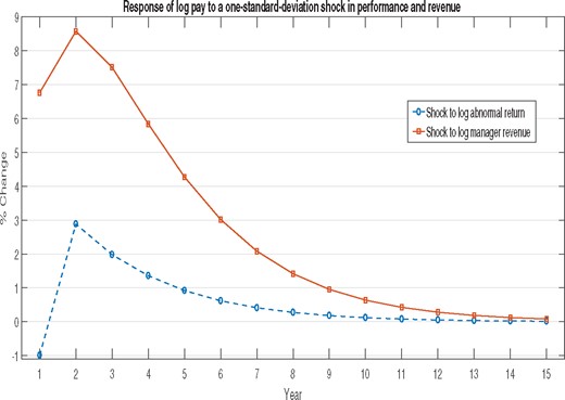
Dynamic response of managerial pay to performance and revenue shocks
The graph shows the response of a mutual fund manager’s labor income to a one-standard-deviation shock to manager-level log abnormal return (dashed line) and to a one-standard-deviation shock to log manager revenue (solid line). These responses are generated from a first-order panel VAR that contains log abnormal return, log revenue, and log labor income (in that order). A Cholesky decomposition of the innovation covariance matrix is used for shock identification. The shock to revenue is orthogonal to performance. The panel VAR is estimated on the full sample of 2,871 manager-year observations using the stata command pvar.
D.3.2 VAR with firm-level revenue added.
We augment the VAR with firm-level revenue, estimating a four-dimensional VAR(1) with the ordering: log abnormal return, log manager-level revenue, log firm-level revenue, and log pay. Figure D2 compares the response of pay to the abnormal return shock, the manager-level revenue shock orthogonalized to abnormal return, and the firm-level revenue shock orthogonalized to both abnormal return and manager-level revenue. A shock to firm-level revenue that is orthogonal to manager-level returns and manager-level revenue exerts an independent effect on managerial pay, after accounting for all the dynamics. The response to this orthogonal firm-level revenue shock is two-thirds that of the manager-level shock and at least as persistent.
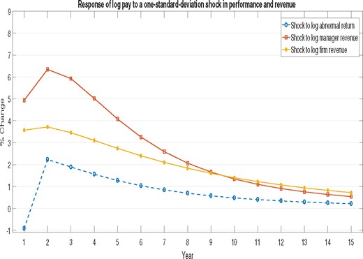
Dynamic response of managerial pay to performance, manager revenue, and firm revenue shocks
The graph shows the response of a mutual fund manager’s labor income to a one-standard-deviation shock to manager-level log abnormal return (dashed line), a one-standard-deviation shock to log manager revenue (solid line with squares), and to a one-standard-deviation shock to log firm revenue (solid line with crosses). These responses are generated from a first-order panel VAR that contains log abnormal return, log manager revenue, log firm revenue, and log labor income (in that order). A Cholesky decomposition of the innovation covariance matrix is used for shock identification. The shock to manager revenue is orthogonal to performance. The shock to firm revenue is orthogonal to performance and manager revenue. The panel VAR is estimated on the full sample of 2,871 manager-year observations using the stata command pvar.
Appendix E. Assignment Model and the Managerial Talent Distribution
Equation (E1) implies that the elasticity of wages to revenue at the median firm is given by |$e+f=\gamma$|. If |$\gamma=1$|, a doubling in the revenue at the median firm doubles median manager compensation. This equation holds for large mutual funds, that is, the right tail of the mutual fund manager revenue distribution. We estimate it by selecting the largest 25% (left panel of Table E1) or the largest 50% (right panel) of managers by revenue in each year. The intercept |$d$| depends on the investment category or manager if the performance impact of talent depends on the category or manager. We explore one specification where |$d$| is constant, one where |$d$| depends on the investment category and where we simultaneously include our other controls, and one where we add manager fixed effects so that |$d$| becomes manager-specific. Following Gabaix and Landier (2008), we omit year fixed effects and report standard errors clustered both at the manager level (first line) and at the year level (second line).
Pay in the tail of the size distribution
| (1) | (2) | (3) | (4) | (5) | (6) | |
|---|---|---|---|---|---|---|
| |$\log (L_{\it m,t})$| | |$\log (L_{\it m,t})$| | |$\log (L_{\it m,t})$| | |$\log (L_{\it m,t})$| | |$\log (L_{\it m,t})$| | |$\log (L_{\it m,t})$| | |
| |$ \log ({\it REV}_{\it m,t})$| | 0.126* | 0.0997 | 0.217*** | 0.160*** | 0.118*** | 0.168*** |
| (0.0714) | (0.0801) | (0.0703) | (0.0376) | (0.0442) | (0.0484) | |
| (0.0397) | (0.0431) | (0.0472) | (0.0185) | (0.0206) | (0.0299) | |
| |$\log({\it REV}_{{\it f,t,median,}25})$| | 0.0842 | 0.0628 | 0.0210 | |||
| (0.107) | (0.105) | (0.0728) | ||||
| (0.0838) | (0.0636) | (0.0724) | ||||
| |$\log({\it REV}_{{\it f,t,median,}50})$| | 0.0784 | 0.0306 | –0.0152 | |||
| (0.0498) | (0.0506) | (0.0395) | ||||
| (0.0638) | (0.0434) | (0.0585) | ||||
| Constant | 10.29*** | 5.611** | 1.645 | 9.810*** | 6.004*** | 6.083*** |
| (1.641) | (2.576) | (4.398) | (0.986) | (1.385) | (2.171) | |
| (1.265) | (1.299) | (2.763) | (1.085) | (0.862) | (1.588) | |
| Manager FE | No | No | Yes | No | No | Yes |
| Year FE | No | No | No | No | No | No |
| Category FE | No | Yes | Yes | No | Yes | Yes |
| Controls | No | Yes | Yes | No | Yes | Yes |
| |$N$| | 922 | 803 | 803 | 1,848 | 1,607 | 1,607 |
| Adjusted |$R^{2}$| | 0.013 | 0.164 | 0.700 | 0.044 | 0.179 | 0.671 |
Panel regression of log manager labor income on a constant, log manager revenue, and log median revenue. The first set of standard errors is clustered at the manager level, the second set is clustered at the year level. The first three columns select the top 25% of observations each year based on manager revenue. The last three columns select the top 50% of observations each year based on manager revenue. The median revenue we use is taken among the firms that employ the managers in the included part of the manager revenue distribution (top 25% or top 50%).
Table E1 finds an estimate of 0.084 for |$e$| and 0.126 for |$f$| for the top 25% managers in terms of manager-level revenue (Column 1). The estimates for the top 50% of managers in Column (4) are similar: 0.078 for |$e$| and 0.160 for |$f$|. The estimates for |$f$| are similar to the 0.14–0.15 point estimate we obtained for the full sample of managers in Table 2. This confirms our earlier observation that a linear relationship between log labor income and log revenue fits the data well (recall Figure 3), across the entire revenue distribution.
Columns (1) and (4) imply a similar point estimate for the elasticity of managerial impact |$\gamma=e+f$| around 0.22. All columns of Table E1 imply values between 0.15 and 0.25. An alternative way of estimating |$\gamma$| is from a time-series regression of log median wages on log median revenue, where the median is within the subset of highest revenue managers. We find a value of 0.57 with standard error 0.12.43 The 0.15–0.57 value range for |$\gamma$| estimated from Swedish mutual fund managers is far below the value of 1 Gabaix and Landier (2008) estimate for U.S. CEOs. It implies strongly decreasing returns to scale from having more talented managers run larger mutual funds, in terms of the additional revenues they generate, compared with constant returns to scale found for CEOs.
We find a value of |$\alpha = 1.11$| with a standard error of 0.045, clustered at the manager level. In other words, the revenue distribution is similarly fat-tailed to the U.S. firm size distribution.
With this estimate for |$\alpha$| in hand, the estimates for |$e$| in Columns (1) and (4) imply |$\beta$| estimates below 0.1. These estimates suggest a much more thin-tailed talent distribution for Swedish mutual fund managers than for U.S. CEOs, where the implied |$\beta=2/3$|.
In sum, compared with U.S. CEOs where there is constant returns to scale from having more talented CEOs run larger firms, we find strongly decreasing returns to scale from having more talented managers run larger funds. This suggests that returns to scale from managerial talent are different for mutual funds compared with other corporations. We also find that the talent distribution of Swedish fund managers is not as fat-tailed as that of U.S. corporate CEOs. This could be attributed to a couple of potential factors. First, the talent distributions could inherently differ across different institution types. Second, the Swedish economy is considerably smaller than the U.S. economy, so even when we focus on the largest 100 funds in comparison to the largest 500 U.S. corporations we may not be comparing equivalent segments of the tail. Disentangling the two possibilities is an interesting question for future research.
Appendix F. Partnership Income
F.1. Ownership data
Recall that we already included dividend income in a more comprehensive measure of income in Section 4.2. This includes dividend income in own-company stock. However, all other sources of partnership income a manager may receive are not included in this measure. However, it is possible to measure partnership income reasonably well. If the manager receives partnership income as an individual, we can obtain that information from the K-10 tax form available through Statistics Sweden. If the manager sets up a limited liability company, or a chain of limited liability companies, to receive the partnership income, we can combine information from the K-10 tax form with the firm-level database Serrano to unravel the ownership stakes.
We are able to identify ownership stakes in fund companies with two caveats. First, we are only able to do so after 2005 since that is the starting date of the K-10 data. Second, in case a manager holds a stake in a fund company via a limited liability company, we are able to identify the ownership stake only if the ownership stake is larger than 20%. Ownership stakes between companies that are less than 20% are not reported in the Serrano database. Ownership stakes of persons (as opposed to LLCs) are not subject to this truncation.
We identify 225 of the 2,419 manager-year observations and 51 of the corresponding 498 managers as managers who own a stake in one of our fund companies post-2005. Of the 225 manager-year observations, 72 report a direct (personal) ownership in the fund company, 103 report ownership in a firm that in turn reports ownership in one of our fund companies, 47 observations involve an ownership chain with two firms, and 3 observations report ownership with three firms in the chain. When the ownership occurs through a LLC or a chain of LLCs, we multiply the ownership stakes between these companies to arrive at the final ownership stake in the fund company. The distribution of the final ownership stake for the 225 observations looks as follows: 25th percentile is 5%, 50th percentile is 34%, 75th percentile is 50%, and the 90th percentile is 75%.
As noted above, the ownership link between a firm and the manager is not reported in Serrano if the stake is less than 20%. We have done additional work to assess how serious the 20% truncation for fund company stakes is. To that end, we have looked at all firms that satisfy the following five criteria: (i) the manager is on the board of the limited liability firm, (ii) he/she is the CEO, (iii) the firm has zero employees, (iv) the number of board members is less than eight, and (v) the industry classification of the firm is “Finance & Real Estate,” “IT & Electronics,” “Corporate Services,” or missing. The resulting list of candidate firms contains 2,705 firms. We then download the annual reports for these firms and individually check the stated purpose of the firm. Many of these candidate firms are completely unrelated to the fund management industry. In case a firm is indeed a limited liability company that owns a stake in a fund company, it lists the name of the fund company it holds shares in and often the number of shares held and the %-stake for a given year. We are able to link 52 firms (corresponding to 43 managers) to fund companies in our sample. Many of these are already in the results discussed above because the ownership stake of the limited liability firm in the fund company is larger than 20%. Only 14 firms (corresponding to 12 managers) report an ownership stake that is less than 20%. We conclude that the truncation at the 20% threshold is not a threat to our results.
F.1.1 Ownership income.
To obtain a measure of income from partnership stakes, we multiply the ownership stake in the fund company with the profit of that fund company. We lose 10 observations due to negative profit, resulting in a sample of 2,409 manager-year observations.
To check that our results are robust to the inclusion of partnership income, we add partnership income to our labor income measure and rerun our main results table. The results are in Table F1. Column (1) reports the pay-revenue elasticity in our baseline specification with controls when manager pay excludes partnership income, but for the post-2005 sample of 2,409 manager-year observations. Column (3) does the same for the pay-performance elasticity, and Column (5) has both revenue and performance on the right-hand side. Columns (2), (4), and (6) have log partnership plus labor income as the left-hand side variable. Comparing Columns (1) and (2), we find a minor increase in the pay-revenue sensitivity from 0.151 to 0.157 when including partnership income. We also see a minor increase in the pay-performance sensitivity from 0.632 to 0.726. We conclude that our results are robust to this addition.
Including partnership income
| (1) | (2) | (3) | (4) | (5) | (6) | |
|---|---|---|---|---|---|---|
| |$\log (L_{\it m,t} + {\%}_{\it m,f,t} \times$| | |$\log (L_{\it m,t} + \%_{\it m,f,t} \times$| | |$\log (L_{\it m,t} + \%_{\it m,f,t} \times$| | ||||
| |$\log (L_{\it m,t})$| | |${\it PROFIT}_{\it f,t})$| | |$\log (L_{\it m,t})$| | |${\it PROFIT}_{\it f,t})$| | |$\log (L_{\it m,t})$| | |${\it PROFIT}_{\it f,t})$| | |
| |$\log ({\it REV}_{\it m,t})$| | 0.151*** | 0.157*** | 0.149*** | 0.155*** | ||
| (0.0215) | (0.0242) | (0.0215) | (0.0242) | |||
| |$\log(1+R^{\it abn}_{{\it m,t-}1})$| | 0.632*** | 0.726*** | 0.372* | 0.455* | ||
| (0.231) | (0.263) | (0.218) | (0.255) | |||
| Constant | 7.240*** | 5.972*** | 9.670*** | 8.507*** | 7.280*** | 6.020*** |
| (0.644) | (0.974) | (0.651) | (0.969) | (0.647) | (0.977) | |
| Manager FE | No | No | No | No | No | No |
| Year FE | Yes | Yes | Yes | Yes | Yes | Yes |
| Category FE | Yes | Yes | Yes | Yes | Yes | Yes |
| Controls | Yes | Yes | Yes | Yes | Yes | Yes |
| |$N$| | 2,409 | 2,409 | 2,409 | 2,409 | 2,409 | 2,409 |
| Adjusted |$R^{2}$| | 0.241 | 0.197 | 0.150 | 0.129 | 0.242 | 0.198 |
Appendix G. Alternative Performance Measures
So far, we used a simple metric of performance, the gross abnormal return, to assess the effect of outperformance on compensation. Table G1, Column (1), repeats the results for our main specification. The other columns show that this result is robust to eight alternative performance measures. Every specification includes manager revenue, controls, and year and category fixed effects. Column (2) uses the gross fund return in excess of the risk-free rate, a more naive outperformance measure. The point estimate is essentially zero. Column (3) uses the gross abnormal return obtained from the capital asset pricing model. The PPS coefficient is zero. The same is true for the Fama-French abnormal return in Column (4), where the factors additionally include the Swedish SMB and HML factors. In Column (5) we use the global five-factor model alpha to measure outperformance. A positive five-factor alpha does not seem related with higher pay.
Alternative performance
| (1) | (2) | (3) | (4) | (5) | (6) | (7) | (8) | (9) | |
|---|---|---|---|---|---|---|---|---|---|
| |$\log (L_{\it m,t})$| | |$\log (L_{\it m,t})$| | |$\log (L_{\it m,t})$| | |$\log (L_{\it m,t})$| | |$\log (L_{\it m,t})$| | |$\log (L_{\it m,t})$| | |$\log (L_{\it m,t})$| | |$\log (L_{\it m,t})$| | |$\log (L_{\it m,t})$| | |
| |$\log ({\it REV}_{\it m,t})$| | 0.140*** | 0.141*** | 0.140*** | 0.140*** | 0.142*** | 0.139*** | 0.140*** | 0.140*** | 0.140*** |
| (0.0195) | (0.0193) | (0.0196) | (0.0196) | (0.0200) | (0.0191) | (0.0198) | (0.0198) | (0.0194) | |
| |$\log (1+R^{\it abn}_{{\it m,t-}1})$| | 0.148 | ||||||||
| (0.176) | |||||||||
| |$\log (1+ R^{\it exc}_{{\it m,t-}1})$| | –0.0314 | ||||||||
| (0.0840) | |||||||||
| |$\log(1+ R^{\it abn, CAPM}_{{\it m,t-}1})$| | 0.0511 | ||||||||
| (0.125) | |||||||||
| |$\log(1+ R^{{\it abn, FF}3}_{{\it m,t-}1})$| | 0.0727 | ||||||||
| (0.130) | |||||||||
| |$\log (1+ R^{{\it abn, GF}5}_{{\it m,t-}1})$| | –0.0532 | ||||||||
| (0.151) | |||||||||
| |${\it ValueAdded}_{{\it m,t-}1}$| | 0.0486 | ||||||||
| (0.0600) | |||||||||
| |${\it rank}(R^{\it abn}_{{\it m,t-}1})$| within firm | 0.00123 | ||||||||
| (0.00192) | |||||||||
| |${\it rank} (R^{\it abn}_{{\it m,t-}1})_{\it std}$| within firm | 0.000806 | ||||||||
| (0.00192) | |||||||||
| |$\log(1+ R^{\it exc}_{\it m,t-1})$| within category | 0.0703 | ||||||||
| (0.106) | |||||||||
| Constant | 7.212*** | 7.172*** | 7.165*** | 7.174*** | 7.574*** | 7.188*** | 7.185*** | 7.181*** | 7.189*** |
| (0.602) | (0.596) | (0.609) | (0.609) | (0.637) | (0.595) | (0.595) | (0.596) | (0.600) | |
| Manager FE | No | No | No | No | No | No | No | No | No |
| Year FE | Yes | Yes | Yes | Yes | Yes | Yes | Yes | Yes | Yes |
| Category FE | Yes | Yes | Yes | Yes | Yes | Yes | Yes | Yes | Yes |
| Controls | Yes | Yes | Yes | Yes | Yes | Yes | Yes | Yes | Yes |
| |$N$| | 2,898 | 2,898 | 2,885 | 2,885 | 2,795 | 2,898 | 2,898 | 2,898 | 2,898 |
| Adjusted |$R^{2}$| | 0.229 | 0.229 | 0.228 | 0.228 | 0.219 | 0.229 | 0.229 | 0.229 | 0.229 |
See Table 2. Columns (2)–(9) replace our baseline measure of manager abnormal return by manager gross CAPM alpha, gross Fama-French three-factor alpha, gross global five-factor alpha, manager value-added (|$V_{m}$|), the rank of the manager with the firm (worst performing manager receives rank of 1), the rank based on standardized abnormal return, or the gross return of the manager in excess of the average return of all managers in the same investment category.
Column (6) uses gross value added in billions of SEK, the measure advocated by Berk and van Binsbergen (2015). The results are the same as for our main measure of abnormal returns: no PPS to value added beyond the effects on revenue. Replacing gross value added by net value added does not affect this conclusion, since the regression already contains revenue, which is the difference between gross and net value added.
Columns (7)–(9) explore the concept of relative performance evaluation. In Column (7), we rank all managers in the same firm by their gross abnormal return each year. The worst performer receives rank 1, the best one rank |$N$|. The point estimate in Column (7) is positive, as expected, but is not different from zero. The second rank variable in Column (8) uses a standardized performance measure instead, with a cross-sectional mean of 0 per category and year and scaled by the standard deviation of the category. Again, the point estimate is not different from zero. Finally, Column (9) uses the return of the manager in excess of the average return of all managers in the same investment category as the performance measure. The point estimate is similar to that in Column (1) and remains insignificant. In unreported results, we also considered nonlinear specifications for the different performance measures, with similar results.
The evidence suggests that firms do not seem to use sophisticated factor models to asses performance in their determination of managerial compensation. The simplest performance measure, benchmark-adjusted returns, works the best. This echoes the results of Berk and van Binsbergen (2016) on the investors’ use of simple models of performance in the determination of fund flows.
References
Footnotes
1Bodnaruk and Simonov (2015) collect similar data, but study whether Swedish mutual fund managers’ personal portfolio allocations evidence investment acumen. In contemporaneous work, Ben-Naim and Sokolinski (2017) study income data of Israeli mutual fund managers. They confront this data with a model that extends Gennaioli, Shleifer, and Vishny (2015). Mutual fund managers contribute familiarity, which attracts fund flows and increases the pay-performance sensitivity.
2 A small fraction of funds have a performance fee component; 10% in the United States (Elton, Gruber, and Blake 2003). When present, it is typically symmetric per the 1970 amendment to the Investment Advisors Act of 1940. In some cases the rate is fixed up to a given level, with net assets above that level receiving lower marginal rates. Concavity is lower for smaller funds and funds that are part of smaller fund families (Deli 2002). Coles, Suay, and Woodbury (2000) and Deli (2002) examine how cross-sectional variation in fees is determined by fund characteristics, and Warner and Wu (2011) study fee changes.
3 A large theoretical literature studies which contracts should emerge under delegation. While earlier work argues for the suboptimality of linear performance fees in static settings (Admati and Pfleiderer 1997; Stoughton 1993), later work rationalizes performance based compensation and benchmarking in a variety of settings (Basak and Pavlova 2013; Buffa, Vayanos, and Wooley 2014; Cuoco and Kaniel 2011; Heinkel and Stoughton 1994; Li and Tiwari 2009; Ou-Yang 2003).
4 Using U.S. data from the Statement of Additional Information, Ma, Tang, and Gomez (2016) document that 79% of funds have compensation contracts feature a bonus contingent on performance. This data speaks to the nature but not the strength of performance-based pay. Ma, Tang, and Gomez (2016) also document the prevalence of longer evaluation horizons.
5 In related work, Del Guercio and Reuter (2014) find that retail investors who prefer to invest through brokers end up in underperforming funds, presumably because of agency conflicts between investors and brokers. Egan (2017) and Roussanov, Ruan, and Wei (2017) develop broker-intermediated demand models for convertible bonds and mutual funds, respectively. We find evidence of weaker incentive-based pay for managers in the mutual fund arms of the four large Swedish retail banks.
6Gervais, Lynch, and Musto (2006) show theoretically that a large fund family’s firing decisions help increase credibility of its retained managers. Some decisions are made exclusively at the family level, such as which funds to advertise (Gallaher, Kaniel, and Starks 2006), incubation strategies (Evans 2010), and determination of number and type of funds as well as whether to allow free switching within funds of the family (Massa 2003). Gaspar, Massa, and Matos (2006) show that fund families strategically shift performance between funds. Bhattacharya, Lee, and Pool (2013) show that affiliated funds provide an insurance pool against temporary liquidity shocks that hit a mutual fund. Sialm and Tham (2016) find that flows to mutual funds also depend on the prior performance of the funds’ management companies. Berk, van Binsbergen, and Liu (2017) show that fund owners have insight into the talent of their managers and reward the best ones with larger funds to manage.
7 For instance, the Swedish bank Handelsbanken operates as “Handelsbanken Rahastoyhtiö Oy” in Finland, as “Handelsbanken Kapitalforvaltning AS” in Norway, and as “Handelsbanken Fonder AB” in Sweden. We keep track of these three separate fund companies since they are separate legal entities. In the Swedish accounting database Serrano, we can obtain accounting variables for the Swedish fund company.
8 Given that this field has a fixed character length, the seventh person’s name is often truncated beyond recognition. On a few occasions, but rarely, does this happen to the sixth name. At one point in time, there can be more than one manager managing the fund. Morningstar does not indicate any hierarchy between the managers who manage a fund at the same time. Some of the spells are blank or indicate “team management.” We lose less than 300 spells due to blanks and team management.
9 The most common equity categories are: Other Europe Equity (specializing in Swedish, Norwegian, Finnish, all Nordic stocks, or Russian stocks), Global Equity, Europe Equity, and Emerging Markets Equity. Among fixed-income funds, the most common are Other Europe Fixed Income (specializing in Swedish bonds), Other Fixed Income, and Euro Fixed Income.
10 We annualize by multiplying the monthly average from the available months by 12.
11 AUM values that are missing in the middle of a fund’s AUM time series are imputed using the fund’s return and average net flow rate during the missing period. Missing AUM data points at beginning or end of the time series are not imputed. 69% of our AUM data points are from Morningstar Direct, 2% are from Bloomberg, 2% from hand collection, and 27% are from imputations. Appendix A.2 provides the details of the imputation procedure.
12 In those cases, we use the Morningstar variable “Category”, assigning the most common benchmark for that category to the remaining funds. When the benchmark is a linear combination of indices, and we lack return information some of the component indices, we assign an alternative only to that component, keeping the other components and the index weighting.
13 Betas are estimated using the full sample. The regression includes a constant. We require at least 24 months of data to estimate the beta. Results using rolling beta estimates are similar.
14 Specifically, (i) the Swedish stock market index return (SIXPRX) in excess of the one-month STIBOR rate, (ii) the global equity index (MSCI) in excess of the one-month U.S. Treasury bill rate, (iii) the North American equity index (MSCI) in excess of the one-month U.S. Treasury bill rate, (iv) the European equity index (MSCI) in excess of the one-month EURIBOR rate, and (v) the Asia ex-Japan equity index (MSCI) in excess of the BOJ basic discount rate.
15 Specifically, (i) the Swedish government bond index return (OMRX) in excess of the one-month STIBOR rate, (ii) the global bond aggregate index (Barclays) in excess of the one-month U.S. Treasury bill rate, (iii) the U.S. bond aggregate index (Barclays) in excess of the one-month U.S. T-bill rate, (iv) the euro bond aggregate index (Barclays) in excess of the one-month EURIBOR rate, and (v) the Asian Pacific bond aggregate index (Barclays) in excess of the BOJ discount rate.
16 Equation (9) uses last period’s AUM to compute a manager’s abnormal returns. This ignores the fact that the set of funds a manager manages in month |$t$| may not be the same as in month |$t-1$| and also that the number of managers running a given fund may change between |$t-1$| and |$t$|. Using time-|$t$| weights may cause the opposite problem. Our approach follows Berk, van Binsbergen, and Liu (2017).
17 A fund-year observation is included in this table if at least one manager in our sample manages that fund in that year. We note that our sample has more funds than managers. Before any filters are applied, the raw data contain 1,600 funds and 1,324 managers. This is because the Morningstar manager field is missing for quite a few funds, and for others there is the useless manager name value “Team Management.” Our need to know the manager’s identity (so as to identify her pay) further increases the ratio of funds to managers. For every manager we can identify, we include all of her funds. We do not require the identity of all other team managers (if team managed) for those funds to remain in the sample. Our average number of funds per manager is similar to the U.S. data. For 2011, Berk, van Binsbergen, and Liu (2017) report 2.47 funds per manager. In that same year, our Swedish data has 2.44. Our sample has fewer managers per fund (1.46) compared with the United States (2.84), which helps to explain why the U.S. data has more managers than funds.
18 The labor income tax rate is 30% up to 439,000 SEK, 50% for additional income between 439,000 and 638,000 SEK, and 55% for income above 639,000 SEK. The dividend income tax rate is 30%.
19 The dividend income likely reflects ownership in the mutual fund company. We investigate income derived from partnership stakes in more detail in Section 4.2.
20 The Serrano data coverage starts in 1998.
21 Specifications that contain lagged revenue result in nearly identical pay-revenue sensitivities.
22 Results are similar when controls are measured contemporaneously with pay.
23 In each category, we pool the observations from all years. We do not have enough observations to calculate standard deviations for each year separately. However, we demean all revenues and abnormal returns by year and category.
24 This is an indicator variable which takes the value of one if an individual’s broad education category is “business administration and trade” and narrow education category is “specialization in banking, insurance and finance.” It is 1 for 59 out of 2,898 manager-year observations.
25Kacperczyk, Van Nieuwerburgh, and Veldkamp (2014, 2015) provide a model and empirical evidence for time-varying skill among mutual fund managers.
26 In unreported results, we have explored specifications that specify labor income levels and linear and linear-quadratic functions of revenue. Those specifications do not fit the data as well as the log-log specification.
27 For that reason, it is a natural starting point in which to study the relationship between an individual manager’s pay and that manager’s revenue, as in Equation (11). This comparison, however, should not be seen as an endorsement for the Berk and Green model. The evidence in Section 4 strongly suggests that the mutual fund firm is more than a collection of managers each running their own fund, and explores the role of the firm level in determining pay.
28 A similarly poor fit exists with abnormal returns on the x-axis, instead of log abnormal returns.
29 In unreported results, we have added quadratic terms of abnormal returns in the orthogonalization step—to account for a possibly convex flow-performance relationship—but found similar results.
30 By law, firms in the United States have to report one, five and ten years of past performance plus a graph showing performance over ten years. This is confirmed in the Statements of Additional Activity studied by Ma, Tang, and Gomez (2016).
31 The same conclusion can be drawn from the last column of Table 3 when adding the coefficient on the contemporaneous abnormal return.
32 In unreported results, we have extended the results to include a fourth lag of performance with similar results. We also exploit the change in performance evaluation horizon that came into effect in 2009 per European mandate. We find somewhat stronger PPS effects in the post-2009 sample than in the full sample. Our conclusions on the quantitative importance of performance-based pay are unaffected, however.
33 The filing by Janus Capital, the employer of Bill Gross, is a good example. It states: “The overall investment team variable compensation pool is funded by an amount equal to a percentage of Janus Capital’s pre-incentive operating income. In determining individual awards, both quantitative and qualitative factors are considered. Such factors include, among other things, consistent short-term and long-term fund performance, client support and investment team support through the sharing of ideas, leadership, development, mentoring, and teamwork.”
34 If a manager works for more than one firm during a given year, we assign him/her to the firm he/she has worked the longest for as of that year. For the 2,898 observations in our baseline regressions, the distribution of the variable “number of firms in a year” is 1 until the 75th percentile, 2 at the 90th and 95th and 3 at the 99th percentile.
35 Because colleagues’ revenue is zero for firms with only one fund, we lose these observations. There is nothing to learn about the role of firm-level variables in one-fund firms.
36 The Big 4 account for 1,109 out of 2,898 manager-year observations, 29.1% of total pay, 46.9% of AUM, and 47% of revenue. These 1,109 observations belong to 241 managers.
37 Average compensation is SEK 1.54 million at the Big 4 compared with SEK 1.57 million elsewhere.
38 Month by month we assign the manager the category of the fund with the highest AUM. The yearly category variable is the most prevalent monthly assigned category. To ensure sufficient observations, quartiles are formed by pooling all years. Results for terciles or quintiles are similar. We also explored (30,40,30), (20,60,20), and (10, 80, 10) groupings with consistent results.
39 See the last two columns of Table B2 in Appendix B.
40Board equals 1 not only if a manager is on the board of one of the firms he works for but also if he is on the board of a holding company that has shares in the firm that manages the funds. There are 691 manager-year observations in Columns (7)–(9) for whom Board equals 1, or 23.8% of the sample.
41 In the extended sample with the exit year, about 7.5% of observations are such exits (245 observations out of 3,263).
42 Implicit is the approximation that |$\log\left(\frac{{\it AUM}_{\it it}}{{\it AUM}_{it-1}}\right) \approx \frac{{\it AUM}_{\it it}}{{\it AUM}_{it-1}}-1$|.
43 The slope of this time-series regression is sensitive to the sample used. If we start the sample after 1995, the point estimate drops to 0.45 (0.06) and if we start the sample only in 2000, it drops to 0.14 (0.08). Visual inspection confirms that median compensation and median revenue were both growing in tandem in the years before 2000. After 2000, median wages started to grow much slower than median manager revenue.
