


Abstract
This paper identifies a new channel through which bankrupt firms undergoing liquidation impose negative externalities on their nonbankrupt peers. The liquidation of a retail chain weakens the economies of agglomeration in any given local area, reducing the attractiveness of retail centers for remaining stores and leading to contagion of financial distress. We find that firms with greater geographic exposure to bankrupt retailers are more likely to close stores in affected areas. We further show that the effect of these externalities on nonbankrupt peers is higher when affected stores are smaller and are operated by firms in financial distress.
Received December 16, 2015; editorial decision June 28, 2018 by Editor Philip Strahan.
How do bankruptcy, liquidation, and financial distress spread? Research on bankruptcy and financial distress has documented how bankruptcy reorganizations affect firms that file for Chapter 11 themselves (e.g., Asquith, Gertner, and Scharfstein 1994; Hotchkiss 1995; Stromberg 2000). However, evidence on the effect of bankruptcy, liquidations, and financial distress on competitors and industry peers is limited. In this paper, we identify a new channel by which bankrupt firms undergoing liquidation impose negative externalities on their nonbankrupt competitors, namely, through their impact on the sales of peer firms and on their propensity to close stores.
Research in industrial organization has argued that the geographic concentration of stores and the existence of clusters of stores can be explained by consumers’ imperfect information and their need to search the market (Wolinsky 1983). Indeed, both practitioners and academics argue that economies of agglomeration exist in retail since some stores—those of national name-brands or anchor department stores, in particular—draw customer traffic not only to their own stores but also to nearby stores. As a result, store-level sales may depend on the sales of neighboring stores for reasons that are unrelated to local economic conditions (Gould and Pashigian 1998; Gould, Pashigian, and Prendergast 2005).
We conjecture that the externalities that exist between neighboring stores, and the economies of agglomeration they create, can be detrimental during downturns, propagating and amplifying financial distress and liquidations among firms operating in the same locality. Our main hypothesis is that retail store closures—because of firm-wide liquidation or as a result of a bankruptcy reorganization—imposes negative externalities on neighboring firm stores. The reduction in agglomeration economies reduces the economic value of neighboring stores, reducing their sales and increasing their likelihood of closure. If such negative externalities are sufficiently strong, the liquidation of a given firm’s stores will propagate within a given area, reducing the economic value of nearby stores and ultimately increasing the likelihood of further liquidations. In the extreme, beyond closing individual stores, firms experiencing neighboring store closures may be pushed into bankruptcy themselves, which may result in partial or even full liquidation of the firm’s stores.
Theoretically, diseconomies of agglomeration do not require store liquidations. Financial distress at the parent level, say in bankruptcy reorganization, may adversely affect store attractiveness and costumer traffic (e.g., because of a reduction in advertising or store-specific factors, such as inventory levels), which, in turn, impose negative externalities on neighboring stores. However, our identification strategy exploits Chapter 11 bankruptcies and liquidations of national retailers that liquidate their entire store chain. We do this for two reasons. First, as explained below, this strategy of using national bankruptcies is employed to identify the causal effect of store closures that are unrelated to local economic conditions. Second, our empirical strategy also provides an important conceptual contribution, namely, a novel amplification and propagation mechanism by which firms undergoing liquidation (as a result of financial or economic distress) cause further distress in firms owning neighboring stores, thereby leading to further store closures.
This result relates directly to an important question in the literature on restructuring and reorganization relating to the costs of liquidation outcomes in bankruptcy. One view is that liquidation is efficient since assets go to the best user (see, e.g., Baird 1986). The other view is that liquidation may not lead to efficient outcomes, as the first best user may be financially constrained and hence lose the auction in liquidation (Shleifer and Vishny 1992). By studying the negative externalities stemming from liquidations that lead to the destruction of agglomeration economies we point to an additional factor that should be taken into account in the reorganization versus liquidation debate. More broadly, our paper sheds light on the externalities that bankrupt firms impose on each other, and such externalities are of a particular concern, as they may give rise to self-reinforcing feedback loops that could amplify the business cycle during industry downturns.
Identifying a causal link, however, from the financial distress and liquidation of one retailer to the sales and closure decisions of its neighboring retailers is made difficult by the fact that financial distress and liquidations are correlated with local economic conditions. Correlation in sales among stores in the same vicinity may therefore simply reflect weak demand in an area. Similarly, the fact that store closures tend to cluster locally may often be the outcome of underlying difficulties in the local economy, rather than the effect of negative externalities among stores. Local economic conditions will naturally drive a correlation in outcomes among stores located in the same area.
Using a novel and detailed data set of all national chain store locations and closures across the United States from 2005 to 2010, we provide empirical evidence that supports the view that bankruptcies of retail companies impose negative externalities on neighboring stores owned by solvent companies. Our identification strategy consists of analyzing the effect of Chapter 11 bankruptcies of large national retailers, such as Circuit City and Linens ’N Things, that liquidate their entire store chain.1 Using Chapter 11 bankruptcies of national retailers that liquidated their entire store portfolio alleviates the concern that local economic conditions led to the demise of the company: it is unlikely that a large retail chain will suffer major financial difficulties because of a highly localized economic downturn in one of its many locations. Indeed, all of our results continue to hold even after we control for ZIP-code-by-year fixed effects, thereby controlling for unobserved time-varying heterogeneity at a fine geographical level. Further supporting our identification assumption, we show that stores of retail chains that eventually file for Chapter 11 bankruptcy are not located in areas that are worse than the location of stores operated by chains that avoid bankruptcy, along a host of economic characteristics.2
We show that stores located in proximity to stores of national chains that are liquidated are more likely to close themselves. Importantly, we find that this effect is stronger for stores in the same industry of the liquidating national chain as compared to stores in industries different from that of the liquidating chain. For example, focusing on stores located at the same address (usually mall locations), the probability that a store will close in the year following the closure of a store belonging to a liquidating national chain is approximately two times larger when operating in the same industry as compared to when the stores operate in different industries. That the negative externality is stronger among stores in the same industry is consistent with research in urban economics analyzing economies of agglomeration due to industrial clusters, for example, because of search frictions like in Wolinsky (1983) and Ellison and Glaeser (1997).
We proceed by analyzing additional heterogeneity in the geographical effect of store closures. First, we examine how the negative externality of store closures interact with the financial health of solvent owners of neighboring stores. We hypothesize that the impact of national chain store liquidations will be stronger on firms in weaker financial health: external finance is plausibly more costly and more difficult to obtain for financially weaker firms, and so it is more difficult for them to smooth the economic shock stemming from the negative externality caused by neighboring store closures. Instead, they downsize by closing affected stores. Focusing on stores owned by a parent company, and measuring financial health using the profitability of the parent, we find that, consistent with our hypothesis, the geographical effect of store closures on neighboring stores is indeed more pronounced in financially weaker firms. For example, when located within a 50-m radius of a closing national chain store, stores belonging to parent firms in the 25th percentile of profitability are between 16.9% and 22.2% more likely to close. In contrast, if the parent firm is in the 75th percentile of profitability, there is no statistically significant effect on the likelihood of store closure.
We continue by analyzing how the negative externality of store closers vary by store size. We hypothesize that larger stores should be more resilient to the closure of neighboring stores. This is because larger stores may be less reliant on neighboring stores to generate customer traffic or because larger stores are more profitable, implying that the negative shock does not push them toward economic distress. Consistent with our hypothesis, we find that larger stores do indeed exhibit a lower likelihood of closure following the liquidation of neighboring stores.
In addition, we examine how local economic conditions affect the negative externality of store closures. We find that in lower-income ZIP codes, stores are more likely to close with the exogenous closure of their neighboring stores. Still, the negative externality of store closures appears for the vast majority of ZIP code income levels. Similar to the results based on firm-level profitability, we hypothesize that in low-income areas, stores are less able to smooth the negative externality shock stemming from neighboring store closures. Alternatively, stores in low-income areas may be closer to economic nonviability, and so are more likely to close once diseconomies of agglomeration occur.
Finally, we compare the negative externality of store closures during the financial crisis period of 2008–2009, to the precrisis period of 2006–2007, showing that diseconomies of agglomeration occur outside the crisis as well. Of course, since store liquidations are more prevalent in downturns, the aggregate impact of the negative externality during these periods is likely to be larger.
Our paper is closely related to a large body of work on agglomeration economies that studies how the proximity of firms and individuals in urban areas increases productivity. Prior work has shown that increases in productivity can arise for a variety of reasons, including reduced transport costs of goods, increased ability of labor specialization, better matching quality of workers to firms, and knowledge spillovers.3 Within the retail sector, agglomeration economies may arise because of the increased productivity stemming from reduced consumer search costs. By utilizing micro-level data on store locations and closures, our paper contributes to this important literature in two ways.
The first contribution is our focus on the way in which liquidations both during and outside of downturns damage economies of agglomeration and the productivity enhancements they create. In contrast, prior work has focused on the creation of agglomeration economies through firm entry and employment decisions (see, e.g., Ellison and Glaeser 1997; Glaeser et al. 1992; Henderson et al. 1995; Rosenthal and Strange 2003). By focusing on downturns, our work shows how agglomeration economies can be understood to propagate liquidations and financial distress. Indeed, firm closures will naturally increase distance between agents in an urban environment, which will tend to reduce the productivity of remaining firms due to diseconomies of agglomeration. To the extent that replacing closed stores with new ones takes time—for example, because of credit constraints during downturns—the reduction in productivity may have long term consequences. In this context, our work stands in contrast to a number of other studies in the finance literature analyzing how firms in bankruptcy or financial distress affect their industry peers (see, e.g., Benmelech and Bergman 2011; Hertzel and Officer 2012; Jorion and Zhang 2007; Lang and Stulz 1992). These studies focus on contagion stemming from other sources of externality, such as changes in the cost of external capital in peer firms, information flows, or increased concentration in the competitive landscape.
The second contribution of the paper is the empirical identification of agglomeration economies. The standard difficulty in identifying agglomeration effects is the endogeneity of firms’ location decisions. Namely, is firm proximity causing high productivity or, alternatively, is the proximity simply a by-product of firms choosing to locate in areas naturally predisposed to high productivity? Employing micro-level data on store locations, we address this endogeneity concern by instrumenting for variation in store location with our large retail-chain liquidation of stores instrument.4 As described above, to the extent that national chain store closures are not driven by highly localized demand-side effects, we can measure the impact of store closures on nearby stores. Agglomeration effects, and the degree to which they attenuate with distance to other stores, are therefore estimated at a micro level.
Our paper also adds to the growing literature in finance on the importance of peer effects and networks for capital structure (Leary and Roberts 2014), acquisitions and managerial compensation (Shue 2013), entrepreneurship (Lerner and Malmendier 2013), and portfolio selection and investment (Cohen, Frazzini, and Malloy 2008). In particular, our paper is closely related to Almazan et al. (2010), who link financial structure to economies of agglomeration. In particular, Almazan et al. (2010) show that firms located in industry clusters are more likely to maintain financial slack in order to facilitate acquisitions within these clusters.
1. Identification Strategy
Our main prediction is that, because of the economics of agglomeration, retail store closures impose negative externalities on their neighbors; that is, store sales tend to decrease with a decline in customer traffic in their area. If this effect is sufficiently large, store closures will tend to propagate geographically. However, identifying a causal link from the financial distress or bankruptcy of retailers to the decision of a neighboring solvent retailer to close its stores is difficult because financial distress is potentially correlated with underlying local economic conditions. For example, that local retailers are in financial distress can convey information about weak local demand. Similarly, that store closures tend to cluster locally does not imply a causal link but rather may simply reflect difficulties in the local economy.
Our identification strategy consists of analyzing the effect of Chapter 11 bankruptcies of large national retailers, such as Circuit City and Linens ’N Things, who liquidated their entire store chain during the sample period. Using Chapter 11 bankruptcies of national retailers alleviates the concern that local economic conditions led to the demise of the company: it is unlikely that a large retail chain will suffer major financial difficulties because of a localized economic downturn in one of its many locations. Still, it is likely that national chains experiencing financial distress will restructure their operations and cherry-pick those stores they would like to remain open. According to this, financially distressed retailers will shut down their worst performing stores while keeping their best stores open, implying that a correlation between closures of stores of bankrupt chains may merely reflect poor local demand rather than negative externalities driven by financial distress. We address this concern directly by only utilizing variation driven by bankruptcy cases that result in the liquidation of the entire chain. In these cases, cherry-picking of the more successful stores is not a concern; all stores are closed regardless of local demand.
In examining national chain liquidations, one concern that remains is that the stores of the liquidating chain were located in areas that experienced negative economic shocks—for example, because of poor store placement decisions made on the part of headquarters—and that it was these shocks that eventually drove the chain into bankruptcy. We address this concern in two ways. First, based on observables, we empirically show that stores of chains that eventually file for Chapter 11 bankruptcy and fully liquidate are not located in areas that are worse than the location of stores operated by chains that avoid bankruptcy. Second, because of our precise data on the location of each store and our use of area fixed effects (county, ZIP code, or ZIP-code-by-year), our identification strategy enables us to net out local economic shocks and relies on variation within the relevant geographic area. As such, the relevant endogeneity concern is not that the stores of liquidating national chains were located in areas that suffered more negative economic shocks, but rather that these stores were somehow positioned in the worse locations within each county or ZIP code. Given their firms’ success in forming a national chain of stores, this seems highly unlikely.
To further alleviate concerns about store locations, we also perform a placebo test. We define a “placebo” variable that counts for each store in our sample the number of neighboring stores that are part of a national chain that will liquidate in the following year but that are currently not in bankruptcy. We find that the effect of store liquidation on subsequent store closures is not driven by the location of the retail chain-stores that will later become bankrupt but rather by the timing in which they were actually closed. This effect is consistent with the existence of a causal effect of store closures.
2. Data and Summary Statistics
2.1 Sample construction and data sources
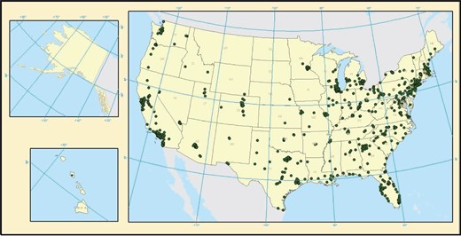
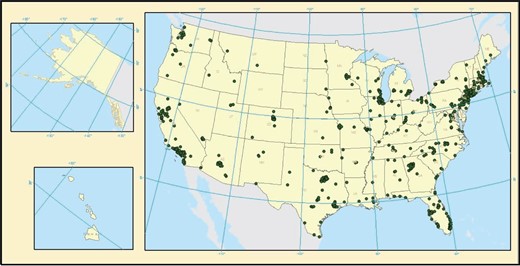
Our data set comprises several sources, which we describe in this section. The main source is Chain Store Guide (CSG), a database that contains detailed information on retail store locations in the United States and Canada. CSG data are organized in the form of annual snapshots of almost the entire retail industry at the establishment level.5 The information on each location contains the store name, its address (street number, street name, city, state, and ZIP code) and phone number, the parent company, and a CSG-defined industry.6 Our sample covers the 2005–2010 period and includes 828,792 store-year observations in the United States in the following CSG-defined industries: Apparel Stores, Department Store, Discount Stores, General Merchandise Store, Home Centers & Hardware Chains, and Value-Priced Apparel Store. Figures 1 and 2 demonstrates the coverage of our data by plotting the locations of all stores in our data set for the first year (2005 in Figure 1) and the last year of our sample (2010 in Figure 2).
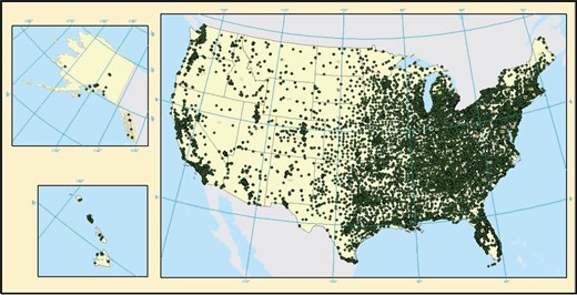
Store locations as of 2005
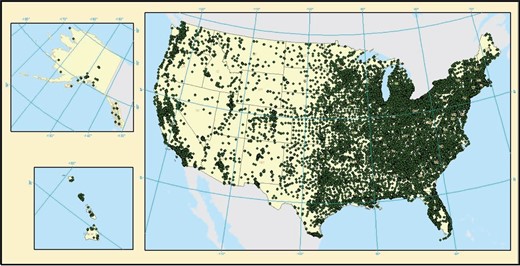
Store locations as of 2010
We clean the data and streamline store names and parent names for consistency. Large chain stores account for the bulk of the data. For example, in 2010, the 50 largest retail chains accounted for 111,655 of the 166,045 stores in the data set, representing 67.2% of the stores in the data for that year.
Our empirical strategy requires us to compute distances between retail locations. To do so, we convert all street addresses into geographic coordinates using ArcGIS software. If an address is not contained in the address locator used by ArcGIS, we pass it through Google Maps API in an additional attempt to geocode it. As a result, we successfully map street addresses to geographic coordinates for 97% of the data. The information on longitudes and latitudes of full addresses—up to a street number—makes it possible for us to compute distances between retail locations to a very high precision. Since our analysis focuses on stores that are in close proximity to each other, we use the standard formula for the shortest distance between two points on a sphere (see Coval and Moskowitz 1999) without adjusting for the fact that the Earth’s surface is geoid shaped.
We supplement the CSG store-level data with information on the number of employees and store selling area size from Esri’s Business Analyst. Esri’s data structure is very similar to that of CSG. We carefully merge these two databases by store/parent name and address; questionable cases are checked manually. The majority of information on the number of employees available is collected by Esri by reaching out individually to every store on a yearly basis; about 10% of the data though is populated according to the data provider’s proprietary models based on observable characteristics of a retail location. In our analysis, we use only the actual data points and discard modeled figures.
We also use Esri’s Major Shopping Centers, which is a panel of major U.S. shopping centers, to group stores in our sample into malls where applicable. The included mall-level pieces of information are mall name and its address (usually up to a street intersection), gross leasable area (GLA), total number of stores, and names of anchor tenants (up to four). We merge Esri’s Major Shopping Centers to CSG data using the following multistep procedure. First, we find anchor stores in the data using the information on store/parent name and ZIP code. If several anchor stores pertaining to the same mall are identified, we confirm the match if the average distance from anchors to the implied center of the mall is less than 200 m. By doing so, we increase our confidence that we do not erroneously label stores as anchor tenants in ZIP codes containing a large number of stores. Stores located within 25 m of anchors are assigned to the same mall. Second, we geocode addresses of malls that were not found in the data using anchor tenants—for example, information about their anchors is missing—to compute distances between malls and stores. All stores within 100 m of the mall are assigned to that mall. At all stages of the algorithm, we manually check questionable cases by looking up store addresses and verifying whether they are part of a shopping mall.
Next, we use SDC Platinum to identify retail Chapter 11 bankruptcies since January 2000 within the following SIC retail trade categories: general merchandise (SIC four-digit codes 5311, 5331, and 5399), apparel (5600, 5621, and 5651), home furnishings (5700, 5712, 5731, 5734, and 5735), and miscellaneous (5900, 5912, 5940, 5944, 5945, 5960, 5961, and 5990). There were 93 cases of retail Chapter 11 liquidations between 2000 and 2011.7 The largest bankruptcies in recent years include Circuit City, Goody’s, G+G Retail, KB Toys, Linens ’N Things, Mervyn’s, and The Sharper Image. Bankrupt stores are identified in our data by their respective parent name.
We then merge our data with Compustat Fundamental and Industry Data. We use the Compustat North America Fundamentals Annual database to construct variables that are based on operational and financial data. These include firm size (defined as the natural log of total assets), market-to-book ratio (defined as the market value of equity and book value of assets less the book value of equity, divided by the book value of assets), profitability (defined as earnings over total assets), and leverage (defined as total current liabilities plus long-term debt, divided by the book value of assets).
We supplement our database with information pertaining to the local economies from the Census, IRS, Zillow, and the BLS. We rely on the 2000 Census survey for a host of demographic variables available by ZIP code. We also use the Internal Revenue Service (IRS) data, which provide the number of filed tax returns (a proxy for the number of households), the number of exemptions (a proxy for the population), adjusted gross income (which includes taxable income from all sources less adjustments, such as IRA deductions, self-employment taxes, health insurance, alimony paid), wage and salary income, dividend income, and interest income at the ZIP code level. We use data on house prices from Zillow, an online real estate database that tracks valuations throughout the United States. We construct annual county-level and ZIP code median house values and annual changes in housing prices.
2.2 Individual store closings
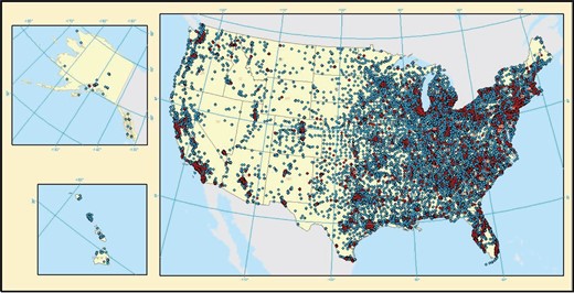
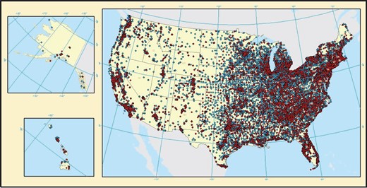
To construct our main dependent variable of store closings, we compare the data from one year to the next. We define a store closure if a store entry appears in a given year, but not in the subsequent one. Given that our data span the years 2005–2010, we can identify store closings for each year from 2005 up to 2009. Panel A of Table 1 provides summary statistics on store closings during our entire sample period and individually for each of the years in the sample. The number of stores in the data ranges from 84,388 individual stores in 2005 to 155,114 stores in 2009. The rate of annual store closure ranges between 1.4% in 2007 to 11.0% in 2008. During the entire sample period of 2005–2009, 6.1% of store-years represent store closures, with a standard deviation of 23.9%. Figures 3 and 4 display the geographical distribution of store closings (dark dots) relative to stores that stay open (light dots) in 2007 and 2008, respectively.
Individual store closings
| A. Closed stores over time | ||||||||
|---|---|---|---|---|---|---|---|---|
| Year | Mean | 25th percentile | Median | 75th percentile | SD | Min | Max | Observations |
| 2005–2009 | 0.061 | 0.0 | 0.0 | 0.0 | 0.239 | 0.0 | 1.0 | 661,382 |
| 2005 | 0.048 | 0.0 | 0.0 | 0.0 | 0.213 | 0.0 | 1.0 | 84,388 |
| 2006 | 0.085 | 0.0 | 0.0 | 0.0 | 0.279 | 0.0 | 1.0 | 125,897 |
| 2007 | 0.014 | 0.0 | 0.0 | 0.0 | 0.116 | 0.0 | 1.0 | 147,551 |
| 2008 | 0.110 | 0.0 | 0.0 | 0.0 | 0.313 | 0.0 | 1.0 | 148,432 |
| 2009 | 0.047 | 0.0 | 0.0 | 0.0 | 0.211 | 0.0 | 1.0 | 155,114 |
| B. Bankrupt stores over time | ||||||||
| Year | Mean | 25th percentile | Median | 75th percentile | SD | Min | Max | Observations |
| 2005–2010 | 0.021 | 0.0 | 0.0 | 0.0 | 0.142 | 0.0 | 1.0 | 827,156 |
| 2005 | 0.010 | 0.0 | 0.0 | 0.0 | 0.100 | 0.0 | 1.0 | 84,388 |
| 2006 | 0.008 | 0.0 | 0.0 | 0.0 | 0.091 | 0.0 | 1.0 | 125,897 |
| 2007 | 0.029 | 0.0 | 0.0 | 0.0 | 0.167 | 0.0 | 1.0 | 147,551 |
| 2008 | 0.042 | 0.0 | 0.0 | 0.0 | 0.201 | 0.0 | 1.0 | 148,432 |
| 2009 | 0.026 | 0.0 | 0.0 | 0.0 | 0.158 | 0.0 | 1.0 | 155,114 |
| 2010 | 0.004 | 0.0 | 0.0 | 0.0 | 0.063 | 0.0 | 1.0 | 165,774 |
| C. Stores closed in full liquidation bankruptcies over time | ||||||||
| Year | Mean | 25th percentile | Median | 75th percentile | SD | Min | Max | Observations |
| 2005–2009 | 0.010 | 0.0 | 0.0 | 0.0 | 0.100 | 0.0 | 1.0 | 661,382 |
| 2005 | 0.002 | 0.0 | 0.0 | 0.0 | 0.049 | 0.0 | 1.0 | 84,388 |
| 2006 | 0.003 | 0.0 | 0.0 | 0.0 | 0.058 | 0.0 | 1.0 | 125,897 |
| 2007 | 0.001 | 0.0 | 0.0 | 0.0 | 0.033 | 0.0 | 1.0 | 147,551 |
| 2008 | 0.0186 | 0.0 | 0.0 | 0.0 | 0.135 | 0.0 | 1.0 | 148,432 |
| 2009 | 0.0193 | 0.0 | 0.0 | 0.0 | 0.137 | 0.0 | 1.0 | 155,114 |
This table provides descriptive statistics on store closings and bankrupt stores. Panel A displays all store closings. Panel B presents bankrupt stores, and panel C presents store closings that result from full liquidation bankruptcies.
Stores closings during 2007
Stores closings during 2008
Panel B of Table 1 provides summary statistics for stores that operated while their company was in a Chapter 11 restructuring. As panel B shows, 2.1% of the 827,156 observations were stores that their companies were operating under Chapter 11 protection. The number of bankrupt stores increased sharply from 4,231 stores in 2007 (representing 2.9% of total stores) to 6,167 bankrupt stores in 2008 (4.2% of total stores). By 2009 many of the bankrupt retailers were liquidated and their stores disappeared resulting in fewer bankrupt stores (3,963 stores representing 2.6% of the stores in our sample). By 2010 most of the remaining bankrupt companies that were not liquidated emerged from Chapter 11 and the number of bankrupt stores fell to 652, or 0.4%, of the stores in our sample.
Finally, we calculate the number of stores that were closed in bankruptcies of chains that were fully liquidated. As we argue previously, these bankruptcy cases are not driven by the specific location of their stores but rather because of a failure of their business plan. Hence, as described in the Identification Strategy section, we use store closures resulting from the chain-wide liquidation of the parent firm to capture the negative externalities of bankruptcy. Panel C of Table 1 displays summary statistics for these chain-wide liquidating stores. The number of stores closed by chains that were fully liquidated in bankruptcy increases from 160 stores in 2007 (0.10% of total stores) to 2,650 (1.86% of total stores) and 2,987 (1.93% of total stores), in 2008 and 2009, respectively.8
2.3 Neighboring store closures
We construct three main measures of neighboring store closures that are driven by liquidation of national retail chains. To do this, for each store in our sample and for every year we measure the distance to any other store in our sample. Specifically, for each store we define its neighboring stores in a series of concentric circles. We consider neighboring stores that are: (1) located at the same address; (2) located at a different address but are within a 50-m radius of the store under consideration; and (3) located at a different address within a radius of more than 50 m but less than or equal to 100 m from the store under consideration.9 In each of these three geographical units, for each store and each year, we then count the number of stores that were closed as a result of a full liquidation of a large retail chain.
Table 2 provides summary statistics for the three measures associated with each of the three geographical units and for counts of neighboring stores outside of the 100-m radius. Panel A of Table 2 displays summary statistics for same address stores that were closed in chain liquidations. From 2005 to 2010, same-address liquidated stores ranged from 0 to 3, with an unconditional mean of 0.028 and a standard deviation of 0.181. For any given store, therefore, the maximum number of stores operating in the same address that were closed as a result of a retail-chain liquidation is three. Panel A also displays the evolution of the same-address measure over time. For example, on average, same-address equals 0 and 0.002 in 2005 and 2006, respectively.10 As the number of bankruptcies rose in 2007 same-address increased to 0.038 in 2007 (range between 0 and 2) and peaked at 0.085 (range between 0 and 3) in 2009.
Neighboring store closures
| A. Same address | ||||||||
|---|---|---|---|---|---|---|---|---|
| Year | Mean | 25th percentile | Median | 75th percentile | SD | Min | Max | Observations |
| 2005–2010 | 0.028 | 0.0 | 0.0 | 0.0 | 0.181 | 0.0 | 3.0 | 827,156 |
| 2005 | 0.0 | 0.0 | 0.0 | 0.0 | 0.0 | 0.0 | 0.0 | 84,388 |
| 2006 | 0.002 | 0.0 | 0.0 | 0.0 | 0.045 | 0.0 | 1.0 | 125,897 |
| 2007 | 0.038 | 0.0 | 0.0 | 0.0 | 0.192 | 0.0 | 2.0 | 147,551 |
| 2008 | 0.016 | 0.0 | 0.0 | 0.0 | 0.127 | 0.0 | 2.0 | 148,432 |
| 2009 | 0.085 | 0.0 | 0.0 | 0.0 | 0.327 | 0.0 | 3.0 | 155,114 |
| 2010 | 0.009 | 0.0 | 0.0 | 0.0 | 0.100 | 0.0 | 2.0 | 165,774 |
| B. Not same address and distance |$\le$| 50 m | ||||||||
| Year | Mean | 25th percentile | Median | 75th percentile | SD | Min | Max | Observations |
| 2005–2010 | 0.012 | 0.0 | 0.0 | 0.0 | 0.115 | 0.0 | 3.0 | 827,156 |
| 2005 | 0.0 | 0.0 | 0.0 | 0.0 | 0.0 | 0.0 | 0.0 | 84,388 |
| 2006 | 0.002 | 0.0 | 0.0 | 0.0 | 0.044 | 0.0 | 1.0 | 125,897 |
| 2007 | 0.009 | 0.0 | 0.0 | 0.0 | 0.099 | 0.0 | 2.0 | 147,551 |
| 2008 | 0.003 | 0.0 | 0.0 | 0.0 | 0.055 | 0.0 | 2.0 | 148,432 |
| 2009 | 0.038 | 0.0 | 0.0 | 0.0 | 0.207 | 0.0 | 3.0 | 155,114 |
| 2010 | 0.010 | 0.0 | 0.0 | 0.0 | 0.111 | 0.0 | 2.0 | 165,774 |
| C. 50 m |$<$| distance |$\le$| 100 m | ||||||||
| Year | Mean | 25th percentile | Median | 75th percentile | SD | Min | Max | Observations |
| 2005–2010 | 0.008 | 0.0 | 0.0 | 0.0 | 0.094 | 0.0 | 3.0 | 827,156 |
| 2005 | 0.0 | 0.0 | 0.0 | 0.0 | 0.0 | 0.0 | 0.0 | 84,388 |
| 2006 | 0.001 | 0.0 | 0.0 | 0.0 | 0.030 | 0.0 | 1.0 | 125,897 |
| 2007 | 0.005 | 0.0 | 0.0 | 0.0 | 0.075 | 0.0 | 2.0 | 147,551 |
| 2008 | 0.002 | 0.0 | 0.0 | 0.0 | 0.044 | 0.0 | 1.0 | 148,432 |
| 2009 | 0.025 | 0.0 | 0.0 | 0.0 | 0.166 | 0.0 | 3.0 | 155,114 |
| 2010 | 0.008 | 0.0 | 0.0 | 0.0 | 0.103 | 0.0 | 2.0 | 165,774 |
| D. Farther from store closures 2005–2010 | ||||||||
| Year | Mean | 25th percentile | Median | 75th percentile | SD | Min | Max | Observations |
| 100–150 m | 0.007 | 0.0 | 0.0 | 0.0 | 0.087 | 0.0 | 3.0 | 827,156 |
| 150–200 m | 0.006 | 0.0 | 0.0 | 0.0 | 0.085 | 0.0 | 3.0 | 827,156 |
| 200–250 m | 0.020 | 0.0 | 0.0 | 0.0 | 0.151 | 0.0 | 4.0 | 827,156 |
| 250–300 m | 0.006 | 0.0 | 0.0 | 0.0 | 0.082 | 0.0 | 3.0 | 827,156 |
| 300–350 m | 0.006 | 0.0 | 0.0 | 0.0 | 0.083 | 0.0 | 4.0 | 827,156 |
| 350–400 m | 0.006 | 0.0 | 0.0 | 0.0 | 0.079 | 0.0 | 3.0 | 827,156 |
| 400–450 m | 0.006 | 0.0 | 0.0 | 0.0 | 0.081 | 0.0 | 3.0 | 827,156 |
| 450–500 m | 0.006 | 0.0 | 0.0 | 0.0 | 0.079 | 0.0 | 4.0 | 827,156 |
This table provides descriptive statistics on full liquidation closings of neighboring stores. Panel A displays store closings in the same address. Panels B and C present store closings for 0- to 50-m and 50- to 100-m distances. Panel D lists summary statistics for distances between 100 and 500 m.
Panels B and C present similar statistics for the 0|$<$|distance|$\le$|50 and the 0|$<$|distance|$\le$|100 measures, respectively. As can be seen, both measures display similar patterns over time ranging from 0 to 3 and averaging approximately 0.01. Finally, panel D expands the concentric rings beyond 100 m and displays summary statistics for distances up to 500 m, at 50-m intervals.
3. Stores Locations
3.1 The geographical dispersion of liquidated chain stores
One of the main pillars of our identification strategy is the conjecture that large bankruptcy cases of national retail chains are less likely to be driven by localized economic conditions given their diversity and geographical dispersion. We present the case for the geographical dispersion of these chains in Table A1 by listing information on the geography of operation of the retail chain bankruptcies utilized in our empirical strategy.11 In choosing these cases, we focus on those bankruptcy cases of retail chains that operated in several states and fully liquidated all their stores.12
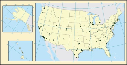
In forming the sample of liquidating national chains used in our identification, we include only those chains where upon bankruptcy all stores were closed and in which the retail chains operated in several states. Twenty-one cases in the data affect a total of 6,418 individual stores in our sample.13 The mean (median) number of stores of these retail chains is 305.6 (113) and ranges from 18 stores (KS Merchandise Mart) to 2,831 (Movie Gallery). All retail chains operate in more than one state, with the least diversified chain operating in only two states (Joe’s Sports Outdoors More) and the most geographically dispersed chain operating in all fifty states (Movie Gallery). Finally, as the last two columns of Table A1 demonstrate, all chains, except for Joe’s Sports Outdoors More, operate in more than one region of the United States. For example, eight chains have operations in all nine census divisions, and 19 of the 21 retail chain operate stores in at least four different census divisions. While two retailers seem to be less geographically dispersed (Joe’s Sports Outdoors More and Gottschalks), they do not drive our results and excluding them from the calculation of liquidated stores does not affect our findings. Furthermore, Figures 5, 6, and 7 illustrate the geographical dispersion of the initial stores locations of three firms that ended up in full liquidation used in the empirical identification: Circuit City, Linens ’N Things, and The Sharper Image. As the figures demonstrate, and consistent with the statistics in Table A1, these retail companies had dispersed geographical operation.
Stores locations for Circuit City
Stores locations for Linens ’N Things
Stores locations for The Sharper Image
Given their geographic dispersion, it is unlikely that the collapse of these chains is driven by localized economic shocks related to a particular store or subarea. Of course, this does not rule out the concern that nationwide, liquidating stores were positioned in worse locations. We address this concern in the next section.
3.2 Initial location of liquidated chain stores
The previous section presents evidence that most liquidated chains are geographically dispersed across states and U.S. regions. In this section we show that stores of liquidated chains were not located in ZIP codes with worse economic characteristics than the location of stores operated by nonbankrupt chains. We start by comparing the means of several local economic indicators between chains that fully liquidated and chains with similar business that avoid bankruptcy during the sample period. The local economic indicators that we use are the natural log of adjusted gross income at the ZIP code in 2006; the natural log of median house value at the ZIP code in the 2000 Census; and the percentage change in median house price during the period 2002–2006 in the ZIP code, which is based on data from Zillow. We focus on 2006, because an economic slowdown had already begun in 2007.
It is important to note that we compare the locations of chains to otherwise similar chains 2 years before the liquidated chains file for bankruptcy. We present summary statistics for the three chains presented in Figures 5, 6, and 7: Circuit City, Linens ’N Things, and The Sharper Image. Each of the chains is matched to a similar chain that avoided bankruptcy and liquidation during the sample period. We compare Circuit City to Best Buy; Linens ’N Things to Bed Bath & Beyond; and The Sharper Image to Brookstone. Table 3 illustrates no statistically significant differences in the three local economic indicators that pertain to store locations between the chains that will liquidate and their comparable chains.
Comparison of store locations
| Company | log(adjusted gross income) | log(median house value) | |$\Delta$|(house value 2002–2006) | Number of stores |
|---|---|---|---|---|
| Circuit City stores | 4.08 | 11.81 | 0.63 | 607 |
| Best Buy | 4.09 | 11.82 | 0.60 | 729 |
| p-value | (.799) | (.625) | (.164) | |
| Linens ’N Things | 4.12 | 11.91 | 0.61 | 511 |
| Bed Bath & Beyond | 4.11 | 11.87 | 0.60 | 700 |
| p-value | (.308) | (.119) | (.598) | |
| The Sharper Image | 4.17 | 12.19 | 0.68 | 181 |
| Brookstone | 4.16 | 12.02 | 0.69 | 269 |
| p-value | (.983) | (.00) | (.635) |
This table compares the means of log(adjusted gross income), log(median house value), and |$\Delta$|(house value 2002–2006) across all the stores of fully liquidated chains and similar chains that were not liquidated for three selected chains. Means are calculated based on store locations in 2006. p-values are calculated using a two-sample difference-in-means t-test.
Determinants of store locations
| (1) | (2) | (3) | (4) | (5) | (6) | |
|---|---|---|---|---|---|---|
| All stores | Nonmall stores | Mall stores | All stores | Nonmall stores | Mall stores | |
| log(median household income) | 0.0067 | 0.010 | –0.017 | –0.007 | 0.001 | –0.035 |
| (0.009) | (0.010) | (0.035) | (0.007) | (0.001) | (0.030) | |
| log(median house value) | 0.002 | 0.004 | –0.010 | 0.008*** | 0.010*** | –0.007 |
| (0.003) | (0.003) | (0.011) | (0.002) | (0.002) | (0.008) | |
| Median house price growth, | 0.0002 | –0.0004 | –0.003 | –0.001 | –0.001 | –0.003 |
| 2002–2006 | (0.004) | (0.004) | (0.016) | (0.003) | (0.003) | (0.009) |
| Mall | 0.037*** | 0.028*** | ||||
| (0.003) | (0.002) | |||||
| Year | 2005 | 2005 | 2005 | 2006 | 2006 | 2006 |
| Fixed effects | County | County | County | County | County | County |
| Observations | 52,597 | 44,488 | 8,109 | 76,057 | 62,808 | 13,249 |
| Adjusted |$R^{2}$| | .013 | .010 | .043 | .002 | .007 | .030 |
This table presents coefficient estimates and standard errors in parentheses for linear probability models of stores locations in 2005 (Columns 1–3) and 2006 (Columns 4–6). The table uses ZIP-code-level economic controls. Columns 1 and 4 use data on all stores; Columns 2 and 5 use data on stores that are not located in shopping malls; and Columns 3 and 6 only focus on stores located in malls. All regressions include an intercept and county fixed effects (data not reported). Standard errors are calculated by clustering at the ZIP code level. ***|$p<.01$|.
The first column of Table 4 demonstrates that stores of national retail chains liquidated after 2005 were located in ZIP codes with economic characteristics that are not statistically different from the ZIP codes of stores belonging to chains that avoided liquidation. The only difference between stores of chains that end in liquidations and other stores is that the former are more likely to be located in shopping malls. In Columns 2 and 3 of Table 4 we split the sample between nonmall stores (Column 2) and stores located in a mall (Column 3). Table 4 illustrates that store locations of chains that fully liquidated are again not different from the location of other stores when we stratify the data by a mall indicator.
Columns 4, 5, and 6 repeat the store location analysis in Columns 1, 2, and 3 but for 2006, rather than 2005. Again, the results show that stores of liquidated retail chains were located in ZIP codes similar to the location of other stores in terms of median household income and house price appreciation. The table demonstrates that the difference between the location of liquidated chain stores and the location of nonliquidated chain stores is that stores of liquidated chains are located in ZIP codes with slightly higher median house values in 2000.
In summary, Table 4 demonstrates that, along the observables, there are no significant differences between the location of liquidated chain stores and the location of stores belonging to retail chains that do not undergo liquidation in 2005. Moreover, the only slight difference in terms of location is that liquidated chain stores are more likely to be located in ZIP codes with slightly higher median house values in 2006. These results confirm that the initial location of stores of national chains that liquidated is not a likely cause of their failure. Thus, given the geographical dispersion of these chains and the ZIP codes in which they are located, these store closures are unlikely to be driven by worse local economic conditions. However, one remaining concern is that the locations of liquidating national chains suffered more during the economic downturn even though their initial location was no worse. As discussed below we address this point directly through the inclusion ZIP-code-by-year fixed effects.
4. Effect of Bankruptcy on Store Closures
4.1 Baseline regressions
We begin with a simple test of the negative externalities hypothesis by estimating a linear probability model of store closures conditional on the liquidation of neighboring stores that result from a national retailer chain-wide liquidation. We estimate different variants of the following baseline specification.
Neighboring bankrupt stores and store closures
| (1) | (2) | (3) | (4) | (5) | (6) | |
|---|---|---|---|---|---|---|
| Full liquidation bankrupt stores closures|$_{t-1}$| | ||||||
| |$\quad$| Same address | 0.0036** | 0.0037** | 0.0042*** | 0.0065*** | 0.0030** | 0.005*** |
| (0.002) | (0.002) | (0.002) | (0.002) | (0.0015) | (0.002) | |
| |$\quad$| Distance |$\le$| 50 m | 0.0003 | 0.0005 | 0.0002 | –0.0024 | –0.001 | –0.002 |
| (0.002) | (0.002) | (0.002) | (0.002) | (0.002) | (0.002) | |
| |$\quad$| 50 m |$<$| distance |$\le$| 100 m | 0.0019 | 0.0024 | 0.0022 | 0.0007 | 0.002 | 0.003 |
| (0.003) | (0.003) | (0.003) | (0.003) | (0.003) | (0.003) | |
| ln(income per household) | 0.0066*** | 0.0052*** | –0.0049 | –0.0650*** | 0.005*** | |
| (0.002) | (0.002) | (0.003) | (0.009) | (0.002) | ||
| Income growth | –0.0328*** | –0.0381*** | –0.0304*** | 0.0071 | –0.038*** | |
| (0.009) | (0.009) | (0.009) | (0.011) | (0.010) | ||
| Fixed effects | Year | Year+State | Year+County | Year+ZIP | Year-by-County | Year-by-ZIP |
| Observations | 654,581 | 654,581 | 654,581 | 654,581 | 654,581 | 654,581 |
| Adjusted |$R^{2}$| | .021 | .021 | .027 | .062 | .050 | .068 |
This table presents coefficient estimates and standard errors in parentheses for linear probability models of store closures. The dependent variable is an indicator variable equal to 1 if a store is closed in a given year, and 0 otherwise. The main explanatory variables—n(same address), n(0|$<$|distance|$\le$|50), and n(50|$<$|distance|$\le$|100)—are the number of stores that were closed in bankruptcies of chains that were fully liquidated and are (1) located at the same address; (2) located at a different address but within a 50-m radius of the store under consideration; and (3) located within a radius of more than 50 m but less than 100 m from the store under consideration, respectively. log(income per household) is a ZIP-code-level median adjusted gross income per capita; income growth is the annual growth rate in adjusted gross income per household within a ZIP code, both income measures are constructed from the IRS data. All regressions include an intercept and year fixed effects. Columns 2, 3, and 4 include state, county, and ZIP code fixed effects, respectively. Column 5 includes county*year, and Column 6 includes ZIP*year fixed effects. Standard errors are calculated by clustering at the ZIP code level. *|$p<.01$|; **|$p<.05$|; ***|$p<.001$|.
Column 1 of Table 5 presents the results of regression (2) using only year fixed effects. As can be seen, there is a positive relation between the number of stores closed as part of a national chain-wide liquidation and the probability that stores of nonbankrupt firms in the same address will close.14 Thus, consistent with the externalities conjecture, increases in bankruptcies and store closures are associated with further closings of neighboring stores. The effect is economically sizable: being located at the same address as a liquidating retail-chain store increases the probability of closure by 0.36 percentage points, or 5.9% of the sample mean. We also find that the negative effect of store closures is confined to stores located at the same address given that the coefficients on both n(0|$<$|distance|$\le$|50) and n(50|$<$|distance|$\le$|100) are not statistically different from zero. As shown below, once heterogeneity is added to the analysis we capture effects at longer distances.
Column 2 of the table repeats the analysis in Column 1, while adding state fixed effects to the specification. As can be seen, the results remain qualitatively and quantitatively unchanged: bankruptcy induced stores closures lead to additional closings of stores in the same area. Columns 3 and 4 repeat the analysis but add either county or ZIP code fixed effects to the specification and hence control for unobserved heterogeneity at a finer geographical level. As can be seen in the table, we continue to find a positive relation between stores that are closed in full liquidation bankruptcies and subsequent store closures in the same address.
Further, the inclusion of either county or ZIP code fixed effects increases the marginal effect of same address store closures considerably from 0.0036 and 0.0037 to 0.0042 and 0.0065 in the county and ZIP fixed effects specifications, respectively. Thus, Table 5 demonstrates that having one neighboring store close down as part of a national retail liquidation increases the likelihood that stores in the same address will close by between 5.9% and 10.7% relative to the unconditional mean.15 The results point to agglomeration economies in retail, as the reduction of store density in a given locality exhibits a negative effect on other stores in the area, increasing their likelihood of closure. This is consistent with evidence in Gould and Pashigian (1998) and Gould, Pashigian, and Prendergast (2005), who show that store-level sales may depend on the sales of neighboring stores.16
Finally, Columns 5 and 6 include county-by-year or ZIP-code-by-year fixed effects and hence control for unobserved time-varying heterogeneity at a finer geographical level. The inclusion of these fixed effects soaks up any time-varying local economic conditions that may be correlated with the likelihood of store closures. As can be seen in Columns 5 and 6, we continue to find a positive relation between stores that are closed in full liquidation bankruptcies and subsequent store closures in the same address. These results alleviate concerns that the locations of liquidating national chains suffered more during the economic downturn even though their initial location was no worse.
Turning to the control variables in Table 5, in the first three columns the coefficient of log(income per household) is either positive or not statistically significant in explaining individual store closures. Moreover, as would be expected, the first three columns of Table 5 also suggest that stores are less likely to be closed in ZIP codes in which income grows over time. Furthermore, in our specifications that include ZIP code fixed effects in which we control for unobserved geographical heterogeneity at a finer level (Column 4) we find that income per household has a negative and significant effect on the likelihood that a store closes down, again, as one would expect.
4.1.1 Neighboring bankrupt stores and closing of stores by distance
Table 6 reports the results of regression (3) using the fixed effects specifications employed in Table 5. As the table demonstrates, out of the eleven distance measures, |$\beta_{1}$|—the coefficient on n(same address)—is the only estimate that is consistently statistically and economically significant. While |$\beta_{1}$| ranges from 0.004 (in the year fixed effects specification) to 0.007 (in the ZIP code fixed effects specification), almost all of the other estimates are far smaller and are not statistically different from zero. Only the coefficient on n(300|$<$|distance|$\le$|350) is negative and marginally significant in one specification out of five while the coefficient on n(400|$<$|distance|$\le$|450) is positive and marginally significant in the ZIP-code-by-year fixed effects regression. The results in Table 6 confirm our baseline results and demonstrate that when analyzing average effects the negative externality of store closures is mostly driven by very near stores even when we control for unobserved time-varying heterogeneity. However, we return to this result below when analyzing the externality effect of store closures on neighboring stores belonging to chains of differing financial health and differing industries.
Neighboring bankrupt stores and store closures by distance
| (1) | (2) | (3) | (4) | (5) | ||||
|---|---|---|---|---|---|---|---|---|
| Full liquidation bankrupt stores closures|$_{t-1}$| | ||||||||
| |$\quad$| Same address | 0.004** | 0.004** | 0.004*** | 0.007*** | 0.006*** | |||
| (0.002) | (0.002) | (0.002) | (0.002) | (0.02) | ||||
| |$\quad$| Distance |$\le$| 50 m | 0.0002 | 0.0004 | 0.0002 | –0.002 | –0.003 | |||
| (0.002) | (0.002) | (0.002) | (0.002) | (0.003) | ||||
| |$\quad$| 50 m |$<$| distance |$\le$| 100 m | 0.002 | 0.002 | 0.002 | 0.001 | 0.003 | |||
| (0.003) | (0.003) | (0.003) | (0.003) | (0.003) | ||||
| |$\quad$| 100 m |$<$| distance |$\le$| 150 m | 0.002 | 0.002 | 0.002 | 0.002 | 0.002 | |||
| (0.004) | (0.004) | (0.004) | (0.005) | (0.005) | ||||
| |$\quad$| 150 m |$<$| distance |$\le$| 200 m | 0.003 | 0.003 | 0.002 | 0.001 | 0.003 | |||
| (0.005) | (0.005) | (0.005) | (0.005) | (0.005) | ||||
| |$\quad$| 200 m |$<$| distance |$\le$| 250 m | –0.001 | –0.000 | –0.000 | –0.003 | –0.003 | |||
| (0.003) | (0.003) | (0.003) | (0.003) | (0.004) | ||||
| |$\quad$| 250 m |$<$| distance |$\le$| 300 m | 0.003 | 0.004 | 0.003 | 0.001 | 0.001 | |||
| (0.004) | (0.004) | (0.004) | (0.004) | (0.004) | ||||
| |$\quad$| 300 m |$<$| distance |$\le$| 350 m | –0.003 | –0.002 | –0.003 | –0.005* | –0.003 | |||
| (0.003) | (0.003) | (0.003) | (0.003) | (0.004) | ||||
| |$\quad$| 350 m |$<$| distance |$\le$| 400 m | 0.002 | 0.003 | 0.003 | 0.000 | 0.004 | |||
| (0.003) | (0.003) | (0.003) | (0.003) | (0.003) | ||||
| |$\quad$| 400 m |$<$| distance |$\le$| 450 m | 0.004 | 0.005 | 0.004 | 0.001 | 0.006* | |||
| (0.004) | (0.004) | (0.003) | (0.003) | (0.004) | ||||
| |$\quad$| 450 m |$<$| distance |$\le$| 500 m | 0.005 | 0.005 | 0.002 | –0.001 | –0.0001 | |||
| (0.007) | (0.007) | (0.006) | (0.006) | (0.006) | ||||
| ln(income per household) | 0.007*** | 0.005*** | –0.005 | –0.065*** | ||||
| (0.002) | (0.002) | (0.003) | (0.009) | |||||
| Income growth | –0.033*** | –0.038*** | –0.030*** | 0.007 | ||||
| (0.009) | (0.009) | (0.009) | (0.011) | |||||
| Fixed effects | Year | Year+State | Year+County | Year+ZIP | Year-by-ZIP | |||
| Observations | 654,581 | 654,581 | 654,581 | 654,581 | 654,581 | |||
| Adjusted |$R^{2}$| | .021 | .022 | .027 | .062 | .065 | |||
This table presents coefficient estimates and standard errors in parentheses for linear probability models of store closures. The dependent variable is an indicator variable equal to 1 if a store is closed in a given year, and 0 otherwise. The explanatory variables are the number of stores that were closed in bankruptcies of chains that were fully liquidated in different distance ranges ranging from same address up to 500 m in increments of 50 m. log(income per household) is a ZIP-code-level median-adjusted gross income per capita; income growth is the annual growth rate in adjusted gross income per household within a ZIP code, both income measures are constructed from the IRS data. All regressions include an intercept and year fixed effects. Columns 2, 3, and 4 include state, county, and ZIP code fixed effects, respectively. Column 5 includes ZIP*year fixed effects. Standard errors are calculated by clustering at the ZIP code level. *|$p<.01$|; **|$p<.05$|; ***|$p<.001$|.
We also estimate the externalities effects using a continuous distance measure between the affected stores and a neighboring store that is liquidated in as part of a national retail chain full liquidation bankruptcy. We use two measures: (1) the distance (in kilometers) to the nearest liquidated store; and (2) the average distance to the three nearest liquidated stores. Given that the externality effects are present only for neighboring stores, we estimate these regressions conditioning on the distance to the nearest liquidated store being less than 1 km. We report the results in Table A2.
There are 71,089 store-year observations that are exposed to at least one store closure in a national chain bankruptcy liquidation within 1 km of their location (Columns 1 and 2) and 11,586 store-year observations that are exposed to three such liquidating stores with the average distance to these three stores not exceeding 1 km (Columns 3 and 4). Table A1 demonstrates that the likelihood of a store closure declines with the distance to the liquidated store. For example, using the estimates in Column 2, which include ZIP-code-by-year fixed effects, a liquidated store that is 500 m away reduces the likelihood of a store closure relative to a store that is 50 m away by 0.006*0.5-0.006*0.05 |$=$| 0.0027, implying a reduction in the probability of a closure of 7.4% relative to the conditional mean.17 The effect is stronger for stores that are in the vicinity of three liquidated stores. The estimates in Column 4 imply that a liquidated store that is 500 away reduces the likelihood of a store closure relative to a store that is 50 m away by 0.015*0.5-0.015*0.05 = 0.007, corresponding to a reduction in the probability of closure of 20.1%.
4.2 Falsification exercise: Placebo regressions
We supplement our analysis by performing a placebo exercise, the results of which are reported in Table 7. For each of the distance measures in Regression (2) and Table 5 we define a “placebo” variable, which, for each store in our sample, counts the number of neighboring stores that are part of a national chain that will liquidate in the future but are currently not in liquidation. In particular, we count the number of neighboring stores that are part of a national chain that will liquidate in 2 years but that are currently not in liquidation.18
Neighboring bankrupt stores and placebo store closures
| (1) | (2) | (3) | (4) | |
|---|---|---|---|---|
| Full liquidation bankrupt stores closures|$_{t-1}$| | ||||
| |$\quad$| Same address | 0.003* | 0.0032** | 0.005*** | 0.006*** |
| (0.002) | (0.0016) | (0.0017) | (0.0021) | |
| |$\quad$| Distance |$\le$| 50 m | 0.001 | 0.0002 | –0.002 | –0.001 |
| (0.002) | (0.002) | (0.003) | (0.0025) | |
| |$\quad$| 50 m |$<$| distance |$\le$| 100 m | 0.002 | 0.001 | –0.001 | 0.002 |
| (0.003) | (0.003) | (0.003) | (0.003) | |
| Placebo full liquidation bankrupt stores closures|$_{t+2}$| | ||||
| |$\quad$| Same address | –0.008*** | –0.007*** | –0.0035 | –0.0027 |
| (0.002) | (0.002) | (0.002) | (0.0029) | |
| |$\quad$| Distance |$\le$| 50 m | –0.0022 | –0.002 | 0.001 | 0.001 |
| (0.003) | (0.003) | (0.003) | (0.003) | |
| |$\quad$| 50 m |$<$| distance |$\le$| 100 m | –0.008*** | –0.008** | –0.0056* | –0.005 |
| (0.003) | (0.003) | (0.003) | (0.0033) | |
| ln(income per household) | 0.0058*** | –0.0043 | –0.066*** | |
| (0.002) | (0.003) | (0.009) | ||
| Income growth | –0.0318*** | –0.030*** | 0.009 | |
| (0.008) | (0.009) | (0.011) | ||
| Fixed effects | Year+State | Year+County | Year+ZIP | Year-by-ZIP |
| Observations | 654,581 | 654,581 | 654,581 | 654,581 |
| Adjusted |$R^{2}$| | .022 | .025 | .040 | .069 |
This table presents coefficient estimates and standard errors in parentheses for linear probability models of store closures. The dependent variable is an indicator variable equal to 1 if a store is closed in a given year, and 0 otherwise. The main explanatory variables—n(same address), n(0|$<$|distance|$\le$|50) and n(50|$<$|distance|$\le$|100)—are the number of stores that were closed in bankruptcies of chains that were fully liquidated and are (1) located at the same address; (2) located at a different address but are within a 50-m radius of the store under consideration; and (3) located within a radius of more than 50 m but less than 100 m from the store under consideration, respectively. The first three variables are the lagged store closure countervariables, and the following three variables are the forwarded store closure countervariables. log(income per household) is a ZIP-code-level median-adjusted gross income per capita; income growth is the annual growth rate in adjusted gross income per household within a ZIP code, both income measures are constructed from the IRS data. All regressions include an intercept and year fixed effects. Columns 1, 2, and 3 include state, county, and ZIP code fixed effects, respectively. Column 4 includes county*year, and Column 6 includes ZIP*year fixed effects. Standard errors are calculated by clustering at the ZIP code level. *|$p<.01$|; **|$p<.05$|; ***|$p<.001$|.
As can be seen in Table 7, the results are consistent with an externality effect. The coefficients on the lagged variables, |$\beta_{1}, \beta_{2}$|, and |$\beta_{3}$|, are identical to our baseline results in Table 5. The coefficient on the fourth and sixth variables—that is, the forwarded n(same address)|$_{i,t+2}$| , and forwarded n(50|$<$|distance|$\le$|100)|$_{i,t+1}$|—are negative and significant in the first two models. However, once we move to the preferred specification, which includes ZIP-code-by-year fixed effects, these coefficients become smaller and are no longer statistically significant. Taken together, the results show that the effect of store liquidation on subsequent store closures is not driven by the location of the retail-chain stores that will later become bankrupt but rather by the timing in which they were actually closed.
4.3 Neighboring bankrupt stores and local economic conditions
That the results presented in Table 5 are robust to the inclusion of ZIP-code-by-year fixed effects enables us to control for unobserved time-varying heterogeneity at the ZIP code level. The ZIP-code-by-year fixed effects specification is useful in addressing omitted variables, but it does not flesh out the potential heterogeneous effects of local economic conditions on store closures. Is it the case, for example, that the negative externality imposed by store liquidations is different in magnitude across poorer versus more affluent areas? To what extent does this negative externality depend on local economic conditions?
In Table 8 we investigate the effect of local economic conditions on store closures using two important indicators of the local economy: (1) the median house price level in 2000 and (2) the change in house prices from 2002 to 2006, both measured at the ZIP code level. We conduct a split-sample analysis based on these variables and reestimate regression (2) separately in each subsample. As Table 8 shows, the effect of n(same address) is positive and statistically significant in both ZIP codes below the median house price change from 2002 to 2006 (Column 1) and in ZIP codes above the median (Column 2). Likewise, the effect of n(same address) is positive and statistically significant in ZIP codes above and below the median house price level in 2000, although the effect is smaller in ZIP codes with higher house prices. That is, the negative externality imposed by store liquidations exists also in more affluent ZIP codes.
Neighboring bankrupt stores: Sample splits by local economic conditions
| (1) | (2) | (3) | (4) | |
|---|---|---|---|---|
| House price change|$_{2002-2006}$| | House price|$_{2000}$| | |||
| Below median | Above median | Below median | Above median | |
| |$\quad$| Same address | 0.006* | 0.007*** | 0.008*** | 0.004** |
| (0.031) | (0.003) | (0.026) | (0.002) | |
| |$\quad$| Distance |$\le$| 50 m | –0.004 | 0.006 | 0.002 | –0.002 |
| (0.004) | (0.004) | (0.003) | (0.003) | |
| |$\quad$| 50 m |$<$| distance | 0.001 | –0.00003 | 0.007 | –0.001 |
| |$\le$| 100 m | (0.005) | (0.004) | (0.004) | (0.003) |
| Fixed effects | Year- | Year- | Year- | Year- |
| by-ZIP | by-ZIP | by-ZIP | by-ZIP | |
| Observations | 206,897 | 205,170 | 324,345 | 325,649 |
| Adjusted |$R^{2}$| | .048 | .046 | .049 | .053 |
This table presents coefficient estimates and standard errors in parentheses for linear probability models of store closures. The dependent variable is an indicator variable equal to 1 if a store is closed in a given year, and 0 otherwise. The main explanatory variables–n(same address), n(0|$<$|distance|$\le$|50), and n(50|$<$|distance|$\le$|100)—are the number of stores that were closed in bankruptcies of chains that were fully liquidated and are (1) located at the same address; (2) located at a different address but are within a 50-m radius of the store under consideration; and (3) located within a radius of more than 50 m but less than 100 m from the store under consideration, respectively. Regressions are estimated separately for ZIP codes below (Column 1) and above (Column 2) the median house price change from 2002 to 2006 and below (Column 3) and above (Column 4) the median house price in 2000. All regressions include an intercept and ZIP*year fixed effects. Standard errors are calculated by clustering at the ZIP code level. *|$p<.01$|; **|$p<.05$|; ***|$p<.001$|.
To further test the effects of neighboring store closures conditional on local economic conditions we interact each of our three measures n(same address), n(0|$<$|distance|$\le$|50), and n(50|$<$|distance|$\le$|100) with |$log(income\,per\,household)_{i,t}$| measured at the ZIP code level and report results in Table 9. As the table illustrates, conditional on store closures, the likelihood that neighboring stores close as well declines when local economic conditions are better. That is, the negative externality of store closures diminishes with the strength of local economic conditions. For example, at the 25th percentile of |$log(income\,per\,household)$| and using the estimates from Column 3 with ZIP-code-by-year fixed effects, being located at the same address as a liquidating retail-chain store increases the probability of store closure by 0.870 percentage points, or 14.3% of the sample mean. In contrast, the same effect at the 75th percentile of |$log(income\,per\,household)$| increases store closure probability by 0.438 percentage points, or 7.2% of the sample mean.19
Neighboring bankrupt stores: The effect of economic conditions on store closures
| (1) | (2) | (3) | (4) | (5) | |
|---|---|---|---|---|---|
| Sample period | 2006–2009 | 2006–2009 | 2006–2009 | 2006–2007 | 2008–2009 |
| |$\quad$| Same address | 0.083*** | 0.086*** | 0.066** | 0.067 | 0.068* |
| (0.023) | (0.022) | (0.030) | (0.054) | (0.037) | |
| |$\quad$||$\times$|ln(income per household) | –0.0199*** | –0.021*** | –0.015** | –0.016 | –0.015* |
| (0.006) | (0.005) | (0.008) | (0.013) | (0.009) | |
| |$\quad$| Distance |$\le$| 50 m | 0.014 | 0.009 | 0.050 | 0.151** | 0.023 |
| (0.040) | (0.040) | (0.049) | (0.073) | (0.056) | |
| |$\quad$||$\times$|ln(income per household) | –0.003 | –0.002 | –0.013 | –0.037** | –0.006 |
| (0.010) | (0.010) | (0.012) | (0.018) | (0.014) | |
| |$\quad$| 50 m |$<$| distance | –0.009 | –0.014 | –0.007 | –0.147 | 0.023 |
| |$\le$| 100 m | (0.046) | (0.005) | (0.049) | (0.100) | (0.057) |
| |$\quad$||$\times$|ln(income per household) | –0.004 | 0.004 | 0.0022 | 0.037 | –0.005 |
| (0.003) | (0.012) | (0.013) | (0.025) | (0.014) | |
| ln(income per household) | –0.004 | 0.006*** | |||
| (0.003) | (0.002) | ||||
| Income growth | –0.030*** | –0.039*** | |||
| (0.009) | (0.010) | ||||
| Fixed effects | Year+ | Year- | Year- | Year- | Year- |
| County | by-County | by-ZIP | by-ZIP | by-ZIP | |
| Observations | 654,581 | 654,581 | 654,581 | 271,260 | 378,460 |
| Adjusted |$R^{2}$| | .025 | .026 | .058 | .06 | .05 |
This table presents coefficient estimates and standard errors in parentheses for linear probability models of store closures. The dependent variable is an indicator variable equal to 1 if a store is closed in a given year, and 0 otherwise. The main explanatory variables—n(same address), n(0|$<$|distance|$\le$|50), and n(50|$<$|distance|$\le$|100)—are the number of stores that were closed in bankruptcies of chains that were fully liquidated and are (1) located at the same address; (2) located at a different address but are within a 50-m radius of the store under consideration; and (3) located within a radius of more than 50 m but less than 100 m from the store under consideration, respectively. Each of the three store closure number variables are also interacted with log(income per capita). log(income per household) is a ZIP-code-level median-adjusted gross income per capita; income growth is the annual growth rate in adjusted gross income per household within a ZIP code, both income measures are constructed from the IRS data. The regressions are estimated separately for 2006–2009 (Columns 1–3), 2006–2007 (Column 4), and 2008–2009 (Column 5) subperiods. All regressions include an intercept. Column 1 includes year and county fixed effects; Column 2 includes county*year fixed effects; and Columns 3, 4, and 5 include ZIP*year fixed effects. Standard errors are calculated by clustering at the ZIP code level. *|$p<.01$|; **|$p<.05$|; ***|$p<.001$|.
Importantly, while the effect of neighboring store closures is smaller in areas with better economic conditions, the effect is still positive and significant over the vast majority of the household income distribution. Indeed, the estimates show that so long as the ZIP code level |$log(income\,per\,household)$| is lower than the 93rd percentile of ZIP code income distribution (corresponding to ZIP codes with an adjusted gross income per household of
One potential explanation for the fact that the negative externality of store closures is more pronounced in lower income areas is that store owners in these areas find it more difficult to raise external capital to smooth the negative shock imposed by the diseconomies of agglomeration caused by the liquidation of the retail chain store. Facing costly external finance (or a lack of financing), the owner thus closes the store. Alternatively, it could be that stores in lower-income areas have lower economic value, so that the shock imposed by the negative externality is more likely to push these stores toward nonviability. Regardless, as stated above, the results show a negative externality, albeit of weaker magnitude, even in more affluent areas.
4.4 Store closures and the business cycle
Our sample period from 2005 to 2010 encompasses the Great Recession. In this subsection, we exploit our empirical strategy to analyze the effect of the liquidation of retail chains on neighboring store closures across the business cycle.20 To this end, we split our sample into the precrisis period (2006–2007) and the recession period (2008–2009), estimating the effects of neighboring store closures in each period separately.21
Most of the bankruptcies listed in Table A1 cluster during the 2008–2009 recession period in which many retailers failed and were liquidated. Nevertheless, a number of bankruptcy and full liquidation cases are present in the 2006–2007 precrisis period, and we use them in our analysis below. Importantly, that many bankruptcies are clustered during the crisis period does not imply that our results on the negative externality of store liquidations are driven by this single, large economic shock. The identification strategy exploits local level variation, which depend on the proximity of stores to the stores of liquidating retail chains. Indeed, the fact that we do not find results at larger distances speaks against a common shock driving all store closures.22
In the last two columns of Table 9 we interact each of our three measures of proximity to liquidated firms—n(same address), n(0|$<$|distance|$\le$|50) and n(50|$<$|distance|$\le$|100)—with log(income per household), but do so separately for the precrisis (Column 4) and crisis (Column 5) period using year-by-ZIP-code fixed effects.
The smaller number of firm-wide liquidations during the precrisis period naturally leads to a reduction in statistical power in estimating our regression specifications during the precrisis years. When we include ZIP and year fixed effects (not reported for brevity) the association between store closures and an increased likelihood of neighboring store closures continues to hold during the precrisis period as well, with the negative externality declining as local economic conditions improve. Examining the relevant coefficients on n(same address), both the direct effect of store closures and the interacted effect with local economic conditions are similar in magnitudes in the two subperiods (crisis and noncrisis).23
Our empirical findings are, therefore, not driven solely by the 2008–2009 crisis period, with results holding during the 2006 and 2007 period before the onset of the Great Recession, in spite of the lower statistical power in the precrisis years. Of course, since liquidations themselves are more prevalent during recessions, the aggregate impact of the negative externality during these periods is likely to be larger. The destruction of local economies of agglomeration thus further amplifies negative shocks occurring during downturns.
4.5 Stores closings inside shopping malls
Prior work has shown that anchor stores in shopping malls create positive externalities on other nonanchor stores by attracting customer traffic. Mall owners internalize this externality by providing rent subsidies to anchor stores. Indeed, the rent subsidy provided to anchor stores as compared to nonanchor stores—estimated at no less than 72%—suggests that these positive externalities are economically large. Given the importance of anchor stores within malls, we next focus our analysis on the potential externalities that arise when an anchor store in a shopping mall closes. To maintain our identification strategy, we focus only on the effects of anchor store closures that are a result of the liquidation of a national retail chain.
We match our data on retail chain stores to Esri’s Major Shopping Centers, a panel data set of major U.S. shopping centers that lists the name and address of each of the malls and includes data on gross leasable area in the mall, the number of stores, and the names of up to four anchor tenants in the mall. There are 4,421 unique malls that are matched to 104,217 store-year observations. The average mall has a gross leasable area (GLA) of 474,019 square feet (median = 349,437) and ranges from a 25th percentile of 259,086 sq ft to a 75th percentile of 567,000 sq ft. The matched malls span all fifty states and the District of Columbia. Figure 8 presents the geographical distribution of the malls that are matched to our data and the shopping mall gross leasable area.
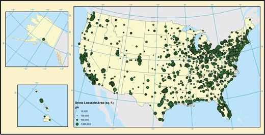
Locations and size of shopping malls
Next, to estimate the externality generated by store closures within malls, we rerun our baseline regressions only on stores that have been matched to the Esri Mall database. Similar to the baseline regressions, our main independent variable in this regression, same mall, is simply the number of retail-chain stores in the mall that close because of the liquidation of the entire chain. That our data enable us to control for mall fixed effects (as opposed to just ZIP code fixed effects) in addition to the year dummies further alleviates concerns about the initial location of stores of chains that liquidated.24
As Column 1 of Table 10 shows, we find that store closings in a mall lead to further store closures within a mall. When a store closes in a mall, the subsequent annual closure rate of other stores in the mall increases by 0.3 percentage points, or 4.9% of the sample mean. In Column 2 we add a second variable that counts the number of anchor stores within a mall that are closed as a result of the liquidation of a national retail chain. As the table shows, we find that most of the effect within malls is coming from anchor stores: The coefficient on same mall becomes insignificant while that on the number of national liquidating anchor stores rises to 0.009. The effect of anchor store closure is thus triple that of the average effect of nonanchor stores, consistent with prior research pointing to the impact of anchor stores in drawing in customers. The economic effect is sizable with an anchor store closure causing a 14.7% increase in the probability of store closures within the mall relative to the unconditional mean.
Mall versus nonmall store closures
| (1) | (2) | (3) | (4) | (5) | |
|---|---|---|---|---|---|
| Mall stores | Nonmall stores | ||||
| |$\quad$| Same mall | 0.003* | 0.002 | |||
| (0.002) | (0.002) | ||||
| |$\quad$| Same mall anchor store | 0.009** | ||||
| (0.004) | |||||
| |$\quad$| Same address | 0.0115*** | 0.0087** | 0.0089** | ||
| (0.004) | (0.004) | (0.004) | |||
| |$\quad$| Distance |$\le$| 50 m | –0.0008 | –0.0034 | –0.001 | ||
| (0.003) | (0.003) | (0.003) | |||
| |$\quad$| 50 m |$<$| distance |$\le$| 100 m | 0.0060* | 0.0039 | 0.004 | ||
| (0.004) | (0.003) | (0.003) | |||
| ln(income per household) | –0.046* | –0.048* | –0.0023 | –0.0682*** | |
| (0.027) | (0.027) | (0.003) | (0.009) | ||
| Income growth | 0.094** | 0.095** | –0.0413*** | 0.0002 | |
| (0.038) | (0.038) | (0.010) | (0.011) | ||
| Fixed effects | Year+Mall | Year+Mall | Year+County | Year+ZIP | Year-by-ZIP |
| Observations | 104,217 | 104,217 | 550,364 | 550,364 | 550,364 |
| Adjusted |$R^{2}$| | .094 | .094 | .028 | .067 | .071 |
This table presents coefficient estimates and standard errors in parentheses for linear probability models of store closures. The dependent variable is an indicator variable equal to 1 if a store is closed in a given year, and 0 otherwise. In Columns 1 and 2, we focus on stores located in shopping malls, and the main dependent variables are same mall (the number of retail-chain stores in the mall that close because of the liquidation of the entire chain) and same mall anchor store (the number of anchor stores within a mall that are closed as a result of the liquidation of a national retail chain). In Columns 3 and 4, we focus on stores not located in shopping malls, and the main explanatory variables n(same address), n(0|$<$|distance|$\le$|50), and n(50|$<$|distance|$\le$|100) are the number of stores that were closed in bankruptcies of chains that were fully liquidated and are (1) located at the same address; (2) located at a different address but are within a 50-m radius of the store under consideration; and (3) located within a radius of more than 50 m but less than 100 m from the store under consideration, respectively. All regressions include an intercept. Columns 1 and 2 include year and mall fixed effects; Column 3 includes year and county fixed effects; Column 4 includes year and ZIP code fixed effects; and Column 5 includes ZIP*year fixed effects. Standard errors are calculated by clustering at the ZIP code level. *|$p<.01$|; **|$p<.05$|; ***|$p<.001$|.
One caveat that should be noted for this effect is that some firms add cotenancy clauses into their lease contracts, which provide them the option to terminate their leases when certain stores close. Thus, the increase in the externality effect could be explained by both the greater importance of anchor stores in drawing traffic to malls and the higher flexibility that fellow stores enjoy in terminating their leases when an anchor store closes.
In a separate set of regressions, we also analyze the effect of store closures on stores located outside malls. Columns 3–5 repeat our baseline analysis in Table 5 for stores that were not matched to the Esri’s Mall database. There are 550,364 stores in our data that are not part of matched malls. Such stores either are not located in shopping malls or are located in smaller malls not matched to the Esri Mall database. The table demonstrates that the coefficient on n(same address)|$_{i,t-1}$| is positive and significant statistically, indicating, once again, a negative externality of store closure on stores located at the same address.25 Comparing the coefficients on the same-address variable to within-mall estimates in Columns 1 and 2 indicates that the effect of store closure outside shopping malls on other stores located at the same address is similar to that of the effect of an anchor store closure.26 One potential reason for this is that because of the small number of stores in small shopping malls or in buildings where stores collocate, any store closure will have a relatively large impact on other stores nearby.27
5. Heterogeneity in the Response to Store Closures
To better understand the mechanisms through which store closures spread to further closing of stores, we add heterogeneity to our empirical analysis. In this section, we investigate the transmission of negative externalities that are imposed by bankruptcies of neighboring stores further by studying the differential effect of store closures along the following three peer characteristics: (1) across industries; (2) conditional on a firm’s financial strength; and (3) store size.
5.1 Effect of bankrupt stores by industry
We begin by analyzing whether the effect of store closures on neighboring store closures depends on the industrial composition of stores in the same vicinity. A number of spatial models of imperfect competition predict that firms will choose to locate as far as possible from their newest competitors (Chamberlin 1933; Nelson 1970; Salop 1979; Stuart 1979). The key result of these models is that when other stores are farther from a particular store, a specific store will have greater market power over the consumers located near it. If so-called “centrifugal competition” is the main factor driving stores locations in the United States, we should expect that store closures will benefit nearby stores that are in the same retail segment. This is simply because the remaining stores will face less competition.
Alternative spatial models suggest that it may be optimal for stores in the same industry to locate next to one another. According to this view, the geographical concentration of similar stores is driven by consumers’ imperfect information. For example, Wolinsky (1983, p. 274) writes “[I]mperfectly informed consumers are attracted to a cluster of stores because that is the best setting for search. A store may thus get more business and higher profits when it is located next to similar stores. This effect may outweigh centrifugal competitive forces |$\ldots$|.”
Indeed, research in urban economics have provided a good deal of evidence for the existence of economies of agglomeration and industrial clusters.28
To test how product substitutability and similarity influences the effect of retail store closures on neighboring retail stores, we use the North American Industry Classification System (NAICS) definition of an industry. To assign firms into industries, we employ two definitions that are based on five-digit and six-digit NAICS codes.29 Specifically, for each store in our sample, we define the same industry analogs of n(same address), n(0|$<$|distance|$\le$|50), and n(50|$<$|distance|$\le$|100), which count only the number of liquidating retail-chain stores in the same industry of the given store, where industry identity is defined using either five- or six-digit NAICS codes. For each store, we also define different industry exposures to stores of liquidating national retail chains in an analogous manner. We then estimate, separately, the effect of same industry and different industry store closures on subsequent store closings in their area. Table 11 presents results based on five-digit NAICS codes.
Bankrupt stores industry and store closures (five-digit NAICS)
| (1) | (2) | (3) | (4) | (5) | (6) | (7) | (8) | ||
|---|---|---|---|---|---|---|---|---|---|
| Full liquidation bankrupt stores closures same industry|$_{t-1}$| | |||||||||
| |$\quad$| Same address | 0.008* | 0.008* | 0.009** | 0.010** | |||||
| (0.004) | (0.004) | (0.004) | (0.004) | ||||||
| |$\quad$| Distance |$\le$| 50 | 0.022** | 0.022** | 0.018** | 0.024** | |||||
| (0.009) | (0.009) | (0.009) | (0.010) | ||||||
| |$\quad$| 50 |$<$| d |$\le$| 100 | 0.002 | 0.002 | –0.004 | 0.0025 | |||||
| (0.009) | (0.009) | (0.010) | (0.010) | ||||||
| Full liquidation bankrupt stores closures different industry|$_{t-1}$| | |||||||||
| |$\quad$| Same address | 0.003** | 0.004** | 0.006*** | 0.005** | |||||
| (0.002) | (0.002) | (0.002) | (0.002) | ||||||
| |$\quad$| Distance |$\le$| 50 | –0.001 | –0.001 | –0.004 | –0.003 | |||||
| (0.002) | (0.002) | (0.003) | (0.003) | ||||||
| |$\quad$| 50 |$<$| d |$\le$| 100 | 0.003 | 0.002 | 0.001 | 0.002 | |||||
| (0.003) | (0.003) | (0.003) | (0.003) | ||||||
| ln(income | 0.005*** | –0.005 | –0.066*** | 0.005*** | –0.005 | –0.065*** | |||
| per household) | (0.002) | (0.003) | (0.009) | (0.002) | (0.003) | (0.009) | |||
| Income growth | –0.038*** | –0.030*** | 0.007 | –0.038*** | –0.030*** | 0.007 | |||
| (0.009) | (0.009) | (0.011) | (0.009) | (0.009) | (0.011) | ||||
| Fixed effects | Year+ | Year+ | Year+ | Year-by-ZIP | Year+ | Year+ | Year+ | Year-by-ZIP | |
| State | County | ZIP | State | County | ZIP | ||||
| Observations | 654,581 | 654,581 | 654,581 | 654,581 | 654,581 | 654,581 | 654,581 | 654,581 | |
| Adjusted |$R^2$| | .022 | .027 | .062 | .071 | .022 | .027 | .062 | .070 | |
This table presents coefficient estimates and standard errors in parentheses for linear probability models of store closures. The dependent variable is an indicator variable equal to 1 if a store is closed in a given year, and 0 otherwise. The main explanatory variables—n(same address), n(0|$<$|distance|$\le$|50), and n(50|$<$|distance|$\le$|100)—are the number of stores that were closed in bankruptcies of chains that were fully liquidated and are (1) located at the same address; (2) located at a different address but are within a 50-m radius of the store under consideration; and (3) located within a radius of more than 50 m but less than 100 m from the store under consideration, respectively. Columns 1–4 report results from estimating regressions in which for each store in our sample we define same industry analogs of n(same address), n(0|$<$|distance|$\le$|50), and n(50|$<$|distance|$\le$|100), which count only the number of liquidating retail-chain stores that are in the same industry of the given store, where industry identity is defined at the five-digit NAICS. Columns 5 and 6 report results from estimating regressions in which analogs of n(same address), n(0|$<$|distance|$\le$|50), and n(50|$<$|distance|$\le$|100) are defined as different industry exposures to stores of liquidating national retail chains. log(income per household) is a ZIP-code-level median-adjusted gross income per capita; income growth is the annual growth rate in adjusted gross income per household within a ZIP code, both income measures are constructed from the IRS data. All regressions include an intercept and year fixed effects. Columns 1, 2, and 3 include state, county, and ZIP code fixed effects, respectively. Column 4 includes ZIP*year fixed effects. Likewise, Columns 5, 6, and 7 include state, county, and ZIP code fixed effects, respectively, and Column 8 includes ZIP*year fixed effects. Standard errors are calculated by clustering at the ZIP code level. *|$p<.01$|; **|$p<.05$|; ***|$p<.001$|.
As the table shows, we find that the effect of same industry store closures is larger than different industry store closures. For example, in the specification that controls for ZIP-code-by-year fixed effects we find that the coefficient on n(same address) is 0.01 for same industry compared to 0.005 in the different industry regression. Moreover, we also find a positive and significant effect of our second distance measure, n(0|$<$|distance|$\le$|50), in the same industry regressions. This effect is quite sizable: the coefficient of 0.024 (significant at the 5% level) in Column 4 that includes ZIP-code-by-year fixed effects implies that a store closing increases the closure likelihood of same-industry stores located within a 50-m radius by 39.3% relative to the unconditional closure mean of same-industry stores. In contrast, as Columns 5–8 do not show an effect of n(0|$<$|distance|$\le$|50) on further store closures when examining neighboring stores in different industries. We repeat the analysis using six-digit NAICS codes and obtain very similar results.30
Store liquidations thus induce larger negative externalities on stores within the same industry as compared to stores in different industries. This is consistent with a disruption of the economies of agglomeration caused by store liquidations, which is particularly acute in within-industry store clusters. Following a store closure, same-industry clusters are harmed diminishing the economic value of remaining stores, thereby increasing their likelihood of closure. Our results are also consistent with Lang and Stulz (1992) findings that bankruptcy announcements are associated with a decline in the equity value of the bankrupt firm’s competitors.
5.2 Store closures and firm profitability
We further investigate the transmission of negative externalities that are imposed by bankruptcies of neighboring stores by studying the joint impact of a firm’s financial health and neighboring store closures on the likelihood that a firm will close its own store. We hypothesize that the effect of neighboring store closures on the likelihood that a store will close should be larger for stores owned by parent firms that have low profitability. Less profitable firms are financially weaker, making them more vulnerable to a decline in demand that is driven by the reduction in traffic associated with neighboring stores closing down. We therefore introduce an interaction variable between profitability and each of the local store closures into the specification estimated in the regressions reported in Table 12.31
Firm profitability and store closures of bankrupt stores
| (1) | (2) | (3) | (4) | (5) | ||||
|---|---|---|---|---|---|---|---|---|
| Full liquidation bankrupt stores closures|$_{t-1}$| | ||||||||
| |$\quad$| Same address | 0.0329*** | 0.0332*** | 0.0345*** | 0.0364*** | 0.0294*** | |||
| (0.004) | (0.004) | (0.004) | (0.004) | (0.004) | ||||
| |$\quad$||$\times$|Profitability|$_{t-1}$| | –0.1679*** | –0.1683*** | –0.1709*** | –0.1698*** | –0.154*** | |||
| (0.016) | (0.016) | (0.016) | (0.016) | (0.016) | ||||
| |$\quad$| Distance |$\le$| 50 m | 0.0110* | 0.0116** | 0.0109* | 0.0066 | 0.009 | |||
| (0.006) | (0.006) | (0.006) | (0.006) | (0.006) | ||||
| |$\quad$||$\times$|Profitability|$_{t-1}$| | –0.0478* | –0.0485* | –0.0471 | –0.0475 | –0.044 | |||
| (0.029) | (0.029) | (0.029) | (0.030) | (0.030) | ||||
| |$\quad$| 50 m |$<$| distance |$\le$| 100 m | 0.0227*** | 0.0233*** | 0.0241*** | 0.0205*** | 0.020** | |||
| (0.008) | (0.008) | (0.008) | (0.008) | (0.008) | ||||
| |$\quad$||$\times$|Profitability|$_{t-1}$| | –0.1085*** | –0.1082*** | –0.1123*** | –0.1114*** | –0.103** | |||
| (0.037) | (0.037) | (0.037) | (0.038) | 0.041) | ||||
| Size|$_{t-1}$| | –0.0067*** | –0.0068*** | –0.0067*** | –0.0066*** | –0.008*** | |||
| (0.000) | (0.000) | (0.000) | (0.000) | (0.0003) | ||||
| Leverage|$_{t-1}$| | 0.1024*** | 0.1027*** | 0.1029*** | 0.1043*** | 0.107*** | |||
| (0.003) | (0.003) | (0.003) | (0.003) | (0.004) | ||||
| Profitability|$_{t-1}$| | 0.0846*** | 0.0853*** | 0.0858*** | 0.0859*** | 0.075*** | |||
| (0.006) | (0.006) | (0.006) | (0.006) | (0.006) | ||||
| ln(income per household) | 0.0076*** | 0.0056** | –0.0027 | –0.0899*** | ||||
| (0.002) | (0.002) | (0.004) | (0.011) | |||||
| Income growth | –0.0116 | –0.0095 | –0.0089 | 0.0415*** | ||||
| (0.013) | (0.013) | (0.013) | (0.016) | |||||
| Fixed effects | Year | Year+State | Year+County | Year+ZIP | Year-by-ZIP | |||
| Observations | 359,675 | 359,675 | 359,675 | 359,675 | 359,675 | |||
| Adjusted |$R^2$| | .030 | .030 | .040 | .090 | .092 | |||
This table presents coefficient estimates and standard errors in parentheses for linear probability models of store closures. The dependent variable is an indicator variable equal to 1 if a store is closed in a given year, and 0 otherwise. The main explanatory variables—n(same address), n(0|$<$|distance|$\le$|50) and n(50|$<$|distance|$\le$|100)—are the number of stores that were closed in bankruptcies of chains that were fully liquidated and are (1) located at the same address; (2) located at a different address but are within a 50-m radius of the store under consideration; and (3) located within a radius of more than 50 m but less than 100 m from the store under consideration, respectively. Each of the three store closure number variables are also interacted with firm-level profitability (defined as EBITDA divided by beginning-of-period total assets). log(income per household) is a ZIP-code-level median-adjusted gross income per capita; income growth is the annual growth rate in adjusted gross income per household within a ZIP code, both income measures are constructed from the IRS data. All regressions include an intercept and year fixed effects. Columns 2, 3, and 4 include state, county, and ZIP code fixed effects, respectively. Column 5 also includes ZIP*year fixed effects. Standard errors are calculated by clustering at the ZIP code level. *|$p<.01$|; **|$p<.05$|; ***|$p<.001$|.
In Table 12 we run the analysis separately with different fixed effects to control for geographic heterogeneity. All regressions control for lagged values of firm size (natural log of book value of assets), leverage (defined as total debt divided by lagged assets), and profitability (EBITDA divided by assets). Column 1 of the table includes year fixed effects; Column 2 includes year and state fixed effects; and Columns 3 and 4 each control for year and either county or ZIP code fixed effects. Finally, Column 6 uses the strictest specification by controlling for ZIP-code-by-year fixed effects soaking unobserved time-varying heterogeneity. Like in the rest of the analysis in the paper, standard errors are clustered at the ZIP code level.
As can be seen in Table 12, the coefficients on two of the three measures of bankrupt stores—n(same address) and n(50|$<$|distance|$\le$|100)—are positive and statistically significant, indicating that stores closed in large retail-chain liquidations lead to additional store closures in their vicinity, while the coefficient on n(0|$<$|distance|$\le$|50) is positive but insignificant when we control for either year and ZIP code or ZIP-code-by-year fixed effects. Consistent with the prediction of the joint effect of financial distress and store closures, we find that the effect of local store closure is amplified when the retailer operating the neighboring store is experiencing low profitability. The coefficients on the interaction terms between n(same address) and n(50|$<$|distance|$\le$|100) and profitability are negative and significant suggesting that financially stronger firms can weather the decline in revenue that is caused by store closings in the area.
Specifically, the estimates imply that a local store closure increases the likelihood that a store in the same address with a parent firm in the 25th percentile of profitability will also close by 0.91 to 1.39 percentage points, which represent an increase of 14.9% to 22.8% relative to the unconditional mean. In contrast, when the parent of the store is in the 50th percentile of the sample profitability, the effect of store closures on the likelihood of same-address store closure is reduced to between 2.8% and 9.6% relative to the unconditional mean. Similar to the effect of store closures on same-address stores, the coefficient on the interaction term between n(50|$<$|distance|$\le$|100) and profitability is negative and statistically significant in all specifications, including those with ZIP-code-by-year fixed effects. The magnitude of the coefficients indicates that a store closure 50 to 100 m away increases the likelihood that a store with a parent in the 25th percentile of the profitability distribution will close by 9.0 to 14.8% relative to the unconditional mean.
Moving to the firm-level variables, the results show that on average larger retailers are less likely to close their stores while more leveraged retailers are more likely to close their stores. Interestingly, we find that more profitable retailers are on average more likely to close their stores. One explanation for this finding could be that more profitable firms are more likely to experiment when choosing store locations, and hence are more likely to close stores, which is not profitable.
Taken together, our results show that stores of weaker firms are strongly affected by the closure of neighboring stores. The negative externality of store closure is greater on weaker firms than on stronger ones and, as Table 12 shows, the effect carries over larger distances. Stores of weaker firms thus seem to be more reliant on the existence of agglomeration economies. When these agglomerations are destroyed through the liquidation of neighboring stores, weaker stores are pushed toward economic inviability and shut down. Given an initial financial weakness in a geographic area, store closures can thus propagate across the area.
5.3 Store size and the effect of bankrupt stores
We continue by analyzing how store size affects the impact of store closures on the decision of neighboring stores to close. We hypothesize that a larger store will be more resilient to the closure of neighboring stores as compared to a smaller store since larger stores may be less reliant on neighboring stores to bring in customer traffic. Further, to the extent that retailers act more quickly to shut down unsuccessful large stores as compared to unsuccessful small stores, for example, because of the greater affect larger stores have on retailers’ bottom line, larger stores will be, on average, more profitable than smaller ones. Similar to the results in the prior section, we then expect larger stores to be more resilient to local store closures.
We rerun our baseline regressions analyzing the likelihood of store closure while interacting store size, as measured by the store area. Esri provides four categories of store area in square feet: (1) 1–2,499; (2) 2,500–9,999; (3) 10,000–39,999; and (4) 40,000 or more. We define an ordinal (categorial) variable |$Store\,area$| that equals 1 for stores in category 1 (smallest), 2 and 3 for stores in categories 2 and 3, and 4 for stores in category 4 (largest) and interact this measure of store area with the three local store closure variables, n(same address), n(0|$<$|distance|$\le$|50), and n(50|$<$|distance|$\le$|100) and report results in the first three columns of Table 13. As the table shows, the effect of neighboring store closures declines with store area.
Store size and store closures
| (1) | (2) | (3) | (4) | (5) | (6) | |||
|---|---|---|---|---|---|---|---|---|
| Full liquidation bankrupt stores closures|$_{t-1}$| | ||||||||
| |$\quad$| Same address | 0.035** | 0.033*** | 0.032*** | 0.060*** | 0.050*** | 0.043*** | ||
| (0.0048) | (0.005) | (0.005) | (0.009) | (0.010) | (0.009) | |||
| |$\quad$||$\times$|Store area | –0.012*** | –0.011*** | –0.0098*** | |||||
| (0.002) | (0.002) | (0.002) | ||||||
| |$\quad$||$\times$|Store employees | –0.014*** | –0.012*** | –0.0096*** | |||||
| (0.002) | (0.002) | (0.002) | ||||||
| |$\quad$| Distance |$\le$| 50 m | 0.013* | 0.009 | 0.007 | –0.006 | –0.010 | –0.002 | ||
| (0.007) | (0.007) | (0.007) | (0.011) | (0.011) | (0.003) | |||
| |$\quad$||$\times$|Store area | –0.004 | –0.003 | –0.003 | |||||
| (0.0023) | (0.002) | (0.002) | ||||||
| |$\quad$||$\times$|Store employees | 0.003 | 0.003 | 0.002 | |||||
| (0.003) | (0.003) | (0.003) | ||||||
| |$\quad$| 50 m |$<$| distance |$\le$| 100 m | 0.034*** | 0.031*** | 0.031*** | 0.001 | –0.001 | –0.001 | ||
| (0.009) | (0.008) | (0.009) | (0.009) | (0.009) | (0.001) | |||
| |$\quad$||$\times$|Store area | –0.011*** | –0.010*** | –0.010*** | |||||
| (0.003) | (0.003) | (0.003) | ||||||
| |$\quad$||$\times$|Store employees | –0.001 | –0.001 | 0.0002 | |||||
| (0.002) | (0.002) | (0.002) | ||||||
| Store area | 0.0003 | –0.0004 | –0.0005* | |||||
| (0.003) | (0.0003) | (0.0003) | ||||||
| Store employees | –0.004*** | –0.005*** | –0.005*** | |||||
| (0.000) | (0.000) | (0.0004) | ||||||
| ln(income per household) | –0.004* | –0.013* | –0.007* | –0.023 | ||||
| (0.002) | (0.007) | (0.004) | (0.014) | |||||
| Income growth | 0.014* | 0.0199** | 0.027* | 0.037** | ||||
| (0.007) | (0.007) | (0.015) | (0.015) | |||||
| Fixed effects | Year+County | Year+ZIP | Year-by-ZIP | Year+County | Year+ZIP | Year-by-ZIP | ||
| Observations | 461,975 | 461,975 | 461,975 | 196,839 | 196,839 | 196,839 | ||
| Adjusted |$R^2$| | .034 | .045 | .050 | .022 | .060 | .055 | ||
This table presents coefficient estimates and standard errors in parentheses for linear probability models of store closures. The dependent variable is an indicator variable equal to 1 if a store is closed in a given year, and 0 otherwise. The main explanatory variables—n(same address), n(0|$<$|distance|$\le$|50), and n(50|$<$|distance|$\le$|100)—are the number of stores that were closed in bankruptcies of chains that were fully liquidated and are (1) located at the same address; (2) located at a different address but are within a 50-m radius of the store under consideration; and (3) located within a radius of more than 50 m but less than 100 m from the store under consideration, respectively. Each of the three store closure number variables are also interacted with two measures for store size: (1) store area is a categorial variable that equals 1 for stores in category 1 (smallest); 2 and 3 for stores in categories 2 and 3; and 4 for stores in category 4 (largest) and (2) Store employees, which measures the number of employees in each store. log(income per household) is a ZIP-code-level median-adjusted gross income per capita; income growth is the annual growth rate in adjusted gross income per household within a ZIP code, both income measures are constructed from the IRS data. All regressions include an intercept and year fixed effects. Columns 1 and 2 include county, ZIP code, and zip*year fixed effects, respectively. Similarly, Columns 4, 5, and 6 and include county, ZIP code, and ZIP*year fixed effects, respectively. Standard errors are calculated by clustering at the ZIP code level. *|$p<.01$|; **|$p<.05$|; ***|$p<.001$|.
As an additional measure of store size as also use the number of employees in each store. While the number of employees at a given location is likely seasonal and correlated with sales and store productivity larger stores in general have more employees. The table indicates a negative coefficient on the interaction term between the number of store employees and the n(same address) variable, which measures the number of store closures of liquidating national retail chains in a given address. Consistent with our hypothesis, the negative coefficient on the interaction term implies that larger stores are indeed less affected by store closures located at the same address than are smaller stores. The economic effect is sizable: focusing on the specification with ZIP code fixed effects, following the shutdown of a neighboring store, a store in the 25th percentile of the size distribution experiences a 47% rise in the probability of closure relative to the mean. In contrast, a store in the 75th percentile of the size distribution experiences only an 8.2% rise in the probability of closure. The results in Table 13 thus corroborate the hypothesis that larger stores are more resilient to neighboring store closures and less reliant on agglomeration economies to generate traffic.
6. Conclusion
Much of the empirical work on agglomeration economies focuses on the creation of economies of agglomeration through the endogenous choice of firm entry. In this paper, rather than focusing on the endogenous creation of agglomeration economies we study how downturns damage economies of agglomeration. Our analysis shows that bankrupt firms impose negative externalities on nonbankrupt neighboring firms through the weakening of retail agglomeration economies. Store closures naturally lead to reduced attractiveness of retail areas as customers prefer to shop in areas with full occupancy. This, in turn, leads to declines in demand for retail services in the vicinity of bankrupt stores, causing contagion from financially distressed companies to stores of nonbankrupt firms. We argue that in downturns agglomeration economies may propagate bankruptcies and financial distress.
Appendix
Fully liquidated retail chains
| Company | Number of stores | Number of states | Number of census divisions | Largest census division |
|---|---|---|---|---|
| Circuit City Stores | 570 | 44 | 9 | S. Atlantic |
| D K Stores | 54 | 5 | 3 | Mid Atlantic |
| Discovery Channel Retail Stores | 107 | 32 | 9 | Pacific |
| G+G Retail | 314 | 40 | 9 | S. Atlantic |
| Goody’s | 377 | 21 | 5 | S. Atlantic |
| Gottschalks | 60 | 6 | 2 | Pacific |
| Joe’s Sports Outdoors More | 26 | 2 | 1 | Pacific |
| KB Toys | 483 | 44 | 9 | Mid Atlantic |
| KS Merchandise Mart | 18 | 5 | 3 | E. N. Central |
| Linens ’N Things | 496 | 48 | 9 | S. Atlantic |
| Mervyn’s | 169 | 8 | 3 | Pacific |
| Movie Gallery | 2,831 | 50 | 9 | Pacific |
| National Wholesale Liquidators | 44 | 12 | 4 | Mid Atlantic |
| Norstan Apparel Shops | 147 | 21 | 6 | S. Atlantic |
| Rex Stores | 113 | 34 | 9 | S. Atlantic |
| S & K Famous Brands | 43 | 11 | 5 | S. Atlantic |
| The Dunlap | 38 | 8 | 4 | W. S. Central |
| The Sharper Image Corporation | 178 | 38 | 9 | Pacific |
| Tower Record | 88 | 20 | 8 | Pacific |
| Tweeter Home Entertainment Group | 104 | 22 | 8 | S. Atlantic |
| Value City Department Stores | 105 | 15 | 5 | E. N. Central |
This table provides information on the geographical dispersion of the liquidated retail chains used in the analysis.
Distance to neighboring bankrupt stores and store closures
| (1) | (2) | (3) | (4) | |
|---|---|---|---|---|
| Full liquidation bankrupt stores closures|$_{t-1}$| | ||||
| |$\quad$| Distance (in km) to nearest store | –0.0038** | –0.006** | ||
| (0.002) | (0.003) | |||
| |$\quad$| Average distance (in km) to the three nearest stores | –0.015** | –0.015** | ||
| (0.007) | (0.007) | |||
| ln(income per household) | –0.1233*** | 0.141* | ||
| (0.042) | (0.080) | |||
| Income growth | 0.201*** | –0.005 | ||
| (0.078) | (0.055) | |||
| Fixed effects | Year+ZIP | Year-by-ZIP | Year+ZIP | Year-by-ZIP |
| Distance from nearest bankrupt store (in km) | |$\le 1$| | |$\le 1$| | |$\le 1$| | |$\le 1$| |
| Observations | 71,089 | 71,089 | 11,586 | 11,586 |
| Adjusted |$R^{2}$| | .07 | .07 | .15 | .16 |
This table presents coefficient estimates and standard errors in parentheses for linear probability models of store closures on continuous distance measures between the affected stores and a neighboring store that is liquidated in as part of a national retail chain full liquidation bankruptcy. Columns 1 and 2 use the distance (in kilometers) to the nearest liquidated store; and Columns 3 and 4 the average distance to the three nearest liquidated stores. Regressions are estimated conditional on the distance to the nearest liquidated store being less than 1 km. Columns 1 and 3 include year and ZIP-code fixed effects, and Columns 2 and 4 include ZIP*year fixed effects. Standard errors are calculated by clustering at the ZIP code level. *|$p<.01$|; **|$p<.05$|; ***|$p<.001$|.
We thank Douglas Baird, Bo Becker, Shikma Benmelech, John Campbell, Shawn Cole, Jennifer Dlugosz, Richard Frankel, Jerry Green, Yaniv Grinstein, Barney Hartman-Gleser, Ben Iverson, Steve Kaplan, Prasad Krishnamurthy, Kai Li (discussant), Anup Malani, David Matsa, Roni Michaely, Ed Morrison, Boris Nikolov (discussant), Randy Picker, Andrei Shleifer, Matthew Spiegel, David Sraer (discussant), Jeremy Stein, and Phil Strahan (the editor); two anonymous referees; and seminar participants at Aalto University, Adam Smith Workshop for Corporate Finance 2014, City University Hong Kong Finance Conference, Columbia University, Edinburgh Corporate Finance Conference, The Federal Reserve Bank of Boston, Harvard University, Koc University, The University of British Columbia, The University of Chicago Law and Economics seminar, The University of Chicago Booth School of Business, IDC Herzliya 2013 Summer Conference, Northwestern University (Kellogg), University of Alberta, UCLA (Anderson), University of Maryland (Smith), University of North Carolina (Kenan-Flagler), Washington University, Yale School of Management, and Yeshiva University (Syms School of Business) for very helpful comments. Savita Barrowes, David Choi, and Sammy Young provided excellent research assistance. Benmelech is grateful for financial support from the Guthrie Center for Real Estate Research at the Kellogg School of Management and from the National Science Foundation [CAREER award SES-0847392]. All errors are the authors.
Footnotes
All firms in our sample file for Chapter 11 protection, and, by the end of the process liquidate, all stores either file for Chapter 11 liquidation or convert Chapter 11 to Chapter 7 liquidation. A number of retail chains had assets sold under Section 363 of the U.S. Bankruptcy Code. See Gilson, Hotchkiss, and Osborn (2016) for the increasingly frequent use of section 363 sales in bankruptcy.
Although not covered in our sample period, the Bankruptcy Reform Act of 2005 reduced the protection offered to retailers filing for Chapter 11 by limiting the time period available to firms to obtain a sale or liquidation plan approved prior to being driven into liquidation. The 2005 reform act is commonly viewed as an important factor increasing the likelihood of distressed-retailer liquidation and decreasing the amount of time these firms spend in bankruptcy.
Important contributions include Becker and Murphy (1992), Helsley and Strange (1990), Krugman (1991a, b), and Marshall (1920).
Rosenthal and Strange (2008) instrument for the location of firms with the presence of bedrock, and Greenstone, Hornbeck, and Moretti (2010), in an influential paper, study the effect of plant opening of productivity of incumbents by comparing “winning" counties to otherwise identical counties that narrowly lost the competition for plants. Other efforts to deal with the endogeneity concern involve analyzing coagglomeration effects (see, e.g., Ellison et al. 2010).
The CSG does not track locations operated by companies that have annual revenues below a certain industry-specific threshold. For example, to be included into the database, apparel retailers and department stores are required to have annual sales of at least
The parent company is essentially the name of the retail chain. Some companies operate stores under different brands that we then match to the parent company.
Our sample of retail liquidations either occur in Chapter 11 or follow a conversion from Chapter 11 to Chapter 7.
Like in panel A of Table 1, here we cannot calculate the number of stores that closed in 2010, given that it is the last year in our panel data set.
Different stores operating in the same address are usually indicative of a shopping mall.
The first statistic here simply reflects that there were no store closures as a result of retail-chain liquidations in 2005.
Note that the Discovery Channel Retail Stores liquidation did not result from a Chapter 11 filing but rather from a voluntary closure of the entire chain.
We do not include stores of chains that are more localized and operate stores only within one state.
Thirty retail companies filed for bankruptcy and can be matched to our 2005–2010 data set. However, we eliminate nine chains that operate in only one state.
Once a store is closed, replacement stores often take time to open, especially during downturns, where vacant stores are commonly observed. Colliers International, a global real estate company, examined the recovery time line of retail spaces formerly occupied by the liquidated chains Circuit City, Linens ’ Things, Mervyns, and Gottschalks and found that 51% of the vacated stores remained empty approximately 2 years after the store closures.
That the relevant coefficients rise after including county or ZIP-code-level fixed effects may be suggestive of the fact that stores of liquidating retail chains are located, if anything, in better areas on average, as seen above.
Although our paper is closely related to those of Gould and Pashigian (1998) and Gould, Pashigian, and Prendergast (2005), our contribution is different from theirs along a number of important dimensions. First, we examine the externality along the liquidation and store closure channel, that is, diseconomies of agglomeration caused by liquidations and downturns. Further, the negative externality of store closures is a necessary channel that gives rise to the propagation and amplification in which store closures induce further store closures. Finally, beyond the novel conceptual contribution, our paper is also different from prior work in the identification strategy we exploit, namely, the use of large retail chain store liquidations.
The regression intercept is 0.0363.
We obtain similar results when we define the “placebo” variable using the number of neighboring stores that will liquidate in the following year. However, since some chains may close stores in the time period leading up to the bankruptcy filing, we use stores that will be liquidated within a 2-year window in our placebo analysis.
In unreported results, we obtain similar results using median house price levels as a measure of local economic conditions.
According to the NBER, the recession began in December 2007 and ended in June 2009.
Note that while our sample period covers the years 2005–2010, we condition our analysis on lagged variables. Doing so allows us to start the analysis in 2006. Similarly, we need subsequent years’ data to identify store closures, and hence the last year for which we can identify store closures is 2009.
Of course, the question remains of whether the negative externality is present in both crisis and noncrisis periods. This is the focus of our analysis in this subsection.
The coefficients on the direct and interacted effect in Column 4, which includes year-by-ZIP-code fixed effects, are not statistically significant—likely because of limited power from the small number of firm-wide liquidations during the precrisis years. But the magnitude of these coefficients is nearly identical to those in Column 5, which analyze the 2 crisis-years.
The results are insignificant when we control for ZIP-code-by-year effects. Since all stores belonging to a given mall have the same number of full-liquidation peer store closures within the same year, the ZIP-code-by-year fixed effect specification is identified off of ZIP codes that have (strictly) more than one mall. The data do not include sufficient variation across this margin, and hence we encounter a power issue with this demanding fixed effect specification.
Note that retail stores collocating in the same address could be either stores not in a mall but in the same building or stores located in a mall that was not matched to the Esri database.
Accounting for the standard errors of these coefficients shows that the coefficients are not statistically different for one another.
This also explains why the coefficient on same address is larger when focusing on stores not matched to malls than on the sample-wide effect of same address. The latter effect includes the impact of nonanchor store closure within malls, which, as Table 10 shows, is small.
See, for example, Ellison and Glaeser (1997), Henderson et al. (1995), and Rosenthal and Strange (2003).
By focusing on the retail industry, we are already looking into a broadly defined industry with many subcategories or sectors. For example, our sample of stores spans 44 five-digit NAICS codes and 57 six-digit-NAICS codes.
These results are omitted for brevity and are available on request.
See Benmelech and Bergman (2011) for a similar approach.
