Cross-Selling in Bank-Household Relationships: Mechanisms and Implications for Pricing

Abstract

We show that banks cross-sell future deposits and loans to existing household depositors. A bank is 20-percentage-points more likely to sell a loan to an existing depositor than to an otherwise comparable household. Existing depositors pay a premium when borrowing, and we find no indication that banks obtain an informational advantage on such borrowers, suggesting that the cross-selling is driven more by demand than by supply complementarities. These demand complementarities are in turn driven more by stickiness rather than by unobserved persistent preferences. Finally, banks internalize future cross-selling potential when setting deposit rates.

Authors have furnished an Internet Appendix, which is available on the Oxford University Press Web site next to the link to the final published paper online

The majority of existing empirical research on financial intermediation between households and banks, as well as between firms and banks, focuses on the sale of a single banking product, such as mortgages, corporate loans, credit cards, or deposits. This narrow focus results typically from data limitations rather than from a lack of interesting economic questions regarding the behavior of banks as multiproduct firms. In this paper, we utilize unique data encompassing both loans and deposits for all household-bank relationships in Norway to investigate how different bank products interact across both sides of bank balance sheets. Specifically, we document, analyze, and explore the implications of cross-selling. In our setting, cross-selling refers to the case when existing depositors are more likely, relative to otherwise comparable households, to purchase other bank services in the future, such as future deposit services or loans. Through cross-selling, the value of a depositor to a bank consists of the current deposit spread between policy and deposit rates, as well as the expected future profits generated from cross-selling activities. Cross-selling is well-known in the marketing literature (e.g., Li, Sun, and Montgomery 2011 or Li, Sun, and Wilcox 2005), but because of the data limitations discussed above, it has been less explored in the context of banking.

We use administrative relationship-level data that cover every deposit and loan relationship in each year between 2004 and 2018 for all households and banks in Norway. We observe both deposit and loan volumes for each bank-household relationship, as well as the interest paid or received. We match this with detailed administrative panel data on household balance sheets, demographics, and bank-level information. We explore to what extent banks cross-sell services to existing depositors, which mechanisms are behind cross-selling, and whether the cross-selling potential of a given client based on that client’s observables matters for the ex ante pricing of deposits. We make three broad contributions to the literature.

Our first main contribution is to document substantial cross-selling in banking to households, in terms of both future deposit accounts and future loans to existing depositors. On the deposit side, we show that one year after we first observe a household to have deposits with a bank, the household is about 90 percentage points (pp) more likely to still have deposits there compared to another household, even when we condition on the household’s outside options. The prevalence of this household inaction falls only slowly in the subsequent 14 years. It costs households up to 2 pp of deposit interest p.a.

On the loan side, we find that existing depositors are about 20 pp more likely to take out a loan from the same bank in the next 14 years, compared to a household in the same municipality, age, salary and education group but with deposits elsewhere. We refer to this as “depositor borrower conversion.” It occurs when households move within or even across municipalities, in the subsample of densely populated municipalities, or in municipalities where competition is high. This suggests that conversion is unlikely to be driven by location alone.

Our second main contribution to the literature is to explore the mechanisms behind cross-selling. We focus on the cross-selling of future loans and hypothesize that cross-selling can occur because either households want or must remain at their existing bank (“demand complementarities”) or banks obtain, through repeated interaction, better information about clients and therefore offer existing depositors better loan rates (“supply complementarities”). We thus investigate empirically whether existing depositors receive a discount on future loans, which would suggest that banks prefer them as borrowers over new clients or pay more as they prefer to stick with their relationship bank. We find existing depositors to pay a risk-adjusted loan premium of about 20 basis points (bp) on future loans. Consistent with that, we find that, while banks do charge higher loan prices to borrowers who later default, this is not more pronounced for existing depositors, suggesting that banks are not better at screening existing relative to new clients. This is in contrast with the literature on bank-firm relationships (e.g., Petersen and Rajan 1994 or Mester, Nakamura, and Renault 2007), as well as with recent evidence on the pricing of household credit card debt (Berger et al. forthcoming) where supply complementarities matter. It is consistent with household mortgage lending being more standardized and less affected by asymmetric information. In sum, our results support demand complementarities as key driver of depositor borrower conversion in our setup.

We then explore in turn the different channels through which such demand complementarities could arise. We distinguish between households’ unobserved persistent preferences for particular bank features and inaction caused by stickiness as in Andersen et al. (2020) or Handel (2013). We first adopt an instrumental variables approach where we restrict attention to households that change their municipality. We use the market share of a bank in a moving household’s old municipality as instrument for whether the household is an existing depositor at a bank in the household’s new municipality. This instrument focuses on variation in deposit relationship existence driven by availability rather than preferences. Focusing on this source of variation generates qualitatively similar and if anything larger estimates of depositor borrower conversion. This suggests that cross-selling in our setup is mostly driven by stickiness rather than by persistent preferences. We corroborate this latter conclusion further in two ways. First, we show that the extent of cross-selling correlates with household characteristics, some of which have been highlighted as determinants of switching costs due to psychological and information gathering costs (Andersen et al. 2020). Second, we hypothesize based on Klemperer (1995) that switching costs are increasing in the length of a bank household relationship, while unobserved preferences are not, and show that otherwise comparable borrowers with different tenure at their bank have different propensities to switch banks when taking up a new loan. Specifically, the likelihood of switching banks for a new loan decreases by 5 pp per year of bank tenure.¹

Our third main contribution is to document the implications of cross-selling for deposit pricing. We focus on whether cross-selling can explain cross-sectional, as well as time-series variation in deposit rates. We show that banks tend to offer more attractive deposit spreads to households who, in expectation, borrow more in the future. We find among others lower deposit spreads for those below 30 years old, parents, and those with more income. These are also households that in expectation will borrow more from their existing bank in the future. The effects are quantitatively important. For instance, on average, deposit accounts for households younger than 30 years old have a 28-bp lower deposit spread. This implies that banks, on average, lose and households earn money compared to interbank market rates on these accounts alone. At the same time, we notice that the cross-selling profits analyzed in our setup occur typically only several years after the initial onboarding of a new deposit client. Consequently, a bank’s optimal strategy would seem to involve offering a larger initial deposit spread discount when policy rates and discount rates are lower. Cross-selling can therefore help rationalize why banks have accepted negative deposit spreads in times of low policy rates as shown in Figure 1 and Figure 2. Negative deposit spreads also contrast monopolistic bank price-setting models with single goods like the Monti-Klein model (e.g., Freixas and Rochet 2008).

Fig. 1

Deposit spreads from selected European countries

This figure plots the European Central Bank’s (ECB) Deposit Facility Rates (DFR; see https://www.ecb.europa.eu/ecb/educational/explainers/tell-me/html/what-is-the-deposit-facility-rate.en.html) less the average deposit rates for six selected euro area economies by month.

Source: ECB Statistical Data Warehouse (https://sdw.ecb.europa.eu/browse.do?node=9691394)

Open in new tab Download slide

Fig. 2

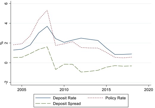
Average deposit spreads in Norway

This figure plots Norwegian policy rates (https://www.norges-bank.no/en/topics/Monetary-policy/Policy-rate/), average deposit rates taken from www.finansportalen.no/, and their difference by year.

Open in new tab Download slide

1 Contributions to the Existing Literature

Our paper relates to at least three strands of the literature: (1) the benefits of issuing deposits for banks, (2) the role of switching costs and inaction in relationship banking, and (3) the broader literature on cross-selling.

First, a rich literature has emphasized the benefits of deposits for banks. Drechsler, Savov, and Schnabl (2017) emphasize that deposits are a cheap and stable financing source for lending. Berlin and Mester (1999) and Drechsler, Savov, and Schnabl (2021) stress that deposit interest rates have a low sensitivity to market interest rates and hence allow banks to take on less interest rate risk. Li, Loutskina, and Strahan (2023) in turn point out that deposits are associated with limited liquidity risk. Beyond these benefits of deposits as a source to refinance lending, Mester (1987), Kashyap, Rajan, and Stein (2002), Gatev, Schuermann, and Strahan (2009), or Robles-Garcia, Benetton, and Buchak (2022) emphasize different synergies from issuing deposits together with offering other bank services, such as lending, for instance, by using the same branches, staff, IT, or other resources. Our paper contributes to this literature by documenting and exploring a new channel of how deposits add value for banks via generating more scope for cross-selling of loans to the same household. Our paper therefore lends support to the view that the activities on the asset and the liability side of banks are related, in contrast to, for instance, the baseline version of the Monti-Klein model (Freixas and Rochet 2008).

Second, a large literature has documented switching costs in banking. One strand of the literature focuses on switching costs within the market for specific products, for instance, U.S. (Sharpe 1997), Finnish (Shy 2002), Spanish (Carbo-Valverde, Hannan, and Rodriguez-Fernandez 2011), or Dutch (Deuflhard 2018) deposit markets, or U.S. (Kim, Kliger, and Vale 2003) or European (Liaudinskas and Grigaite 2021) loan markets. Another strand of this literature focuses on the relationship aspect of switching costs and the role of asymmetric information. Petersen and Rajan (1994) and Mester, Nakamura, and Renault (2007) are seminal papers in this literature, both focusing on bank-firm relationships where much lending is uncollateralized and creditworthiness is often harder to evaluate than for the average household. These studies emphasize the value of a bank’s prior knowledge of the client in facilitating screening. Our paper contributes to this literature by documenting and exploring the drivers of switching costs in bank-household relationships.

Third, several studies explore the importance and determinants of cross-selling. Li, Sun, and Montgomery (2011) and Li, Sun, and Wilcox (2005) posit a theory of how institutions can improve profits from cross-selling. Gupta et al. (2006) compute customer lifetime value (CLV) as net present value from each customer and discuss different models to estimate for each client the optimal acquisition cost in order to optimize profits from the sum of acquisition, retention and cross-selling. They focus on acquisition via marketing, we focus on product pricing. Implications of client stickiness also have been explored in the industrial organization literature (see, e.g., Tirole 1988 or Klemperer 1995). An emerging literature focuses on cross-selling in banking. Hellmann, Lindsey, and Puri (2008), Laux and Walz (2009), Ivashina and Kovner (2011), Carbo-Valverde, Hannan, and Rodriguez-Fernandez (2011), Lepetit et al. (2008), Agarwal et al. (2018), Neuhann and Saidi (2018), Qi (2017), Norden and Weber (2010), and Santikian (2014) focus on either bank-level indications of cross-selling or the cross-selling of products by banks to firms. A common thread of many of these papers is the driving factor supply complementarities. We contribute to this literature with evidence on cross-selling to households. In contrast to the literature on bank-firm relationships, we show that demand complementarities are an important determinant of cross-selling to households, thus contributing to market power and bank franchise values.²

2 Data and Summary Statistics

In this section we describe the main data sources, the measurement of key variables and provide and discuss some summary statistics of the variables most relevant to our analysis.

2.1 Data sources

We use data from four sources in the analysis.

2.1.1 Deposit and loans accounts

The first data source is relationship-level data from the Norwegian tax register covering all outstanding loan and deposit relationships between Norwegian individuals and Norwegian banks.³ These data contain information on the amount deposited at or borrowed from a given bank, in addition to the observed interest paid or received over the year. The data are annual, reported at the end of the year and covers the period 2004–2018. The data are high-quality and third-party reported by banks and other institutions. These data—in addition to the data source discussed next—have been obtained by the Tax Authorities for tax purposes. Norway levies a wealth tax on households, and as such the Tax Authorities are enabled a detailed overview of the balance sheet of each Norwegian household, including deposit and loan information. Most of the loans in our data are mortgages, and most deposit accounts have either a short fixed term or an indefinite term. At an aggregate level, 85% of household credit in Norway are mortgages (Baltzersen 2020). More than 99% of outstanding deposits have a maturity of less than a year.

2.1.2 Other household information

The second data source is a comprehensive overview of individual-level information for all Norwegian taxpayers. This information includes a detailed breakdown of individuals’ balance sheets, containing information on (among other things) income sources, assets, and liabilities. It also contains information about demographics, including age, education, and location. These annual data are reported at the end of the year and cover the years 2004–2018.

2.1.3 Bank-level information

We add bank-level information from the supervisory database ORBOF, which covers all major balance sheet and income statement items for the universe of banks operating in Norway.

2.1.4 Finansportalen.no

The fourth and final data source is daily interest rates at the product level from the price comparison website Finansportalen.no. Since 2008, all banks have been obliged by law to report each day the interest rate on their outstanding deposit products, as well as different contractual terms, such as volume limits and age restrictions.

2.1.5 Combining the data

Our primary data for analysis consists of merged data from the three first data sources. The fourth data set is used for supplementary analysis. We aggregate our data to the bank-household-year level, as major financial decisions like mortgage borrowing are often decided at the household level. So the unit of observation in our data is a bank-household-year triplet.

When analyzing depositor borrower conversion, that is, the propensity for household h to take out a loan with bank b in year t conditional on having had deposits there in prior years, we do not count deposit accounts opened in the year in which the loan is initiated. By dropping those (small number of) cases, we may slightly underestimate the positive effect of a deposit relationship on starting another relationship with the same bank. Still, we wish to avoid artificial inflation of the importance of the relationship by counting deposit accounts opened as the bank required the household to do so in connection with a loan.

2.2 Variable definitions and summary statistics

Most of the variables we use in our analysis are relatively straightforward, that is, loan and deposit volumes. However, some key variables are constructed based on the raw data. Below, we will outline how we construct these variables.

2.2.1 Deposit and loan rates

To impute deposit (loan) rates, we divide the interest a household receives (pays) from (to) a bank in a given year by the deposits (debt) it holds there. We compute debt and deposits as the average between the outstanding balances in years t – 1 and t.⁴ We then compute loan spreads as the imputed loan rate less the policy rate, and deposit spreads as the policy rate less the imputed deposit rate.

2.2.2 Education characteristics

We bin households into different groups of different variables to ensure comparability between households. For most variables, for instance, labor income, we bin based on the household’s position in the distribution (i.e., first, second, third, and fourth quartiles). For education, however, we bin them into four groups based on absolute education levels: (1) those with at most elementary education, (2) those with elementary + high school, (3) those with a bachelor’s degree (undergraduate level), and (4) those with a master’s degree or higher (graduate level).

2.2.3 Market power metrics

As we observe the universe of Norwegian deposit and loan balances, we can also compute each bank’s market share for each of deposit and loan products in each municipality.⁵ We compute market shares, Herfindahl-Hirschmann indices (HHI) for both loans and deposits within each municipality, as well as banks’ weighted HHIs as the weighted average of the HHIs in the municipalities the banks operate in, weighted with their exposures to these areas.

2.2.4 Summary statistics

In Table 1, panel A, we provide summary statistics on the bank-household-year triplets underlying most of our analyses. To start with, we see that the policy rate varies between 0.50% and 5.32% and averaged 1.82% in our sample. Imputed deposit rates vary between 0.07% and 4.92%, which implies deposit spreads of between –2.84 and 4.76, with an average of 0.54 pp. Loan rates range between 1.23% and 9.01% and an average 3.59%, which results in raw loan spreads of between 3.12% and 7.19%, with an average of 1.54%. Average deposit volumes correspond to NOK 140,000, or roughly about US$14,000 or 14,000 euro, while loan volumes average NOK 160,000 and in the last observed relationship year NOK 1.1 million. Household debt to all banks used by that household across all years observed is on average NOK 970,000. Deposit interest lost from failing to switch banks averages 2.4 pp, or 320,000 NOK p.a., when comparing the interest households actually earn to the highest rate earned by anyone in the same municipality and year including accounts not everyone is eligible for. The duration of bank relationships we observe ranges from 1 to 15 years and averages close to 9 years.

Table 1

Open in new tab

Summary statistics

	Observations	Mean	SD	Min	Max
A. Relationship characteristics
Policy rate (pp)	46,132,510	1.82	1.23	0.50	5.32
Deposit rate (pp)	46,132,510	1.29	1.18	0.07	4.92
Deposit spread (pp)	46,132,510	0.54	1.37	–2.84	4.76
Loan rate (pp)	11,883,905	3.59	1.66	1.23	9.01
Loan spread (pp)	11,883,905	1.54	1.65	–3.12	7.19
Mean deposit volume (NOK)	46,132,510	140,000	300,000	0	2,000,000
Mean loan volume (NOK)	46,132,510	160,000	510,000	0	4,000,000
Final loan volume (NOK)	46,132,510	1,100,000	1,500,000	0	6,900,000
Mean household debt (NOK)	46,132,510	970,000	1,300,000	0	6,900,000
Deposit interest lost (pp)	46,132,510	2.40	1.22	–3.06	4.82
Deposit money lost (NOK)	46,132,510	320,000	480,000	0	1,800,000
Relationship duration (years)	46,132,510	8.91	4.26	1.00	15.00
B. Household characteristics
I(Age < 30)	46,132,510	.34	.47	.00	1.00
I(Education group 1)	45,754,686	.15	.35	.00	1.00
I(Education group 2)	45,754,686	.42	.49	.00	1.00
I(Education group 3)	45,754,686	.30	.46	.00	1.00
I(Education group 4)	45,754,686	.13	.34	.00	1.00
I(Has real estate)	46,132,510	.53	.50	.00	1.00
House value (NOK)	46,132,510	1,200,000	1,900,000	–5,000,000	440,000,000
HH’s # of banks	46,132,510	2.88	1.60	1.00	7.00
Population density	12,918,625	1.00	0.87	0.00	2.40
C. Bank and market characteristics
Conversion	46,132,508	3.41	2.52	0.00	8.93
Bank deposits (NOK mio)	46,132,510	86,000	110,000	0	310,000
HHI(D)	46,132,510	.30	.12	.11	.86
HHI(L)	46,132,510	.18	.09	.08	.86
WHHI(D)	46,132,510	.30	.07	.13	.69
WHHI(L)	46,132,510	.18	.05	.00	.49
WMS(D)	46,132,510	.31	.16	.00	.69
WMS(L)	46,132,510	.16	.10	.00	.52

	Observations	Mean	SD	Min	Max
A. Relationship characteristics
Policy rate (pp)	46,132,510	1.82	1.23	0.50	5.32
Deposit rate (pp)	46,132,510	1.29	1.18	0.07	4.92
Deposit spread (pp)	46,132,510	0.54	1.37	–2.84	4.76
Loan rate (pp)	11,883,905	3.59	1.66	1.23	9.01
Loan spread (pp)	11,883,905	1.54	1.65	–3.12	7.19
Mean deposit volume (NOK)	46,132,510	140,000	300,000	0	2,000,000
Mean loan volume (NOK)	46,132,510	160,000	510,000	0	4,000,000
Final loan volume (NOK)	46,132,510	1,100,000	1,500,000	0	6,900,000
Mean household debt (NOK)	46,132,510	970,000	1,300,000	0	6,900,000
Deposit interest lost (pp)	46,132,510	2.40	1.22	–3.06	4.82
Deposit money lost (NOK)	46,132,510	320,000	480,000	0	1,800,000
Relationship duration (years)	46,132,510	8.91	4.26	1.00	15.00
B. Household characteristics
I(Age < 30)	46,132,510	.34	.47	.00	1.00
I(Education group 1)	45,754,686	.15	.35	.00	1.00
I(Education group 2)	45,754,686	.42	.49	.00	1.00
I(Education group 3)	45,754,686	.30	.46	.00	1.00
I(Education group 4)	45,754,686	.13	.34	.00	1.00
I(Has real estate)	46,132,510	.53	.50	.00	1.00
House value (NOK)	46,132,510	1,200,000	1,900,000	–5,000,000	440,000,000
HH’s # of banks	46,132,510	2.88	1.60	1.00	7.00
Population density	12,918,625	1.00	0.87	0.00	2.40
C. Bank and market characteristics
Conversion	46,132,508	3.41	2.52	0.00	8.93
Bank deposits (NOK mio)	46,132,510	86,000	110,000	0	310,000
HHI(D)	46,132,510	.30	.12	.11	.86
HHI(L)	46,132,510	.18	.09	.08	.86
WHHI(D)	46,132,510	.30	.07	.13	.69
WHHI(L)	46,132,510	.18	.05	.00	.49
WMS(D)	46,132,510	.31	.16	.00	.69
WMS(L)	46,132,510	.16	.10	.00	.52

Panel A shows household bank relationship characteristics. Rates and spreads (against the policy rate) are expressed in percentage points (pp), volumes in Norwegian Kroners (NOK). Panel B shows household characteristics, mostly with indicators denoted as I. Panel C shows bank and municipal market characteristics. There HHI(D) and HHI(L) stand for the household municipality’s Herfindahl-Hirschmann index (HHI) for the deposit (D) and loan (L) market, respectively. WHHI(D) and WHHI(L) stand for the corresponding bank-level values, weighted by the bank’s portfolios across municipalities, while WMS stand for each bank’s weighted market share. The conversion variable summarizes the bank-level means of each relationship’s mean loan over mean deposit volume.

Table 1

Open in new tab

Summary statistics

	Observations	Mean	SD	Min	Max
A. Relationship characteristics
Policy rate (pp)	46,132,510	1.82	1.23	0.50	5.32
Deposit rate (pp)	46,132,510	1.29	1.18	0.07	4.92
Deposit spread (pp)	46,132,510	0.54	1.37	–2.84	4.76
Loan rate (pp)	11,883,905	3.59	1.66	1.23	9.01
Loan spread (pp)	11,883,905	1.54	1.65	–3.12	7.19
Mean deposit volume (NOK)	46,132,510	140,000	300,000	0	2,000,000
Mean loan volume (NOK)	46,132,510	160,000	510,000	0	4,000,000
Final loan volume (NOK)	46,132,510	1,100,000	1,500,000	0	6,900,000
Mean household debt (NOK)	46,132,510	970,000	1,300,000	0	6,900,000
Deposit interest lost (pp)	46,132,510	2.40	1.22	–3.06	4.82
Deposit money lost (NOK)	46,132,510	320,000	480,000	0	1,800,000
Relationship duration (years)	46,132,510	8.91	4.26	1.00	15.00
B. Household characteristics
I(Age < 30)	46,132,510	.34	.47	.00	1.00
I(Education group 1)	45,754,686	.15	.35	.00	1.00
I(Education group 2)	45,754,686	.42	.49	.00	1.00
I(Education group 3)	45,754,686	.30	.46	.00	1.00
I(Education group 4)	45,754,686	.13	.34	.00	1.00
I(Has real estate)	46,132,510	.53	.50	.00	1.00
House value (NOK)	46,132,510	1,200,000	1,900,000	–5,000,000	440,000,000
HH’s # of banks	46,132,510	2.88	1.60	1.00	7.00
Population density	12,918,625	1.00	0.87	0.00	2.40
C. Bank and market characteristics
Conversion	46,132,508	3.41	2.52	0.00	8.93
Bank deposits (NOK mio)	46,132,510	86,000	110,000	0	310,000
HHI(D)	46,132,510	.30	.12	.11	.86
HHI(L)	46,132,510	.18	.09	.08	.86
WHHI(D)	46,132,510	.30	.07	.13	.69
WHHI(L)	46,132,510	.18	.05	.00	.49
WMS(D)	46,132,510	.31	.16	.00	.69
WMS(L)	46,132,510	.16	.10	.00	.52

	Observations	Mean	SD	Min	Max
A. Relationship characteristics
Policy rate (pp)	46,132,510	1.82	1.23	0.50	5.32
Deposit rate (pp)	46,132,510	1.29	1.18	0.07	4.92
Deposit spread (pp)	46,132,510	0.54	1.37	–2.84	4.76
Loan rate (pp)	11,883,905	3.59	1.66	1.23	9.01
Loan spread (pp)	11,883,905	1.54	1.65	–3.12	7.19
Mean deposit volume (NOK)	46,132,510	140,000	300,000	0	2,000,000
Mean loan volume (NOK)	46,132,510	160,000	510,000	0	4,000,000
Final loan volume (NOK)	46,132,510	1,100,000	1,500,000	0	6,900,000
Mean household debt (NOK)	46,132,510	970,000	1,300,000	0	6,900,000
Deposit interest lost (pp)	46,132,510	2.40	1.22	–3.06	4.82
Deposit money lost (NOK)	46,132,510	320,000	480,000	0	1,800,000
Relationship duration (years)	46,132,510	8.91	4.26	1.00	15.00
B. Household characteristics
I(Age < 30)	46,132,510	.34	.47	.00	1.00
I(Education group 1)	45,754,686	.15	.35	.00	1.00
I(Education group 2)	45,754,686	.42	.49	.00	1.00
I(Education group 3)	45,754,686	.30	.46	.00	1.00
I(Education group 4)	45,754,686	.13	.34	.00	1.00
I(Has real estate)	46,132,510	.53	.50	.00	1.00
House value (NOK)	46,132,510	1,200,000	1,900,000	–5,000,000	440,000,000
HH’s # of banks	46,132,510	2.88	1.60	1.00	7.00
Population density	12,918,625	1.00	0.87	0.00	2.40
C. Bank and market characteristics
Conversion	46,132,508	3.41	2.52	0.00	8.93
Bank deposits (NOK mio)	46,132,510	86,000	110,000	0	310,000
HHI(D)	46,132,510	.30	.12	.11	.86
HHI(L)	46,132,510	.18	.09	.08	.86
WHHI(D)	46,132,510	.30	.07	.13	.69
WHHI(L)	46,132,510	.18	.05	.00	.49
WMS(D)	46,132,510	.31	.16	.00	.69
WMS(L)	46,132,510	.16	.10	.00	.52

In panel B, we report household characteristics independent of a particular bank relationship. We see that 34% of households have at least one member below 30 years old when we first observe their bank relationship.⁶ In addition, 15% fall into education group 1, 42% into group 2, 30% into group 3, and 13% into group 4, where the different education groups correspond as discussed above to elementary school, high school, undergraduate, or graduate level, respectively. In the relationship years when we observe them, about 53% of households have nonzero taxable real estate, which the tax authorities value on average (including zeros) at NOK 1.2 million. Households use between 1 and 7 banks and on average 3 banks. The mean population density is 1,000 capita per km².

Finally, in panel C, we report key bank and municipal market characteristics. To start with, we find that the average bank converts in its average relationship each NOK of deposits into 3.4 NOK of loan volume. In terms of bank size, we see the average bank holding about NOK 86 billion deposits. Municipal deposit (loan) markets have Herfindahl-Hirschmann indices (HHI) of market concentration of, on average, 0.3 (0.18). Bank-level-weighted HHI values differ from bank to bank, but their averages are the same as the municipal ones. Finally, banks have average portfolio-weighted deposit (loan) market shares of 31% (16%).

3 Cross-Selling of Deposits and Loans

In this section, we explore whether banks cross-sell future deposit accounts or loans to existing depositors. We start by documenting substantial inaction in bank-household deposit relationships, which is also conditional on proxies for households’ outside options. We then document that existing depositors are substantially more likely to be converted to future borrowers, compared to other households with similar characteristics.

3.1 Cross-selling of deposits

3.1.1 Empirical strategy

To investigate the presence of cross-selling of future deposit accounts, we compare the likelihood that a depositor h at bank b at time t will also have a relationship with that bank in a subsequent period

t + τ

compared to the alternatives that either the household has no more deposits at all or holds all deposits only with any of the other banks present in the municipality that household h resides.⁷ Specifically, we regress the indicator

I {(Existing Depositor)}_{h, b, t + τ})

for an existing deposit relationship between household h and bank b at time

t + τ

on the indicator

I {(Depositor)}_{h, b, t}

because there is such a relationship in t. We absorb the highest available rate in the area and hence a reasonable proxy for households outside options through municipality × year fixed effects. Specifically, we estimate

I {(Depositor)}_{h, b, t + τ} = α + β * I {(ExistingDepositor)}_{h, b, t} + δ_{m, t} + ε_{h, t} .

(1)

The key coefficient is β, which captures the persistence in the bank-household deposit relationship. As almost all deposit accounts in Norway and hence in our data are either indefinite term contracts or fixed term for a very limited amount of time, this coefficient captures persistence in bank-household deposit relationships due to households choosing to stay with bank b.⁸

Next, we will explore whether the costs of any potential inaction vary with household characteristics by computing explicitly the difference between the deposit rate in that relationship and the top deposit rate paid by any other bank in that municipality and year. We multiply this difference for each relationship with the average deposit amount held to obtain also interest income lost in NOK. This is a rough approximation as the top deposit rate may often be restricted to accounts with limited eligibility, as discussed below. We denote this interest income lost as

Y_{h, b, t}

⁠. We then relate this to household characteristics

X_{h}

⁠:

Los s_{h, b, t} = α + β * X_{h, t} + ε_{h, b, t} .

(2)

3.1.2 Empirical results on cross-selling of deposits

Figure 3 shows results related to the cross-selling of deposits. In the year after we first observe household h to hold deposits at bank b, the household is still a bit over 90-pp more likely to hold deposits at bank b than at any other randomly chosen bank that also offers deposit accounts in the same municipality, even after controlling for outside options.⁹ This persistence gradually declines each year after we first observe a deposit relationship, but even after the maximum observed time period of 14 years it still exceeds 50 pp.

Fig. 3

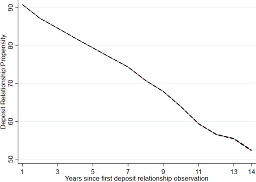
Depositor stickiness

Estimates are obtained using a data set where for each household × year we fill in also all other banks present in that municipality and which the household could alternatively have been using. Then we control for municipality × year fixed effects to capture all outside options.

Open in new tab Download slide

Table 2 reports results on the determinants of this inaction, where we measure the extent of inaction as the loss of income from continuing the existing bank relationship instead of switching to another bank available in that municipality. This variable, in a parsimonious way, captures the monetary costs of inaction. Columns 1 and 3 explore the determinants of the deposit rate lost, that is, in the difference between the approximated deposit rate earned in the observed relationship and the best one paid in any other relationship in that municipality and year. In columns 2 and 4 the outcome of interest is the log of deposit income lost. In columns 1 and 2 we regress the outcomes of interest only on household observables, whereas in columns 3 and 4 we condition also on municipality × salary quarter × education group fixed effects. Overall, the fixed effects turn out to make only a limited difference, so we focus on the latter two columns, which we deem more conservative.

Table 2

Open in new tab

Determinants of deposits lost by not switching banks

	(1)	(2)	(3)	(4)
	Deposit rate lost	log deposit income lost	Deposit rate lost	log deposit income lost
I(Parent)	–0.180***	–0.143***	–0.148***	–0.216***
	(0.001)	(0.002)	(0.001)	(0.002)
I(Retired)	–0.063***	0.724***	–0.096***	0.704***
	(0.001)	(0.001)	(0.001)	(0.002)
ln(Inc)	0.018***	–0.076***	0.022***	–0.090***
	(0.000)	(0.001)	(0.000)	(0.001)
ln(Wealth)	–0.047***	0.304***	–0.041***	0.295***
	(0.000)	(0.000)	(0.000)	(0.000)
ln(Deposits)	0.004***	0.019***	0.005***	0.019***
	(0.000)	(0.000)	(0.000)	(0.000)
I(Age <30)	–0.264***	0.142***	–0.277***	0.188***
	(0.001)	(0.001)	(0.001)	(0.001)
Constant	2.871***	7.908***	2.764***	8.188***
	(0.003)	(0.007)	(0.003)	(0.008)
Observations	46,134,493	44,257,652	45,756,649	43,888,934
R ²	.019	.181	.039	.198
Fixed effects	N	N	Y	Y

	(1)	(2)	(3)	(4)
	Deposit rate lost	log deposit income lost	Deposit rate lost	log deposit income lost
I(Parent)	–0.180***	–0.143***	–0.148***	–0.216***
	(0.001)	(0.002)	(0.001)	(0.002)
I(Retired)	–0.063***	0.724***	–0.096***	0.704***
	(0.001)	(0.001)	(0.001)	(0.002)
ln(Inc)	0.018***	–0.076***	0.022***	–0.090***
	(0.000)	(0.001)	(0.000)	(0.001)
ln(Wealth)	–0.047***	0.304***	–0.041***	0.295***
	(0.000)	(0.000)	(0.000)	(0.000)
ln(Deposits)	0.004***	0.019***	0.005***	0.019***
	(0.000)	(0.000)	(0.000)	(0.000)
I(Age <30)	–0.264***	0.142***	–0.277***	0.188***
	(0.001)	(0.001)	(0.001)	(0.001)
Constant	2.871***	7.908***	2.764***	8.188***
	(0.003)	(0.007)	(0.003)	(0.008)
Observations	46,134,493	44,257,652	45,756,649	43,888,934
R ²	.019	.181	.039	.198
Fixed effects	N	N	Y	Y

The deposit rate lost for each relationship × year is the difference between the maximum rate paid by any bank in that year and municipality and the rate earned in that relationship and year. The deposit income lost is computed as the product of that rate loss and the deposit volume in each relationship and year. We then regress the rate lost and log income lost on client observables. Columns 3 and 4 include additionally fixed effects for each combination of municipality, salary quarter, and education group. Standard errors clustered by relationship are in parentheses.

p < .1;

p < .05;

***

p < .01.

Table 2

Open in new tab

Determinants of deposits lost by not switching banks

	(1)	(2)	(3)	(4)
	Deposit rate lost	log deposit income lost	Deposit rate lost	log deposit income lost
I(Parent)	–0.180***	–0.143***	–0.148***	–0.216***
	(0.001)	(0.002)	(0.001)	(0.002)
I(Retired)	–0.063***	0.724***	–0.096***	0.704***
	(0.001)	(0.001)	(0.001)	(0.002)
ln(Inc)	0.018***	–0.076***	0.022***	–0.090***
	(0.000)	(0.001)	(0.000)	(0.001)
ln(Wealth)	–0.047***	0.304***	–0.041***	0.295***
	(0.000)	(0.000)	(0.000)	(0.000)
ln(Deposits)	0.004***	0.019***	0.005***	0.019***
	(0.000)	(0.000)	(0.000)	(0.000)
I(Age <30)	–0.264***	0.142***	–0.277***	0.188***
	(0.001)	(0.001)	(0.001)	(0.001)
Constant	2.871***	7.908***	2.764***	8.188***
	(0.003)	(0.007)	(0.003)	(0.008)
Observations	46,134,493	44,257,652	45,756,649	43,888,934
R ²	.019	.181	.039	.198
Fixed effects	N	N	Y	Y

	(1)	(2)	(3)	(4)
	Deposit rate lost	log deposit income lost	Deposit rate lost	log deposit income lost
I(Parent)	–0.180***	–0.143***	–0.148***	–0.216***
	(0.001)	(0.002)	(0.001)	(0.002)
I(Retired)	–0.063***	0.724***	–0.096***	0.704***
	(0.001)	(0.001)	(0.001)	(0.002)
ln(Inc)	0.018***	–0.076***	0.022***	–0.090***
	(0.000)	(0.001)	(0.000)	(0.001)
ln(Wealth)	–0.047***	0.304***	–0.041***	0.295***
	(0.000)	(0.000)	(0.000)	(0.000)
ln(Deposits)	0.004***	0.019***	0.005***	0.019***
	(0.000)	(0.000)	(0.000)	(0.000)
I(Age <30)	–0.264***	0.142***	–0.277***	0.188***
	(0.001)	(0.001)	(0.001)	(0.001)
Constant	2.871***	7.908***	2.764***	8.188***
	(0.003)	(0.007)	(0.003)	(0.008)
Observations	46,134,493	44,257,652	45,756,649	43,888,934
R ²	.019	.181	.039	.198
Fixed effects	N	N	Y	Y

p < .1;

p < .05;

***

p < .01.

The results indicate that deposit rate or income lost due to inaction varies with household characteristics. Households in which the household head is less than 30 years old lose 28-bp less deposit rate and 18% less deposit income, while parents lose 15 bp and 23% less, respectively. These two characteristics are plausibly correlated with both higher price sensitivity and lower switching costs, which are more likely to increase with age and bank relationship duration. Retiree status and wealth are associated with smaller losses in terms of the interest rate but bigger losses in terms of deposit income, presumably as these two groups are on average also reasonably price sensitive but have greater deposit volumes at stake. These results are largely consistent with those of Andersen et al. (2020), who document that wealth and age are important determinants of switching cost related to psychological and information gathering costs.

3.2 Cross-selling of loans

3.2.1 Empirical strategy

Practitioner accounts suggest that banks strive to sell different types of products to the same client over time.¹⁰ One reason for this to be attractive is that the same kind of switching costs that lead households to keep their deposits with the same bank may also lead them to apply for a loan to that same bank. In this case, we have demand complementarities. These complementarities can be due to efforts to align bank incentives as in Laux and Walz (2009), due to physical switching costs as in Sharpe (1997), administrative and cognitive costs (Handel 2013; Andersen et al. 2020) or due to loyalty as in Ongena, Paraschiv, and Reite (2021). Motivated by this literature, we investigate whether existing depositors have an elevated propensity to become a borrower at their relationship bank. We exploit the granularity of our data to ensure that we compare fairly similar households. To remove the concern of reverse causality, we focus on loan relationships that started at least 1 year after the client established the deposit account.¹¹

A concern with this analysis is that the deposit and loan relationships may be driven by a third factor. For example, a household and a bank that are present in a municipality with few other banks may be more likely to have a deposit and a loan relationship simply because few alternatives are available. To account for that, we use municipality fixed effects and focus on within-municipality variation, comparing later borrowing between a current depositor to someone not currently depositing with that bank but who lives in the same municipality. Relatedly, loans—most of which are mortgages—may be more likely in a specific phase of the life cycle where households also change depositor status. We, therefore, also partition households into age groups and compare within municipality × age groups. Finally, we consider also the case that the propensity to open a deposit account now, possibly even at a particularly advantageous rate, and the propensity to buy a house later are also driven by the same unobservable personality trait or education. Therefore, we interact the product of municipality and age group fixed effects with salary group and education group fixed effects. To conclude, we regress an indicator I for a loan to household h from bank b in years

τ = 1, \dots, 14

on an indicator for a deposit relationship between h and b in year t:

I {(Borrower)}_{h, b, t + τ} = α + β * I {(ExistingDepositor)}_{h, b, t} + δ_{m, a, s, e} + ε_{h, b, t} .

(3)

Although $I {(Loan)}_{h, b, t + τ}$ is a binary outcome, our baseline analysis uses a linear probability model (LPM) to make it computationally feasible to include our highly granular fixed effects and so compare a household with deposits at bank b to one that has its deposits elsewhere but is otherwise as much as possible comparable to the former household.

3.2.2 Empirical results on cross-selling of loans

Figure 4 visually displays the results from estimating Equation (3). The existence of a deposit relationship in year t increases the likelihood of observing a new loan between the bank and that household with roughly 4 pp in $t + 1$ ⁠. The marginal effect is still a bit over 2 pp after 2 years, and then gradually falls year by year but remains statistically significant and positive throughout the full sample up to 14 years for which we observe bank-household relationships. As an alternative reference, year-by-year estimates are displayed also Internet Appendix Table 1. Cumulatively these marginal effects make an existing depositor close to 20-pp more likely to borrow from its deposit-taking than an observationally similar household with no deposits at that bank.¹² Overall, this suggests significant effects of an existing deposit relationship on the likelihood of a loan relationship which banks may want to consider also when onboarding and retaining depositors.

Fig. 4

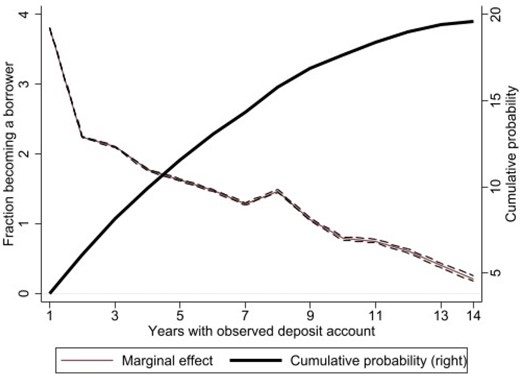
Existing depositors and subsequent borrowing

This figure plots our estimates of the marginal and cumulative effect of a household’s opening of a deposit account with a bank on the propensity for that household to borrow from that bank in each of the subsequent 14 years, along with 95% confidence intervals. The sample includes also hypothetical relations of each household with any other bank present in the municipality. Regressions control for municipality × salary group × education × age group fixed effects.

Open in new tab Download slide

3.2.3 Robustness

In Internet Appendix Table 2, panel A we show further evidence on the impact of existing deposit relationships on the propensity to borrow. In the top panel, we compare the effects of using different estimation approaches to estimating the effect of a deposit relationship in any observed year on the propensity to start a loan one year later. Linear probability model (LPM) estimations without any fixed effects yield an effect of 2.2 pp, logit estimations yield marginal effects of 2.4, and probit estimations of 2.3 pp. Adding the full set of fixed effects reduces the estimate to 2.1 pp. This suggests that using a LPM with fixed effects is, if anything, slightly more conservative, but does not differ significantly from the discussed alternatives.

While panel A starts from actually observed bank-household relationships only, panel B fills in for each household also all potential relationships with all banks that have at least one relationship in the household’s municipality. Doing so increases the sample size by about 28%. The estimates increase from 2.1 to 2.3 pp when using fixed effects or from 2.2 to 2.7 pp when not using fixed effects. The difference is not large. This fits with the observation from Table 1 that the average household uses already close to 3 banks and a maximum of 7, reflecting that municipalities have a limited number of banks.

In both samples without and with hypothetical relationships of each household with each other bank active in that municipality, we find a strong link between deposit and loan relationships, and this is not significantly weakened by any of our fixed effects. This suggests that the results are not driven by unobservables. Yet one still may be concerned that both relationships are driven by the geographical distance between a household’s exact address and the address of its bank’s closest branch, neither of which we can observe beyond the postcode. We explore this in Internet Appendix Tables 3–7 and show that our results are robust to focusing on a subsample of movers (both within and across municipalities), markets with a high population density, and markets with low banking concentration. We will explain these tests in more detail in Section 5.1.1.

Table 3

Open in new tab

Loan pricing

	(1)	(2)	(3)	(4)	(5)	(6)
	Loan rate	Loan spread	Loan rate	Loan spread	Loan rate	Loan spread
I(Depositor)	0.147***	0.146***	0.226***	0.223***	0.267***	0.265***
	(0.037)	(0.036)	(0.027)	(0.026)	(0.026)	(0.025)
ln(Debt)			–0.124***	–0.122***	–0.124***	–0.122***
			(0.004)	(0.004)	(0.005)	(0.004)
I(Owns real estate)			–0.320***	–0.314***
			(0.026)	(0.025)
ln(Deposits)			0.001**	0.001**	0.001***	0.001***
			(0.001)	(0.001)	(0.001)	(0.001)
Birth year			–0.005***	–0.005***	–0.005***	–0.005***
			(0.000)	(0.000)	(0.000)	(0.000)
Has ever received UI			0.053***	0.052***	0.045***	0.045***
			(0.002)	(0.002)	(0.002)	(0.002)
Number of banks used			–0.102***	–0.100***	–0.092***	–0.090***
			(0.005)	(0.005)	(0.005)	(0.005)
ln(House value)					–0.098***	–0.096***
					(0.006)	(0.006)
Constant	3.377***	1.528***	15.212***	13.420***	16.345***	14.525***
	(0.021)	(0.020)	(0.530)	(0.524)	(0.597)	(0.591)
Observations	19,990,561	19,990,561	5,196,287	5,196,287	4,601,525	4,601,525
R ²	.158	.222	.237	.297	.279	.304
Bank × Year FE	Y	Y	Y	Y	Y	Y
Municipality × Education
× Year FE	N	N	Y	Y	Y	Y

	(1)	(2)	(3)	(4)	(5)	(6)
	Loan rate	Loan spread	Loan rate	Loan spread	Loan rate	Loan spread
I(Depositor)	0.147***	0.146***	0.226***	0.223***	0.267***	0.265***
	(0.037)	(0.036)	(0.027)	(0.026)	(0.026)	(0.025)
ln(Debt)			–0.124***	–0.122***	–0.124***	–0.122***
			(0.004)	(0.004)	(0.005)	(0.004)
I(Owns real estate)			–0.320***	–0.314***
			(0.026)	(0.025)
ln(Deposits)			0.001**	0.001**	0.001***	0.001***
			(0.001)	(0.001)	(0.001)	(0.001)
Birth year			–0.005***	–0.005***	–0.005***	–0.005***
			(0.000)	(0.000)	(0.000)	(0.000)
Has ever received UI			0.053***	0.052***	0.045***	0.045***
			(0.002)	(0.002)	(0.002)	(0.002)
Number of banks used			–0.102***	–0.100***	–0.092***	–0.090***
			(0.005)	(0.005)	(0.005)	(0.005)
ln(House value)					–0.098***	–0.096***
					(0.006)	(0.006)
Constant	3.377***	1.528***	15.212***	13.420***	16.345***	14.525***
	(0.021)	(0.020)	(0.530)	(0.524)	(0.597)	(0.591)
Observations	19,990,561	19,990,561	5,196,287	5,196,287	4,601,525	4,601,525
R ²	.158	.222	.237	.297	.279	.304
Bank × Year FE	Y	Y	Y	Y	Y	Y
Municipality × Education
× Year FE	N	N	Y	Y	Y	Y

Columns 1, 3, and 5 use as outcome the loan rate. Columns 2, 4, and 6 the spread thereof over the policy rate. See the main text for the rationale. “I” stands for indicators; “ln” for natural logarithms; and “UI” for unemployment insurance benefits. Standard errors clustered by bank × year are in parentheses.

p < .1;

p < .05;

***

p < .01.

Table 3

Open in new tab

Loan pricing

	(1)	(2)	(3)	(4)	(5)	(6)
	Loan rate	Loan spread	Loan rate	Loan spread	Loan rate	Loan spread
I(Depositor)	0.147***	0.146***	0.226***	0.223***	0.267***	0.265***
	(0.037)	(0.036)	(0.027)	(0.026)	(0.026)	(0.025)
ln(Debt)			–0.124***	–0.122***	–0.124***	–0.122***
			(0.004)	(0.004)	(0.005)	(0.004)
I(Owns real estate)			–0.320***	–0.314***
			(0.026)	(0.025)
ln(Deposits)			0.001**	0.001**	0.001***	0.001***
			(0.001)	(0.001)	(0.001)	(0.001)
Birth year			–0.005***	–0.005***	–0.005***	–0.005***
			(0.000)	(0.000)	(0.000)	(0.000)
Has ever received UI			0.053***	0.052***	0.045***	0.045***
			(0.002)	(0.002)	(0.002)	(0.002)
Number of banks used			–0.102***	–0.100***	–0.092***	–0.090***
			(0.005)	(0.005)	(0.005)	(0.005)
ln(House value)					–0.098***	–0.096***
					(0.006)	(0.006)
Constant	3.377***	1.528***	15.212***	13.420***	16.345***	14.525***
	(0.021)	(0.020)	(0.530)	(0.524)	(0.597)	(0.591)
Observations	19,990,561	19,990,561	5,196,287	5,196,287	4,601,525	4,601,525
R ²	.158	.222	.237	.297	.279	.304
Bank × Year FE	Y	Y	Y	Y	Y	Y
Municipality × Education
× Year FE	N	N	Y	Y	Y	Y

	(1)	(2)	(3)	(4)	(5)	(6)
	Loan rate	Loan spread	Loan rate	Loan spread	Loan rate	Loan spread
I(Depositor)	0.147***	0.146***	0.226***	0.223***	0.267***	0.265***
	(0.037)	(0.036)	(0.027)	(0.026)	(0.026)	(0.025)
ln(Debt)			–0.124***	–0.122***	–0.124***	–0.122***
			(0.004)	(0.004)	(0.005)	(0.004)
I(Owns real estate)			–0.320***	–0.314***
			(0.026)	(0.025)
ln(Deposits)			0.001**	0.001**	0.001***	0.001***
			(0.001)	(0.001)	(0.001)	(0.001)
Birth year			–0.005***	–0.005***	–0.005***	–0.005***
			(0.000)	(0.000)	(0.000)	(0.000)
Has ever received UI			0.053***	0.052***	0.045***	0.045***
			(0.002)	(0.002)	(0.002)	(0.002)
Number of banks used			–0.102***	–0.100***	–0.092***	–0.090***
			(0.005)	(0.005)	(0.005)	(0.005)
ln(House value)					–0.098***	–0.096***
					(0.006)	(0.006)
Constant	3.377***	1.528***	15.212***	13.420***	16.345***	14.525***
	(0.021)	(0.020)	(0.530)	(0.524)	(0.597)	(0.591)
Observations	19,990,561	19,990,561	5,196,287	5,196,287	4,601,525	4,601,525
R ²	.158	.222	.237	.297	.279	.304
Bank × Year FE	Y	Y	Y	Y	Y	Y
Municipality × Education
× Year FE	N	N	Y	Y	Y	Y

p < .1;

p < .05;

***

p < .01.

Table 4

Open in new tab

Screening of future defaulters

	(1)	(2)
	Loan rate	Loan spread
Future default	0.05***	0.05***
	(0.01)	(0.01)
I(Depositor)	0.27***	0.26***
	(0.02)	(0.02)
Future default x I(Depositor)	–0.02	–0.02
	(0.02)	(0.02)
ln(Debt)	–0.12***	–0.12***
	(0.00)	(0.00)
ln(House value)	–0.09***	–0.09***
	(0.01)	(0.01)
ln(Deposits)	0.00***	0.00***
	(0.00)	(0.00)
Birth year	–0.01***	–0.01***
	(0.00)	(0.00)
Has ever received UI	0.04***	0.04***
	(0.00)	(0.00)
Number of banks used	–0.09***	–0.09***
	(0.00)	(0.00)
Constant	17.37***	15.54***
	(0.66)	(0.66)
Observations	5,165,425	5,165,425
R ²	.27	.30
Bank × Year FE	Y	Y
Municipality × Education × Year FE	Y	Y

	(1)	(2)
	Loan rate	Loan spread
Future default	0.05***	0.05***
	(0.01)	(0.01)
I(Depositor)	0.27***	0.26***
	(0.02)	(0.02)
Future default x I(Depositor)	–0.02	–0.02
	(0.02)	(0.02)
ln(Debt)	–0.12***	–0.12***
	(0.00)	(0.00)
ln(House value)	–0.09***	–0.09***
	(0.01)	(0.01)
ln(Deposits)	0.00***	0.00***
	(0.00)	(0.00)
Birth year	–0.01***	–0.01***
	(0.00)	(0.00)
Has ever received UI	0.04***	0.04***
	(0.00)	(0.00)
Number of banks used	–0.09***	–0.09***
	(0.00)	(0.00)
Constant	17.37***	15.54***
	(0.66)	(0.66)
Observations	5,165,425	5,165,425
R ²	.27	.30
Bank × Year FE	Y	Y
Municipality × Education × Year FE	Y	Y

This table shows the results from regressing the loan rate and loan spread on a wide range of household characteristics, including a dummy for whether the household eventually defaults. Default is measured as an event where the outstanding debt is nonzero, but the bank has not received any interest payments. Standard errors clustered by bank × year are in parentheses.

p < .1;

p < .05;

***

p < .01.

Table 4

Open in new tab

Screening of future defaulters

	(1)	(2)
	Loan rate	Loan spread
Future default	0.05***	0.05***
	(0.01)	(0.01)
I(Depositor)	0.27***	0.26***
	(0.02)	(0.02)
Future default x I(Depositor)	–0.02	–0.02
	(0.02)	(0.02)
ln(Debt)	–0.12***	–0.12***
	(0.00)	(0.00)
ln(House value)	–0.09***	–0.09***
	(0.01)	(0.01)
ln(Deposits)	0.00***	0.00***
	(0.00)	(0.00)
Birth year	–0.01***	–0.01***
	(0.00)	(0.00)
Has ever received UI	0.04***	0.04***
	(0.00)	(0.00)
Number of banks used	–0.09***	–0.09***
	(0.00)	(0.00)
Constant	17.37***	15.54***
	(0.66)	(0.66)
Observations	5,165,425	5,165,425
R ²	.27	.30
Bank × Year FE	Y	Y
Municipality × Education × Year FE	Y	Y

	(1)	(2)
	Loan rate	Loan spread
Future default	0.05***	0.05***
	(0.01)	(0.01)
I(Depositor)	0.27***	0.26***
	(0.02)	(0.02)
Future default x I(Depositor)	–0.02	–0.02
	(0.02)	(0.02)
ln(Debt)	–0.12***	–0.12***
	(0.00)	(0.00)
ln(House value)	–0.09***	–0.09***
	(0.01)	(0.01)
ln(Deposits)	0.00***	0.00***
	(0.00)	(0.00)
Birth year	–0.01***	–0.01***
	(0.00)	(0.00)
Has ever received UI	0.04***	0.04***
	(0.00)	(0.00)
Number of banks used	–0.09***	–0.09***
	(0.00)	(0.00)
Constant	17.37***	15.54***
	(0.66)	(0.66)
Observations	5,165,425	5,165,425
R ²	.27	.30
Bank × Year FE	Y	Y
Municipality × Education × Year FE	Y	Y

p < .1;

p < .05;

***

p < .01.

Table 5

Open in new tab

Instrumental variable regressions on depositor-borrower conversion

	(1)	(2)	(3)	(4)	(5)	(6)	(7)	(8)
	I(Future loan)	I(Future loan)	I(Depositor)	I(Future loan)	I(Future loan)	I(Future loan)	I(Depositor)	I(Future loan)
I(Existing depositor)	0.080***			0.205***	0.030***			0.110***
	(0.000)			(0.000)	(0.000)			(0.001)
Old dep market share		0.244***	1.189***			0.019***	0.176***
		(0.000)	(0.000)			(0.000)	(0.000)
Current dep market share					0.205***	0.226***	1.020***	0.114***
					(0.000)	(0.000)	(0.000)	(0.001)
Constant	0.002***	0.001***	0.008***		0.001***	0.001***	0.006***
	(0.000)	(0.000)	(0.000)		(0.000)	(0.000)	(0.000)
Observations	110,640,774	110,640,774	110,640,774	110,640,774	110,640,774	110,640,774	110,640,774	110,640,774
R ²	.067	.080	.223	–.052	.102	.099	.294	.047
Regression	OLS	RF	FS	IV	OLS	RF	FS	IV
Cluster	MAS*E	MAS*E	MAS*E	MAS*E	MAS*E	MAS*E	MAS*E	MAS*E

	(1)	(2)	(3)	(4)	(5)	(6)	(7)	(8)
	I(Future loan)	I(Future loan)	I(Depositor)	I(Future loan)	I(Future loan)	I(Future loan)	I(Depositor)	I(Future loan)
I(Existing depositor)	0.080***			0.205***	0.030***			0.110***
	(0.000)			(0.000)	(0.000)			(0.001)
Old dep market share		0.244***	1.189***			0.019***	0.176***
		(0.000)	(0.000)			(0.000)	(0.000)
Current dep market share					0.205***	0.226***	1.020***	0.114***
					(0.000)	(0.000)	(0.000)	(0.001)
Constant	0.002***	0.001***	0.008***		0.001***	0.001***	0.006***
	(0.000)	(0.000)	(0.000)		(0.000)	(0.000)	(0.000)
Observations	110,640,774	110,640,774	110,640,774	110,640,774	110,640,774	110,640,774	110,640,774	110,640,774
R ²	.067	.080	.223	–.052	.102	.099	.294	.047
Regression	OLS	RF	FS	IV	OLS	RF	FS	IV
Cluster	MAS*E	MAS*E	MAS*E	MAS*E	MAS*E	MAS*E	MAS*E	MAS*E

This table restricts attention to a subsample of movers and shows the results from an IV regression where I(Existing depositor) is instrumented using the market share of the bank in the old municipality. The sample is filled in to include for each household also potential relationships with all banks doing business in that household’s current municipality, as explained in the main text. “RF” corresponds to reduced form, that is, regressing the key dependent variable directly on the instrument, while “FS” corresponds to the first stage. All six columns control for municipality × age group × salary group × education group fixed effects. Columns 1–4 do not, while columns 5–8 do control for the bank’s market share in the household’s current municipality. Standard errors clustered by bank × year are in parentheses.

p < .1;

p < .05;

***

p < .01.

Table 5

Open in new tab

Instrumental variable regressions on depositor-borrower conversion

	(1)	(2)	(3)	(4)	(5)	(6)	(7)	(8)
	I(Future loan)	I(Future loan)	I(Depositor)	I(Future loan)	I(Future loan)	I(Future loan)	I(Depositor)	I(Future loan)
I(Existing depositor)	0.080***			0.205***	0.030***			0.110***
	(0.000)			(0.000)	(0.000)			(0.001)
Old dep market share		0.244***	1.189***			0.019***	0.176***
		(0.000)	(0.000)			(0.000)	(0.000)
Current dep market share					0.205***	0.226***	1.020***	0.114***
					(0.000)	(0.000)	(0.000)	(0.001)
Constant	0.002***	0.001***	0.008***		0.001***	0.001***	0.006***
	(0.000)	(0.000)	(0.000)		(0.000)	(0.000)	(0.000)
Observations	110,640,774	110,640,774	110,640,774	110,640,774	110,640,774	110,640,774	110,640,774	110,640,774
R ²	.067	.080	.223	–.052	.102	.099	.294	.047
Regression	OLS	RF	FS	IV	OLS	RF	FS	IV
Cluster	MAS*E	MAS*E	MAS*E	MAS*E	MAS*E	MAS*E	MAS*E	MAS*E

	(1)	(2)	(3)	(4)	(5)	(6)	(7)	(8)
	I(Future loan)	I(Future loan)	I(Depositor)	I(Future loan)	I(Future loan)	I(Future loan)	I(Depositor)	I(Future loan)
I(Existing depositor)	0.080***			0.205***	0.030***			0.110***
	(0.000)			(0.000)	(0.000)			(0.001)
Old dep market share		0.244***	1.189***			0.019***	0.176***
		(0.000)	(0.000)			(0.000)	(0.000)
Current dep market share					0.205***	0.226***	1.020***	0.114***
					(0.000)	(0.000)	(0.000)	(0.001)
Constant	0.002***	0.001***	0.008***		0.001***	0.001***	0.006***
	(0.000)	(0.000)	(0.000)		(0.000)	(0.000)	(0.000)
Observations	110,640,774	110,640,774	110,640,774	110,640,774	110,640,774	110,640,774	110,640,774	110,640,774
R ²	.067	.080	.223	–.052	.102	.099	.294	.047
Regression	OLS	RF	FS	IV	OLS	RF	FS	IV
Cluster	MAS*E	MAS*E	MAS*E	MAS*E	MAS*E	MAS*E	MAS*E	MAS*E

p < .1;

p < .05;

***

p < .01.

Table 6

Open in new tab

Switching as a function of bank tenure

	(1)	(2)
	Switcher	Switcher
I(Age < 30)	0.069***
	(0.000)
I(Wealth <P50)	0.116***	0.052***
	(0.000)	(0.002)
I(University)	0.021***
	(0.000)
Bank tenure	–0.055***	–0.050***
	(0.000)	(0.001)
Constant	0.395***	0.449***
	(0.001)	(0.003)
Observations	3,307,023	3,258,934
R ²	.298	.357
Municipality × Age ×	N	Y
Salary × Education FE

	(1)	(2)
	Switcher	Switcher
I(Age < 30)	0.069***
	(0.000)
I(Wealth <P50)	0.116***	0.052***
	(0.000)	(0.002)
I(University)	0.021***
	(0.000)
Bank tenure	–0.055***	–0.050***
	(0.000)	(0.001)
Constant	0.395***	0.449***
	(0.001)	(0.003)
Observations	3,307,023	3,258,934
R ²	.298	.357
Municipality × Age ×	N	Y
Salary × Education FE

The sample investigates for all household × year combinations in which a new loan is taken out whether the household did already hold deposits at that bank before (Switcher $= 0$ ⁠; about 75% of cases) or not (Switcher $= 1$ ⁠; about 25% of cases). Standard errors are in parentheses.

p < .1;

p < .05;

***

p < .01.

Table 6

Open in new tab

Switching as a function of bank tenure

	(1)	(2)
	Switcher	Switcher
I(Age < 30)	0.069***
	(0.000)
I(Wealth <P50)	0.116***	0.052***
	(0.000)	(0.002)
I(University)	0.021***
	(0.000)
Bank tenure	–0.055***	–0.050***
	(0.000)	(0.001)
Constant	0.395***	0.449***
	(0.001)	(0.003)
Observations	3,307,023	3,258,934
R ²	.298	.357
Municipality × Age ×	N	Y
Salary × Education FE

	(1)	(2)
	Switcher	Switcher
I(Age < 30)	0.069***
	(0.000)
I(Wealth <P50)	0.116***	0.052***
	(0.000)	(0.002)
I(University)	0.021***
	(0.000)
Bank tenure	–0.055***	–0.050***
	(0.000)	(0.001)
Constant	0.395***	0.449***
	(0.001)	(0.003)
Observations	3,307,023	3,258,934
R ²	.298	.357
Municipality × Age ×	N	Y
Salary × Education FE

p < .1;

p < .05;

***

p < .01.

Table 7

Open in new tab

Household and bank determinants of loan probability, loan amount, and deposit pricing

	(1)	(2)	(3)	(4)	(5)	(6)
	I(Loan)	ln(FinalDebt)	Dspread	I(Loan)	ln(FinalDebt)	Dspread
I(Parent)	–0.022***	0.635***	–0.156***	–0.023***	0.446***	–0.135***
	(0.000)	(0.005)	(0.003)	(0.000)	(0.005)	(0.009)
I(Retired)	0.013***	–2.797***	–0.040***	0.029***	–1.235***	–0.029***
	(0.000)	(0.003)	(0.001)	(0.000)	(0.004)	(0.004)
ln(Inc)	0.008***	0.932***	–0.011***	0.003***	0.590***	–0.016***
	(0.000)	(0.002)	(0.000)	(0.000)	(0.002)	(0.002)
ln(Wealth)	0.001***	0.142***	–0.027***	0.001***	0.086***	–0.027***
	(0.000)	(0.001)	(0.000)	(0.000)	(0.001)	(0.002)
ln(Deposits)	0.003***	–0.062***	–0.005***	0.003***	–0.059***	–0.005***
	(0.000)	(0.000)	(0.000)	(0.000)	(0.000)	(0.001)
I(Age <30)	0.075***	0.999***	–0.258***	0.074***	0.827***	–0.281***
	(0.000)	(0.003)	(0.001)	(0.000)	(0.003)	(0.007)
HH’s # of banks	–0.013***	0.582***	–0.086***	–0.014***	0.478***	–0.078***
	(0.000)	(0.001)	(0.000)	(0.000)	(0.001)	(0.002)
Multiproduct HH			0.086***			0.082***
			(0.001)			(0.010)
Constant	–0.027***	–3.759***	1.608***	–0.007***	1.229***	1.644***
	(0.001)	(0.020)	(0.003)	(0.001)	(0.025)	(0.013)
Observations	17,090,102	17,090,102	7,806,169	16,860,604	16,860,604	7,684,772
R ²	.047	.199	.027	.058	.229	.041
MSE FE	N	N	N	Y	Y	Y
Cluster	Rel	Rel	Rel	MSE	MSE	MSE

	(1)	(2)	(3)	(4)	(5)	(6)
	I(Loan)	ln(FinalDebt)	Dspread	I(Loan)	ln(FinalDebt)	Dspread
I(Parent)	–0.022***	0.635***	–0.156***	–0.023***	0.446***	–0.135***
	(0.000)	(0.005)	(0.003)	(0.000)	(0.005)	(0.009)
I(Retired)	0.013***	–2.797***	–0.040***	0.029***	–1.235***	–0.029***
	(0.000)	(0.003)	(0.001)	(0.000)	(0.004)	(0.004)
ln(Inc)	0.008***	0.932***	–0.011***	0.003***	0.590***	–0.016***
	(0.000)	(0.002)	(0.000)	(0.000)	(0.002)	(0.002)
ln(Wealth)	0.001***	0.142***	–0.027***	0.001***	0.086***	–0.027***
	(0.000)	(0.001)	(0.000)	(0.000)	(0.001)	(0.002)
ln(Deposits)	0.003***	–0.062***	–0.005***	0.003***	–0.059***	–0.005***
	(0.000)	(0.000)	(0.000)	(0.000)	(0.000)	(0.001)
I(Age <30)	0.075***	0.999***	–0.258***	0.074***	0.827***	–0.281***
	(0.000)	(0.003)	(0.001)	(0.000)	(0.003)	(0.007)
HH’s # of banks	–0.013***	0.582***	–0.086***	–0.014***	0.478***	–0.078***
	(0.000)	(0.001)	(0.000)	(0.000)	(0.001)	(0.002)
Multiproduct HH			0.086***			0.082***
			(0.001)			(0.010)
Constant	–0.027***	–3.759***	1.608***	–0.007***	1.229***	1.644***
	(0.001)	(0.020)	(0.003)	(0.001)	(0.025)	(0.013)
Observations	17,090,102	17,090,102	7,806,169	16,860,604	16,860,604	7,684,772
R ²	.047	.199	.027	.058	.229	.041
MSE FE	N	N	N	Y	Y	Y
Cluster	Rel	Rel	Rel	MSE	MSE	MSE

Household characteristics until the indicator for age below 30 as above. HH’s # of banks is the number of banks with which the household entertains a relationship in that year. Multiproduct HH is an indicator for households that have both deposits and a loan in that bank relationship. Columns 1–3 without fixed effects and with standard errors clustered by bank relationship. Columns 4–6 include municipality × salary × education fixed effects and cluster standard errors by these same categories.

p < .1;

p < .05;

***

p < .01.

Table 7

Open in new tab

Household and bank determinants of loan probability, loan amount, and deposit pricing

	(1)	(2)	(3)	(4)	(5)	(6)
	I(Loan)	ln(FinalDebt)	Dspread	I(Loan)	ln(FinalDebt)	Dspread
I(Parent)	–0.022***	0.635***	–0.156***	–0.023***	0.446***	–0.135***
	(0.000)	(0.005)	(0.003)	(0.000)	(0.005)	(0.009)
I(Retired)	0.013***	–2.797***	–0.040***	0.029***	–1.235***	–0.029***
	(0.000)	(0.003)	(0.001)	(0.000)	(0.004)	(0.004)
ln(Inc)	0.008***	0.932***	–0.011***	0.003***	0.590***	–0.016***
	(0.000)	(0.002)	(0.000)	(0.000)	(0.002)	(0.002)
ln(Wealth)	0.001***	0.142***	–0.027***	0.001***	0.086***	–0.027***
	(0.000)	(0.001)	(0.000)	(0.000)	(0.001)	(0.002)
ln(Deposits)	0.003***	–0.062***	–0.005***	0.003***	–0.059***	–0.005***
	(0.000)	(0.000)	(0.000)	(0.000)	(0.000)	(0.001)
I(Age <30)	0.075***	0.999***	–0.258***	0.074***	0.827***	–0.281***
	(0.000)	(0.003)	(0.001)	(0.000)	(0.003)	(0.007)
HH’s # of banks	–0.013***	0.582***	–0.086***	–0.014***	0.478***	–0.078***
	(0.000)	(0.001)	(0.000)	(0.000)	(0.001)	(0.002)
Multiproduct HH			0.086***			0.082***
			(0.001)			(0.010)
Constant	–0.027***	–3.759***	1.608***	–0.007***	1.229***	1.644***
	(0.001)	(0.020)	(0.003)	(0.001)	(0.025)	(0.013)
Observations	17,090,102	17,090,102	7,806,169	16,860,604	16,860,604	7,684,772
R ²	.047	.199	.027	.058	.229	.041
MSE FE	N	N	N	Y	Y	Y
Cluster	Rel	Rel	Rel	MSE	MSE	MSE

	(1)	(2)	(3)	(4)	(5)	(6)
	I(Loan)	ln(FinalDebt)	Dspread	I(Loan)	ln(FinalDebt)	Dspread
I(Parent)	–0.022***	0.635***	–0.156***	–0.023***	0.446***	–0.135***
	(0.000)	(0.005)	(0.003)	(0.000)	(0.005)	(0.009)
I(Retired)	0.013***	–2.797***	–0.040***	0.029***	–1.235***	–0.029***
	(0.000)	(0.003)	(0.001)	(0.000)	(0.004)	(0.004)
ln(Inc)	0.008***	0.932***	–0.011***	0.003***	0.590***	–0.016***
	(0.000)	(0.002)	(0.000)	(0.000)	(0.002)	(0.002)
ln(Wealth)	0.001***	0.142***	–0.027***	0.001***	0.086***	–0.027***
	(0.000)	(0.001)	(0.000)	(0.000)	(0.001)	(0.002)
ln(Deposits)	0.003***	–0.062***	–0.005***	0.003***	–0.059***	–0.005***
	(0.000)	(0.000)	(0.000)	(0.000)	(0.000)	(0.001)
I(Age <30)	0.075***	0.999***	–0.258***	0.074***	0.827***	–0.281***
	(0.000)	(0.003)	(0.001)	(0.000)	(0.003)	(0.007)
HH’s # of banks	–0.013***	0.582***	–0.086***	–0.014***	0.478***	–0.078***
	(0.000)	(0.001)	(0.000)	(0.000)	(0.001)	(0.002)
Multiproduct HH			0.086***			0.082***
			(0.001)			(0.010)
Constant	–0.027***	–3.759***	1.608***	–0.007***	1.229***	1.644***
	(0.001)	(0.020)	(0.003)	(0.001)	(0.025)	(0.013)
Observations	17,090,102	17,090,102	7,806,169	16,860,604	16,860,604	7,684,772
R ²	.047	.199	.027	.058	.229	.041
MSE FE	N	N	N	Y	Y	Y
Cluster	Rel	Rel	Rel	MSE	MSE	MSE

p < .1;

p < .05;

***

p < .01.

4 Understanding the Mechanisms behind Cross-Selling

The results above indicate that banks are able to cross-sell loans to existing depositors. However, the underlying mechanism is unclear. On the one hand, there could be supply complementarities from selling different products to the same client because of, for example, more reliable borrower screening, as emphasized by Petersen and Rajan (1994) or Mester, Nakamura, and Renault (2007). As discussed in the introduction, these forms of complementarities have been documented in the literature on firm-bank relationships. On the other hand, demand complementarities could give rise to household inaction (Andersen et al. 2020; Handel 2013). Such inaction could arise from persistent preferences for particular financial institutions, or from stickiness based on search costs (Abel, Eberly, and Panageas 2007) and/or switching costs. Either way, from the economics of multiproduct pricing,¹³ (e.g., Tirole 1988), it is clear that both demand and supply complementarities can motivate firms to price the initial product below marginal cost for future profits.

The purpose of this section is to shed further light on the underlying mechanism through which cross-selling arises. We start by documenting that cross-selling in our setup seems more likely to be demand driven, and then we explore the drivers of these demand factors.

4.1 Supply versus demand complementarities

4.1.1 Empirical strategy on supply versus demand complementarities

To explore whether supply or demand complementarities dominate on average, we test two hypotheses. First, we investigate whether existing depositors get a discount on their loan rate relative to otherwise comparable households with no deposits at that bank.

That is, we estimate the following equation:

LoanRat e_{h, b, t} = α_{b, t} + δ_{m, e, t} + β I {(ExistingDepositor)}_{b, h, t} + γ X_{h, t} + ε_{h, b, t},

(4)

where

α_{b, t}

captures bank × time fixed effects,

δ_{m, e, t}

captures municipality × education × year fixed effects, and

X_{h, t}

is a vector of household-level controls, including ln(debt), a dummy for whether the household is a real estate owner, birth year, a dummy for whether the household is ever unemployed, population density in the municipality of the household, and the number of bank connections of the household. By controlling for this rich set of household, region and bank characteristics, we hold as best as possible households’ outside options in terms of loan rate offers and approval uncertainty fixed.

Observing such a discount (⁠ $β < 0$ ⁠) is consistent with supply complementarities being the dominant driver of cross-selling, as banks that prefer lending to existing clients due to cheaper or more reliable screening should pass a fraction of these benefits on to those clients.

Second, we separately investigate whether an existing deposit relationship does indeed enable banks to screen borrowers better, in which case we would expect a stronger link between loan rates charged and later realized defaults. Specifically, we tag loans as being in default if the outstanding debt is nonzero, but the interest paid over the course of the year is zero. We then tag households as “defaulters” if they ever default and regress the loan rate or loan spread on the defaulter dummy, a dummy for whether there exists a prior deposit relationship, and their interaction. Specifically, we estimate

\begin{matrix} L oanRat e_{h, b, t} = α_{b, t} + δ_{m, e, t} + β I {(ExistingDepositor)}_{b, h, t} + η I {(Defaulter)}_{h, b} \\ + Γ {(ExistingDepositor)}_{b, h, t} \times {(Defaulter)}_{h, b} + X_{h, t} + ε_{h, b, t} . \end{matrix}

(5)

We interpret $Γ > 0$ as evidence for screening benefits, that is, that banks are better equipped to price future defaults for borrowers that have a preexisting relationship with the bank. We interpret $Γ \leq 0$ as suggesting no screening benefits.

4.1.2 Empirical results on supply versus demand complementarities

Table 3 shows our results on loan pricing. In columns 1, 3, and 5 we use the approximated loan rate as outcome, while 2, 4, and 6 use the loan spread.¹⁴ Columns 1 and 2 show the results when we control for bank x year fixed effects, while 3–6 show the results when we also control for a wider set of controls that are plausibly important for assessing credit risk and hence loan rates/spreads. We find that households with an existing deposit account pay between 15 and 27 bp more, rather than less, on a new loan. Based on the discussion above, this is most consistent with cross-selling being predominantly driven by demand complementarities; that is, it is difficult to rationalize why households would pay a premium on a loan, compared to other, similar households, unless they preferred to remain with their existing bank. These findings are consistent also with recent findings by Ongena, Paraschiv, and Reite (2021), who show that a representative Norwegian bank charges extra for existing relative to new mortgage borrowers, and more so for households who have a personal loan officer and may thus feel more loyal.

In Table 4, we explore whether an existing deposit relationship allows banks to better screen borrowers. Regardless of whether we use as outcome the loan rate or the loan spread, we find that defaulters (as observed ex post) are charged on average 5 bp more for their loans ex ante, consistent with risk-based pricing. As in the previous table, we also show that existing depositors on average pay a premium compared to other similar households. Interestingly, however, the risk premium charged to future defaulters does not differ between existing and new clients. In fact, if anything it is 2 bp lower for existing clients. These results—combined with those in Table 3—suggest a limited role for supply complementarities. Rather, they suggest that the key driver of the cross-selling loans to household is demand complementarities.

4.2 Understanding the Sources of Demand Complementarities

4.2.1 Empirical strategy

Demand complementarities can arise through several channels. Below, we explore the relevance of two such channels: stickiness and unobserved persistent preferences.

To distinguish between persistent preferences and stickiness, we adopt three approaches. First, we adopt an instrumental variable approach in which we focus on variation in deposit relationships. Specifically, we restrict attention to municipality movers and run an IV exercise where we use the market shares of banks in the old municipality as an instrument for whether the household has an existing deposit relationship with that bank.¹⁵ We then investigate whether this instrumented existing depositor dummy is significantly associated with the propensity to borrow from that bank also in the year following the move. That is, we run a regression where the second stage is

I {(Borrower)}_{h, b, t + 1} = α + β * I {(\hat{ExistingDepositor})}_{h, b, t} + γ m, a, s, e + ϵ_{h, b, t}

(6)

and where the first-stage is given by

I {(ExistingDepositor)}_{h, b, t} = γ_{0} + γ_{1} M arket shar e_{b, \bar{\bar{m}} (h), t - 1} + η_{h, b, t},

(7)

where

\bar{\bar{m}} (h)

refers to the premove municipality of household h, and

Market shar e_{b, \bar{\bar{m}} (h), t - 1}

is the deposit market share of bank b in the premove municipality of household h. In the set of controls

γ_{m, a, s, e}

⁠, we also include the current deposit market share of bank b. This IV approach captures variation in whether a household is an existing depositor with a given bank driven by bank availability rather than unobserved persistent preferences.

Second, we investigate whether the likelihood of switching banks for borrowing depends on tenure length with the existing bank. That is, we define a borrowing household as a switcher if it borrows from a bank which it did not have a previous deposit relationship with, and a nonswitcher if it borrows from its existing bank. We then investigate whether the switching propensity depends on household characteristics and the duration of the relationship between the household and the bank. Specifically, we estimate

Switche r_{h, b, t} = α + β * Tenur e_{h, b, t} + γ_{m, a, s, e} + ε_{h, b, t}

(8)

and focus our attention on the sign of β. We hypothesize that longer tenure likely will be associated with using more products by the same bank and with having become more accustomed to that bank’s branch location, staff, online banking environment, and other factors (Klemperer 1995).

Third, we refer to the factors that Andersen et al. (2020) found to explain delays in financially beneficial refinancing of mortgages. Specifically, they show that households are inactive because of a mixture of psychological and information gathering costs. Based on their estimated results, psychological costs are increasing in wealth, while information gathering costs are largest for low-educated and low wealth households. We regress a dummy for whether an existing depositor becomes a future borrower on a wide range of household characteristics capturing these aspects and link our findings to these established determinants of switching costs.

4.2.2 Empirical results on the sources of demand complementarities

We start in Table 5 by reporting the results from the IV exercise in which we (a) condition on a sample of movers and (b) instrument the existing depositor dummy with the market share of the bank in the old municipality. In columns 5 to 8, we control also for the market share of the bank in the current municipality. We see that the first stage is strong (columns 3 and 7): a 1-pp increase in the market share of a bank in the old municipality increases the likelihood that the household is an existing depositor by between 0.2 and 1.2 pp. This first-stage effect is highly statistically significant, and the implied F statistic is well above commonly recommended minimum levels.

Columns 4 and 8 report the IV estimates, which are large and highly significant: an existing depositor, instrumented with the market share of the bank in the old municipality, has an increased borrowing probability of 11–20 pp compared to other, similar households. These estimates are larger than the OLS estimates (columns 1 and 5) and suggest that the strong link between being a depositor and becoming a lender at the same bank is not driven by persistent preferences alone but holds also when we focus on variation in prior deposit relationships driven by availability alone.

In Table 6 we then provide an additional test between persistent preferences and stickiness. Specifically, we check whether inaction increases with a household’s bank tenure, in which case it would seem more likely to stem from switching costs, or whether it is tenure-invariant, in which case it would more likely seem to stem from persistent preferences. We start from the subsample of all bank-household relationships that ever take up a new loan and use as outcome an indicator for whether the household is a “switcher” in the sense of starting a new bank relationship with this loan or whether it is a nonswitcher in the sense of borrowing from a bank the household already had a deposit relationship with. Most importantly, we relate this indicator, which takes a value of one in about 25% of cases, to the observed length of the bank-household relationship. This variable, ranging from 1 to 15 years and averaging close to 9 years in our sample is slightly downward-biased due to left-censoring, yet it captures variation in tenure length.

In column 1 we control for and cluster standard errors by relationship fixed effects, while in column 2 we control for and cluster by municipality × age group × salary group × education group fixed effects. Both columns show that the propensity to switch banks when taking out a new loan decreases by at least 5 pp for each year of bank tenure. This provides additional evidence in support of switching costs as the key driver of the observed household inaction.

In Table 7, columns 1 and 4, additionally relate conversion probabilities to household characteristics. We find that old households, wealthier households, and households with fewer prior bank relationships are more likely to convert. These results are largely consistent with switching costs being driven by a mixture between psychological and information gathering costs (Andersen et al. 2020). It is also consistent with the marketing literature which documents how cross-selling potential depends on household characteristics (Li, Sun, and Montgomery 2011; Li, Sun, and Wilcox 2005).

All in all, these results suggest that the observed cross-selling of loans to existing household depositors is driven by demand complementarities compared to supply complementarities, and these in turn seem driven more by stickiness than by unobserved persistent preferences. Next, we will explore the implications of cross-selling for deposit pricing.

5 Deposit Pricing with Cross-Selling

In this section we explore the implications of cross-selling for deposit pricing. We start by focusing on whether cross-selling strategies can explain cross-sectional variation in deposit rates. We then discuss whether they can explain also time-series variation in average deposit rates.

5.1 Implications for deposit pricing in the cross-section

Having documented the potential for cross-selling of future deposits and loans, we now investigate whether banks internalize these cross-selling opportunities when pricing new deposits.

To see why it is profitable for banks to internalize the likelihood of cross-selling, we note that our summary statistics in Table 1 show the average loan amount in our sample to be about NOK 20,000, or US$2,000, higher than the average deposit amount. At the same time, an average deposit spread of 54 bp compares to an average loan spread of 154 bp. As 95% of Norwegian loans are floating rate (IMF 2012), the policy rate seems a sensible benchmark. Moreover, most household loans are collateralized with real estate and banks have historically never had substantial losses on mortgages in our setup (Kragh-Sørensen and Solheim 2014). It therefore seems reasonable to assume a negligible credit risk premium. These facts, together with the fact that about one in five depositors brings in extra loan business in the future, suggest that the profits from cross-selling of future loans is nonnegligible and hence something that banks may want to internalize when setting deposit rates, as already implied by the discussions in Klemperer (1995) and Farrell and Klemperer (2007).

To investigate to what extent banks offer more attractive deposit rates to clients who, in expectation, will bring in more loan profits later, we reduce our panel to a cross-section covering only the first year of each relationship we observe. We then regress an indicator for later borrowing, the log loan amount and the initial deposit spread, all captured by

Y_{h, b}

in Equation (E9), on relevant household characteristics, while controlling for a conservative set of fixed effects:¹⁶

Y_{h, b} = α + β X_{h} + δ_{m, s, e} + ε_{h, b} .

(9)

The household characteristics of interest include a parenthood indicator, a retirement indicator, an indicator for being below 30 years old in the first relationship year, as well as the logs of household income, household wealth, and the relationship-level deposit volume, respectively. We also include each household’s total number of bank relationships in that year. In the deposit spread column, we additionally have an indicator for whether the household is already a “multiproduct” household in the sense of using both the bank’s deposit and the bank’s loan business. To assess its impact, deposit pricing regressions do, in contrast to the conversion regressions discussed above, include a limited number of cases in which a household has a loan from a bank already in or before the year in which we first observe a deposit account.

Table 7, columns 1 and 4, investigates the determinants of whether a current depositor will later also borrow from the same bank, whereas columns 2 and 5 explore those of the expected loan amount, and Columns (3) and (6) those of the initial deposit spread. While columns 1–3 investigate only the determinants explicitly displayed and cluster standard errors by bank relationship, columns 4–6 control additionally for municipality-salary-education group fixed effects and cluster standard errors by these. Overall, the results are qualitatively similar but tend to be slightly smaller when adding the full battery of fixed effects. We deem the latter version more conservative and focus our discussion on that.

The table illustrates large variation in the potential for cross-selling across household characteristics. Column 1 illustrates that parents are ceteris paribus 2.2-pp less likely to borrow than nonparents. However, column 2 then shows the average parent to borrow in expectation about 64% more than the average nonparent. Relatedly, we find those younger than 30 at the observed relationship start to exhibit a 7.4-pp higher borrowing propensity and to borrow a full 83% more in expectation. Life cycle considerations plausibly drive this: those under 30 are likely to buy or refinance their first home.

Having noted that parenthood and age are key predictors of future borrowing, the estimates in column 6 are consistent with banks internalizing this when setting interest rates: parents get, on average, 14-bp lower deposit spreads, while those below 30 get an additional discount of, on average, 28 bp. We note that these associations are driven not by client-specific deposit rates but by each bank and year offering several different deposit products with different rates and eligibility criteria, as Figure 5 with rate data from the price comparison website Finansportalen illustrates. That figure shows, in particular, significantly lower deposit spreads on deposit products explicitly targeted at those below 30 years old. This is consistent with more attractive deposit offers to clients expected to bring in more follow-on business.¹⁷ Beyond banks using account eligibility criteria to price discriminate, different effective rates may come about by households’ differential tendency to reoptimize accounts or banks.

Fig. 5

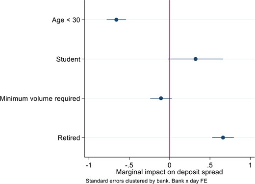
Deposit spreads by account type

Coefficients from regressing deposit spreads on different account types, based on data from Finansportalen.

Open in new tab Download slide

5.1.1 Robustness

The Internet Appendix contains a comprehensive set of robustness checks on those in Table 3 of the main text, which we will briefly discuss here. To start with, a natural question is whether the impact of client observables like parenthood on later borrowing from the observed bank operates primarily through whether the household borrows at all or whether it borrows from that specific bank. Internet Appendix Table 3 explores this by focusing on the subset of relationships by households that become borrowers in the 14 years we study. The key results are similar to those in Table 3.

While the distinction between debtors and no debtors is only about the channel of the effect of an existing deposit on a new loan relationship, a more serious concern is that both could be driven by proximity to the closest bank branches. Although both our year-by-year conversion estimates in Figure 4 and the cross-sectional estimations in Table 3 contain inter alia municipality fixed effects and thereby control for population and bank branch density, we may imagine that within the same municipality, each household is more likely to do business with that bank that offers the branch closest to the household’s place of residence. To investigate this, we exploit that—as visualized in Figure 6—about half of all households move either within or even across municipalities between opening their deposit account and between taking out a loan. On these grounds, Internet Appendix Table 4 focuses on those bank-household relationships where the household moves postcodes¹⁸ between the year when we first see the household to have deposits with that bank and the year in which we first see the household borrow there. While some coefficients become slightly larger and others slightly smaller than in the twice as big baseline sample, none changes significantly. This refutes the potential concern that our results are driven by branch distance. The same holds when in Internet Appendix Table 5, we reduce the sample further to focus only on households who move across municipalities.

Fig. 6

Fraction of bank relationships started before a move

This figure considers for all new debt a household owes to a bank which fraction of households have already moved to a different postcode area within or across municipalities since starting to deposit at that bank.

Open in new tab Download slide

An alternative robustness check focuses on municipalities with high population density and typically higher bank branch density. Internet Appendix Table 6 focuses on households in municipalities with above-median density. As these tend to be larger municipalities with more households, this still includes about 14 million of the initial 17 million observations. Again, we can summarize this robustness check as confirming our baseline estimates. The same holds true when Internet Appendix Table 7 focuses on municipalities with submedian concentration.

5.2 Implications for deposit pricing across the policy rate cycle

We discussed above how banks may want to accept lower deposit spreads in return for higher cross-selling profits. As illustrated in Figure 4, some of this future cross-selling profit may arise only quite a few years after the first observation of the deposit relationship. For instance, many households may start a deposit relationship before their first job and borrow to buy their first home only in or after their first year with significant income of their own. For banks’ optimization, however, this means that they need to discount the benefits of onboarding or retaining a potential future borrower.

Given that future cross-selling profits should be discounted, the level and path of interest rates might affect the extent to which banks internalize cross-selling opportunities when setting deposit rates today. Specifically, when rates are high, future cross-selling opportunities are discounted more and therefore less relevant from the bank’s perspective when computing the expected profitability of a depositor. As a result, future cross-selling potential should matter less for deposit prices today if rates today are high, or expected to be high in the near future.¹⁹

Figure 7 presents in the top panel a binned scatterplot of deposit spreads against nominal policy rates; that is, it plots the “deposit spread β” (Drechsler, Savov, and Schnabl 2017). The clear upward-sloping relationship in the figure suggests that deposit spreads respond less to policy rates when rates are low to begin with. To quantify the magnitude of the relationship, we regress the deposit spread on the policy rate. As highlighted by column 1 of Table 8, we find a β of 0.67, which is similar to the mean β of 0.54 reported for the United States in Drechsler, Savov, and Schnabl (2017). The positive relationship between the policy rate and the deposit spread holds for inflation-adjusted rates or policy rate changes.²⁰

Fig. 7

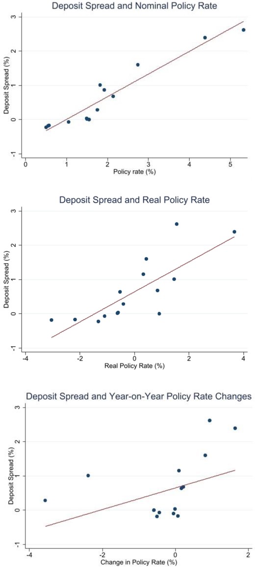
The deposit spread beta

The top panel plots deposit spreads against Norwegian nominal policy rates, the intermediate one against real policy rates (nominal rates less CPI inflation), the bottom panel against year-on-year changes in nominal policy rates.

Open in new tab Download slide

Table 8

Open in new tab

The deposit spread beta by predicted loan propensity and market concentration

	(1)	(2)	(3)	(4)	(5)	(6)	(7)
	Dspread	Dspread	Dspread	Dspread	Dspread	Dspread	Dspread
Policy rate (PR)	0.671***	0.662***	0.649***	0.649***	0.605***	0.670***	0.589***
	(0.000)	(0.000)	(0.000)	(0.000)	(0.000)	(0.000)	(0.000)
I(Conc > P50)		–0.052***	–0.065***	–0.235***	–0.142***	0.080***	0.066***
		(0.001)	(0.001)	(0.001)	(0.001)	(0.001)	(0.001)
PRI(Conc > P50)*		–0.011***	0.016***	0.023***	0.096***	–0.020***	0.063***
		(0.000)	(0.000)	(0.000)	(0.000)	(0.000)	(0.000)
I(PredLoan > P50)		–0.089***	–0.091***	–0.109***	–0.095***	–0.072***	–0.081***
		(0.001)	(0.001)	(0.001)	(0.001)	(0.001)	(0.001)
PRI(PredLoan > P50)*		0.045***	0.049***	0.053***	0.054***	0.044***	0.054***
		(0.000)	(0.000)	(0.000)	(0.000)	(0.000)	(0.000)
Constant	–0.689***	–0.630***	–0.629***	–0.530***	–0.605***	–0.720***	–0.662***
	(0.000)	(0.001)	(0.001)	(0.001)	(0.001)	(0.001)	(0.001)
Observations	45,756,653	45,756,653	45,756,653	45,756,653	45,756,653	45,756,653	45,756,653
R ²	.383	.384	.383	.388	.385	.383	.387
MC measure	None	HHI(D)	HHI(L)	WHHI(D)	WHHI(L)	WMS(D)	WMS(L)

	(1)	(2)	(3)	(4)	(5)	(6)	(7)
	Dspread	Dspread	Dspread	Dspread	Dspread	Dspread	Dspread
Policy rate (PR)	0.671***	0.662***	0.649***	0.649***	0.605***	0.670***	0.589***
	(0.000)	(0.000)	(0.000)	(0.000)	(0.000)	(0.000)	(0.000)
I(Conc > P50)		–0.052***	–0.065***	–0.235***	–0.142***	0.080***	0.066***
		(0.001)	(0.001)	(0.001)	(0.001)	(0.001)	(0.001)
PRI(Conc > P50)*		–0.011***	0.016***	0.023***	0.096***	–0.020***	0.063***
		(0.000)	(0.000)	(0.000)	(0.000)	(0.000)	(0.000)
I(PredLoan > P50)		–0.089***	–0.091***	–0.109***	–0.095***	–0.072***	–0.081***
		(0.001)	(0.001)	(0.001)	(0.001)	(0.001)	(0.001)
PRI(PredLoan > P50)*		0.045***	0.049***	0.053***	0.054***	0.044***	0.054***
		(0.000)	(0.000)	(0.000)	(0.000)	(0.000)	(0.000)
Constant	–0.689***	–0.630***	–0.629***	–0.530***	–0.605***	–0.720***	–0.662***
	(0.000)	(0.001)	(0.001)	(0.001)	(0.001)	(0.001)	(0.001)
Observations	45,756,653	45,756,653	45,756,653	45,756,653	45,756,653	45,756,653	45,756,653
R ²	.383	.384	.383	.388	.385	.383	.387
MC measure	None	HHI(D)	HHI(L)	WHHI(D)	WHHI(L)	WMS(D)	WMS(L)

Dspread is the deposit spread between the policy rate and the deposit rate by bank household relationship and year. We regress it first on the Norwegian central bank’s policy rate (PR) to approximate changes in the discount rates to be applied to future cross-selling profits. The next regressor is I(Conc > P50), an indicator for market concentration above the sample median. Market concentration (MC) is measured as the municipal deposit market Herfindahl-Hirschmann index (HHI) in column 2, the municipal loan market HHI in column 3, the bank-level-weighted deposit (loan) market HHI in column 4 (5), and the bank-level-weighted deposit (loan) market share in column 6 (7). The other indicator of interest is I(PredLoan > P50), which denotes bank-household relationships for whom borrowing propensities predicted by the regressions in Table 4 are above the median. After the PR and the two indicators just described come the regressors of most interest in this table, the interactions between the PR and the two indicators, respectively. All columns control for age group × salary group × education group fixed effects. Standard errors clustered by relationship are in parentheses.

p < .1;

p < .05;

***

p < .01.

Table 8

Open in new tab

The deposit spread beta by predicted loan propensity and market concentration

	(1)	(2)	(3)	(4)	(5)	(6)	(7)
	Dspread	Dspread	Dspread	Dspread	Dspread	Dspread	Dspread
Policy rate (PR)	0.671***	0.662***	0.649***	0.649***	0.605***	0.670***	0.589***
	(0.000)	(0.000)	(0.000)	(0.000)	(0.000)	(0.000)	(0.000)
I(Conc > P50)		–0.052***	–0.065***	–0.235***	–0.142***	0.080***	0.066***
		(0.001)	(0.001)	(0.001)	(0.001)	(0.001)	(0.001)
PRI(Conc > P50)*		–0.011***	0.016***	0.023***	0.096***	–0.020***	0.063***
		(0.000)	(0.000)	(0.000)	(0.000)	(0.000)	(0.000)
I(PredLoan > P50)		–0.089***	–0.091***	–0.109***	–0.095***	–0.072***	–0.081***
		(0.001)	(0.001)	(0.001)	(0.001)	(0.001)	(0.001)
PRI(PredLoan > P50)*		0.045***	0.049***	0.053***	0.054***	0.044***	0.054***
		(0.000)	(0.000)	(0.000)	(0.000)	(0.000)	(0.000)
Constant	–0.689***	–0.630***	–0.629***	–0.530***	–0.605***	–0.720***	–0.662***
	(0.000)	(0.001)	(0.001)	(0.001)	(0.001)	(0.001)	(0.001)
Observations	45,756,653	45,756,653	45,756,653	45,756,653	45,756,653	45,756,653	45,756,653
R ²	.383	.384	.383	.388	.385	.383	.387
MC measure	None	HHI(D)	HHI(L)	WHHI(D)	WHHI(L)	WMS(D)	WMS(L)

	(1)	(2)	(3)	(4)	(5)	(6)	(7)
	Dspread	Dspread	Dspread	Dspread	Dspread	Dspread	Dspread
Policy rate (PR)	0.671***	0.662***	0.649***	0.649***	0.605***	0.670***	0.589***
	(0.000)	(0.000)	(0.000)	(0.000)	(0.000)	(0.000)	(0.000)
I(Conc > P50)		–0.052***	–0.065***	–0.235***	–0.142***	0.080***	0.066***
		(0.001)	(0.001)	(0.001)	(0.001)	(0.001)	(0.001)
PRI(Conc > P50)*		–0.011***	0.016***	0.023***	0.096***	–0.020***	0.063***
		(0.000)	(0.000)	(0.000)	(0.000)	(0.000)	(0.000)
I(PredLoan > P50)		–0.089***	–0.091***	–0.109***	–0.095***	–0.072***	–0.081***
		(0.001)	(0.001)	(0.001)	(0.001)	(0.001)	(0.001)
PRI(PredLoan > P50)*		0.045***	0.049***	0.053***	0.054***	0.044***	0.054***
		(0.000)	(0.000)	(0.000)	(0.000)	(0.000)	(0.000)
Constant	–0.689***	–0.630***	–0.629***	–0.530***	–0.605***	–0.720***	–0.662***
	(0.000)	(0.001)	(0.001)	(0.001)	(0.001)	(0.001)	(0.001)
Observations	45,756,653	45,756,653	45,756,653	45,756,653	45,756,653	45,756,653	45,756,653
R ²	.383	.384	.383	.388	.385	.383	.387
MC measure	None	HHI(D)	HHI(L)	WHHI(D)	WHHI(L)	WMS(D)	WMS(L)

p < .1;

p < .05;

***

p < .01.

An alternative interpretation, however, is that this relationship is driven by bank market power as in Drechsler, Savov, and Schnabl (2017) and not by the discounting of future cross-selling. We therefore investigate whether the relationship between policy rate and deposit spread is stronger for banks in more concentrated markets as predicted and empirically confirmed by Drechsler, Savov, and Schnabl (2017), and whether cross-selling has an independent impact on the deposit spread β as predicted by our new complementary mechanism.

Table 8, column 1, shows the relationship between deposit spreads and policy rates. In columns 2 and 3, we then add interactions of the policy rate with the municipal-level deposit and loan market concentration, respectively, while columns 4 and 5 use the bank-level equivalents obtained as bank portfolio weighted sums of municipal-level values, and columns 6 and 7 use bank-level-weighted market shares in deposit and loan markets, respectively. Our rationale for using bank-level values in addition to municipal-level values is that Norwegian banks are often thought to set prices at the bank level, rather than at the branch level as many U.S. banks are reported to in Drechsler, Savov, and Schnabl (2017). All six columns simultaneously add the interaction of policy rates with the relationship-level loan probability based on the regressions discussed in Section 4 above. Both for market concentration and for borrowing propensities we use binary measures to make estimates more robust to outliers and comparable to each other in terms of specification. The effect of market concentration on the deposit spread β varies between –2 and close to +10 pp depending on the measure used. While it is in fact negative for some of the deposit market measures, it is significant and positive for all measures of loan market concentration.

When we look next at our relationship-level predictor of cross-selling, we find that higher cross-selling potential increases the deposit spread beta, suggesting that the discounting of future cross-selling profits in each bank-household relationship can make deposit spreads more and so deposit rates less sensitive to policy rates. More research is called for to investigate whether or not this has any implications also for deposit and loan volumes and thereby for monetary policy transmission.

6 Conclusion

In this paper we document and explore cross-selling in bank-household relationships. We show that existing depositors have elevated probabilities of remaining a depositor with the same bank despite more attractive outside options and that they have elevated probabilities of becoming a future borrower. We explore the mechanisms behind this cross-selling, and show results that are most consistent with cross-selling being driven by demand rather than by supply complementarities. This is in contrast to findings in the literature on bank-firm relationships, and we rationalize the difference with the fact that credit risk in household mortgage lending can be assessed more easily by assessing the collateral value, making prior information on the borrower relatively less important than for firm lending. We then show that demand complementarities in turn are most likely driven by switching costs rather than by unobserved persistent preferences for certain bank characteristics. Finally, we show that banks internalize this cross-selling potential when setting deposit rates: households that are more likely to be converted to borrowers are offered better deposit terms, and even more so in times of lower policy and discount rates when future cross-selling profits have a higher net present value.

From a theoretical angle, incentives to set lower prices to gain market share and to set higher prices to harvest it have been identified already in the earlier industrial organization literature on switching costs as surveyed by Klemperer (1995). One challenge for suppliers discussed there is the trade-off between gaining market share and harvesting it when suppliers can set only one price for all clients. The retail banking setup we have studied allows banks to address this in three interesting ways: First, by onboarding through deposits and harvesting at least partly through loans, because the average household will start a bank relationship with deposits and buy their house only later. Second, we show that banks can and do effectively price discriminate in the deposits market by offering deposit accounts with different spreads to clients satisfying different eligibility criteria, most importantly age. Third, banks have arguably even more leeway to price discriminate in mortgage lending because mortgage rates are set at the individual level, rather than at the bank level (Ongena et al. 2021), households are inactive due to search or switching costs (Handel 2013; Andersen et al. 2020), and comparison is further complicated for borrowers by the fact that each household will differ in terms of bank-assessed credit risk. We are not aware of an existing theoretical framework that captures all of these components.

Beyond this contribution to the industrial organization and marketing literatures, this paper elucidates banking with a view where the activities on the asset and liability sides are highly interlinked, even within a given client relationship. Our results may have important implications for understanding aspects, such as the zero lower bound on deposit rates and the decline in monetary policy pass-through at low levels (Heider, Saidi, and Schepens 2019; Eggertsson et al. 2019; Basten and Mariathasan 2023). Moreover, it is relevant for understanding the sources of bank market power and franchise values, which have been extensively discussed during recent financial market turmoil. Future research should seek to explore the macroeconomic and financial stability implications of cross-selling in more detail.

We thank, without implicating, the editor Tarun Ramadorai and two very helpful anonymous referees, as well as everyone who provided helpful comments, including Manuel Adelino, Philippe Bacchetta, Allen Berger, Martin Brown, Stefan Bühler, Claudio Calcagno, Santiago Carbo, Giovanni Dell’Arriccia (discussant), Itamar Drechsler, Andreas Fuster, Michel Habib, Mohamed Hamoud, Florian Heider, Stephen Karolyi (discussant), Paul Klemperer, Vardges Levonyan, Lars Norden, Steven Ongena, Per Ostberg, Ana Sa, Joao Santos (discussant), Anthony Saunders, Alexi Savov, Armin Schmutzler, Philipp Schnabl, Johannes Stroebel, and Alexander Wagner, as well as seminar and conference participants at the 21st Annual FDIC Bank Research Conference, ECB, Federal Reserve Board, FINMA, FIRS, IMF, MoFiR, NYU Stern, University of Zurich, SFI Research Days, SNB, Swiss Winter Conference on Financial Intermediation, and WEA-IBEFA. Part of the work on this project was completed while Basten visited NYU Stern and he is very grateful for their hospitality. This paper should not be reported as representing the views of Norges Bank. Supplementary data can be found on The Review of Financial Studies web site.

Footnotes

In Internet Appendix Table 8, we additionally compare conversion propensities across municipalities with proxies for different search costs. These show statistically significant associations with conversion in the expected direction, but economic magnitudes seem limited. We view this as evidence consistent with search costs not being the primary driver of stickiness. But as the proxies are imperfect, we view this last evidence as only tentative.

Kamakura, Ramaswami, and Srivastava (1991) focus on financial services for households and stress that it is often easier to cross-sell to existing customers than to acquire new ones, that customer switching costs (and so presumably the resultant market power) will often increase when a client uses multiple products, and that the typical timing of financial objectives over the life cycle enhances the potential for financial cross-selling, an aspect that will become important when we identify age as one of the key determinants of cross-selling below.

By banks, we mean institutions that are licensed as traditional banks, credit companies (primarily issuing mortgages), or financing companies (primarily issuing unsecured and nonmortgage credit). In an earlier version we also included households’ loan and deposit relationships with institutions without a banking license. Results were similar. Our baseline now focuses on licensed banks to facilitate our interpretation.

While we see deposit volumes and interest by individual or household and bank and year, we unfortunately do not see it by account type and hence cannot sensibly distinguish between “core” and “noncore” deposits.

Many Norwegian municipalities are also physically distant from neighboring ones rather than being contiguous, so treating them as separate local markets seems more appropriate than in more densely populated countries, for example, the Netherlands.

When aggregating from the individual level to the household level, we use birth year and hence the age of the younger spouse, reasoning that one spouse being younger than 30 years old will suffice for access to more attractive deposit accounts.

To ensure that we properly account for all observed and unobserved hypothetical bank-household relationships, we perform this analysis on a data set in which we have filled in hypothetical matches for each household and year with all other banks present in the household’s municipality.

As discussed earlier, less than 1% of deposits had a maturity above 1 year by the end of 2017.

Because of left-censoring in our data, the first year we observe a relationship between a household and a bank may not be the first year of the relationship.

For example, Kane (2005) writes in the practitioner-oriented American Bankers Association Banking Journal: “Since the late 1980s, cross-selling has been the holy grail [italics added] of large banks, particularly in the retail area.”

As in our analyses on the cross-selling of deposits, we complement the data set for these analyses with hypothetical relationships of each household with any other bank also active (as seen at other households) in the same municipality.

Without filling in observations on each household’s hypothetical relationships with other banks in the same municipality, the effect is slightly larger (about 23 pp, as displayed in Internet Appendix Figure 1), but we prefer these more conservative estimates as a baseline.

More specifically in a banking setup, “cross-selling” and the resultant “multiproduct pricing” also may be referred to as “relational banking.” But as the latter may be understood to include borrower monitoring too, we stick to the term “cross-selling.” By contrast, we do not view our setup as one with pure or mixed “bundling,” as discussed by, for example, Cabral and Natividad (2022), wherein a product is sold, respectively, only or at least optionally together with another, as deposit accounts are often opened before a decision on a loan is made. Nor do we deem it feasible for banks to commit to future prices, as in Rochet and Thanassoulis (2019), as they cannot know future policy rates or credit risk distributions.

Given that about 95% of Norwegian mortgages are adjustable rate (IMF 2012), the overnight policy rate seems an acceptable benchmark.

We thank an anonymous referee for this suggestion.

Loan amounts of zero are replaced with 0.01, so that their logarithm exists as well, and hence the outcome can be interpreted as the expected loan amount.

The results are also consistent the explicit suggestion by Carbó Valverde and Rodríguez Fernández (2007) that banks may adopt loss-leader behavior with lower margins on deposits and higher ones on subsequent loans.

We do not see address changes within the same postcode area, but branch distance changes are small.

While we emphasize that banks discount future cross-selling profits less when rates are low a priori, it is also plausible that the depositor borrower conversion is policy rate dependent. It is unclear, however, how the policy rate would affect conversion probabilities. On the one hand, it is plausible to expect ceteris paribus more borrowing and higher conversion when rates are lower. But, on the other hand, policy rate increases typically do not occur ceteris paribus but are instead more likely when the central bank deems credit demand excessive, resulting in an average negative contemporary association between policy rates on the one hand and lending and conversion on the other. To gain a sense of which, if any, of the two mechanisms dominates, we correlated lifetime conversion rates of each relationship with deposit rates in the first relationship year observed. The correlation is close to zero, so for now we focus on rate-dependent discounting of future loan profits rather than rate-dependent loan propensities.

DSS (2017) also analyze the first difference in deposit spreads, but this makes less sense for our relationship-level data as we would then lose a significant portion of observations, and the initial deposit price at onboarding is arguably most interesting.

References

Abel

A. B.

Eberly

J. C.

Panageas

2007

Optimal inattention to the stock market

American Economic Review

244

–

Month:	Total Views:
August 2023	121
September 2023	176
October 2023	193
November 2023	162
December 2023	104
January 2024	177
February 2024	138
March 2024	173
April 2024	183
May 2024	160
June 2024	169
July 2024	170
August 2024	161
September 2024	118
October 2024	198
November 2024	128
December 2024	95
January 2025	140
February 2025	147
March 2025	164
April 2025	172
May 2025	53

Article Contents

Cross-Selling in Bank-Household Relationships: Mechanisms and Implications for Pricing

Abstract

1 Contributions to the Existing Literature

2 Data and Summary Statistics

2.1 Data sources

2.1.1 Deposit and loans accounts

2.1.2 Other household information

2.1.3 Bank-level information

2.1.4 Finansportalen.no

2.1.5 Combining the data

2.2 Variable definitions and summary statistics

2.2.1 Deposit and loan rates

2.2.2 Education characteristics

2.2.3 Market power metrics

2.2.4 Summary statistics

3 Cross-Selling of Deposits and Loans

3.1 Cross-selling of deposits

3.1.1 Empirical strategy

3.1.2 Empirical results on cross-selling of deposits

3.2 Cross-selling of loans

3.2.1 Empirical strategy

3.2.2 Empirical results on cross-selling of loans

3.2.3 Robustness

4 Understanding the Mechanisms behind Cross-Selling

4.1 Supply versus demand complementarities

4.1.1 Empirical strategy on supply versus demand complementarities

4.1.2 Empirical results on supply versus demand complementarities

4.2 Understanding the Sources of Demand Complementarities

4.2.1 Empirical strategy

4.2.2 Empirical results on the sources of demand complementarities

5 Deposit Pricing with Cross-Selling

5.1 Implications for deposit pricing in the cross-section

5.1.1 Robustness

5.2 Implications for deposit pricing across the policy rate cycle

6 Conclusion

Footnotes

References

Supplementary data

Citations

Views

Altmetric

Email alerts

Citing articles via

Latest

Most Read

Most Cited

This Feature Is Available To Subscribers Only