


Abstract
This article shows that individual-level heterogeneity in survival expectations derived from subjective survey information improves the out-of-sample predictions of a dynamic model of retirement and saving. We consider three approaches to modelling survival: life tables, average subjective expectations, and individual-specific estimates based on reported survival probabilities. The models are estimated using Dutch data from the 1990s, a period during which workers could retire from age 59 at no penalty to pension benefits. Actuarial adjustments were introduced in the early 2000s, and we use data from the period 2006–16 to evaluate the accuracy of the counterfactual predictions. While the three models yield different preference estimates, their within-sample fit is similar. Out-of-sample forecasts do differ markedly. The models with homogeneous expectations anticipate a 4- or 5-year increase in the average retirement age in the new regime, compared with an observed increase of 2.6 years. The model with heterogeneous expectations predicts a more realistic increase of 2.7 years. Expectations matter when it comes to counterfactual predictions, even if different combinations of preferences and expectations appear equivalent within a given institutional setting.
1 INTRODUCTION
Life cycle models can be used to understand the drivers of labour supply and saving and to predict the effects of policy changes such as pension reforms. Such models postulate forward-looking agents who base their decisions on expectations as well as preferences (e.g. French, 2005; De Nardi et al., 2010; French and Jones, 2011). This poses an identification problem, since neither preferences nor beliefs are usually directly observed (Manski, 2004). The solution is to pin down expectations using additional information and estimate preferences conditional on those beliefs. Saving, for instance, is determined not only by patience but also by one’s perceived longevity. While survival expectations are typically approximated by actuarial life tables, in this article, we enrich a retirement model with individual-level variation in survival expectations based on probabilities reported by survey respondents. We show that this heterogeneity improves the accuracy of out-of-sample predictions of behaviour after the introduction of actuarial adjustments to pensions.
We formulate a dynamic model of the retirement incentives in the Netherlands during the 1990s. Agents choose their labour supply, benefit claiming, and saving. The model captures all major sources of income (work, pensions, social insurance, and capital income). Future wages, health, and longevity are uncertain. We estimate preference parameters by matching simulations from the model to observed labour supply, benefit claiming, and wealth profiles in the DNB Household Survey (DHS, Centerdata, 1993–2016) and document how expectations affect preference estimates, model fit, and the simulated impact of a large pension reform.
Longevity is modelled according to three methods. The first is the baseline approach that combines actuarial tables with survey data on the likelihood of death conditional on current health. This is the usual way beliefs are handled in empirical life cycle models and neither reflects the average level of subjective expectations nor variation across individuals. The second approach sets the level in accordance with subjective expectations and equates the probability of death with the average subjective probability. The third technique uses reported probabilities to their full potential and introduces individual-level heterogeneity in subjective survival.
Both approaches that utilize subjective beliefs are based on a measurement model which takes into account that probabilities are reported on a coarse 11-point scale. Expectations are assumed to be exogenous and stable, and the incorporation of heterogeneity in subjective survival introduces a single additional state variable in the life cycle model. It has the advantage of relating behaviour to data, rather than increasing flexibility through latent preference types that complicate identification. The method can be applied to other countries and settings, since subjective survival has been elicited in most major household panels (e.g. the HRS in the U.S., SHARE in Europe, and the LISS panel in the Netherlands). The analysis is based on the idea that people act on their expectations, regardless of whether those are reasonable for a given information set. Hence, it is not concerned with the rationality of expectations.
This article fits in the literatures on life cycle models and subjective survival. While longevity risk and detailed descriptions of pension systems have been central to life cycle retirement models since the early 1990s, much progress has been made in the modelling of uncertainty, budgets, and decisions.1 Recent models add uncertainty in wages and unemployment (Gourinchas and Parker, 2002; French, 2005; Low et al., 2010; De Nardi et al., 2020) and in future health and medical expenditures (De Nardi et al., 2010, 2021).2 Moreover, models take into account public and private health insurance (Rust and Phelan, 1997; Van der Klaauw and Wolpin, 2008; De Nardi et al., 2010; French and Jones, 2011) and means-tested government transfers (Hubbard et al., 1994, 1995) to represent household budgets.3 Heyma (2004) analyses Dutch data from the 1990s and shows that it is important to model pensions and social insurance schemes jointly, since they provide alternative pathways into retirement. The literature on subjective survival has established that reported survival probabilities correlate with risk factors in plausible ways and that they predict actual mortality even when controlling for self-reported health (Hamermesh, 1985; Hurd and McGarry, 1995; Hurd et al., 1998; Hurd and McGarry, 2002; Gan et al., 2005).4 Hurd et al. (2004) show that subjective survival predicts retirement and social security claiming in line with life cycle models.
The few studies that use subjective survival in life cycle models mostly assume homogeneous expectations or limit variation to broad groups such as gender and region (e.g. Van der Klaauw and Wolpin, 2008; Haan and Prowse, 2014; Heimer et al., 2019). Li et al. (2014) analyse social security claiming in the U.S. and find that fine-grained actuarial adjustments would motivate those who expect short lives to claim later. Gan et al. (2015) introduce individual-specific subjective survival in a model of saving and show that doing so affects preference estimates, raising risk aversion, and lowering the discount factor.
The article makes four contributions. Firstly, it investigates how individual-specific survival expectations affect labour supply, benefit claiming, and saving while previous work focused only on saving.5 It builds on Gan et al. (2015) in terms of the modelling of expectations: it takes into account measurement error and allows beliefs not to be proportional to life tables (in line with recent evidence, e.g. Wu et al., 2015; Heimer et al., 2019; O’Dea and Sturrock, 2021). Thirdly, this article validates the models by their predictions in a counterfactual policy regime. Such extrapolation is a key application for structural models and provides a strong criterion for model validation, because it limits the scope for data mining (Keane and Wolpin, 2007; Keane, 2010; Keane et al., 2011).6 Two examples that use reforms to validate structural models in the different context of welfare incentives and female labour supply are Keane and Moffitt (1998) and Low et al. (2020).7 To our knowledge, Lumsdaine et al. (1992) is the only paper to apply this validation approach to models of retirement. Fourthly, the institutional context of the Netherlands provides an interesting departure from the U.S. which has been analysed in most previous work. In particular, universal and mandatory pension annuities and health insurance offer more protection against longevity and medical expenditure risk than is common in the U.S.
The results show that estimated preferences and counterfactual predictions strongly depend on survival expectations. In particular, heterogeneous expectations lead to higher risk aversion and a lower and more plausible estimate for the discount factor as in Gan et al. (2015). Moreover, they lower the estimated weight on consumption relative to leisure compared to the two models without variation in expectations. However, within-sample model fit is similar for all three models. Labour supply and pension claiming are matched reasonably well and claiming of disability insurance is reproduced accurately up to the eligibility age for occupational pensions. All wealth quartiles are matched closely up to age bin 70–74, after which confidence intervals for the median and 75th percentile become wide.
Model predictions differ markedly for the counterfactual in which pensions are subject to actuarial adjustments. The data indicate that the average retirement age increased by 2.6 years to 63.8 after early retirement pensions became less generous. This delay in retirement is in line with quasi-experimental evidence of the causal effect of the policy reform (Euwals et al., 2010). However, both models with homogeneous expectations predict a larger increase of 4 or 5 years to a retirement age above 65. The model with variation in survival expectations anticipates a more reasonable increase of 2.7 years to an average retirement age of 63.7. This improvement in accuracy is driven by the estimated parameters for risk aversion, the consumption weight, the discount factor, and the importance of bequests. The estimates obtained under heterogeneous expectations improve counterfactual predictions both overall and conditional on beliefs. Individual-level heterogeneity is key, since counterfactuals for the models with homogeneous expectations are similar despite large differences between life tables and average subjective expectations. These results show that the specification of the mortality process matters for counterfactuals. Heterogeneous expectations derived from subjective data yield more accurate forecasts than homogeneous beliefs, since they better approximate the beliefs that drive behaviour.
The rest of the article is organized as follows. Section 2 describes the life cycle model and the measurement model for subjective survival expectations. The estimation routine is explained in Section 3, after which Section 4 introduces the data. Sections 5–7 present estimation results, model fit, and out-of-sample predictions respectively. Section 9 concludes.
2 MODELS
This section describes the retirement model (Section 2.1) and the measurement model for subjective survival expectations (Section 2.2).
2.1 Retirement model
The model is based on De Bresser et al. (2017). We model the retirement, benefit claiming, and saving decisions of Dutch men aged 50 and older at a yearly resolution. Individuals derive utility from leisure, consumption, and bequests. They face uncertainty in longevity, health, and wages. The model includes public and occupational pensions, which are the most important sources of income in retirement. Unemployment and disability insurance provide alternative exit routes.
We estimate preferences on data from the period 1993–2001, during which early retirement was possible from age 59 on extremely generous terms. In addition to within-sample fit, the model is validated through the accuracy of its predictions for a different policy regime. We use the estimates to simulate the impact of introducing actuarial adjustments to occupational pensions and changing the tax function: the situation in place in the period 2006–16. The following sub-sections explain the model and more information on the institutions is provided in Appendices A and B of the Supplementary Material.
2.1 Decisions
Labour supply and benefit claiming decisions are discrete and consumption is a continuous choice variable. Between the ages (t) of 50 and 69 agents choose one of four levels of labour supply in hours per year: . These levels are set to cover the distribution of hours worked in the sample. We assume that nobody works beyond age 70 in accordance with observed behaviour.8
Figure 1 illustrates the decisions available at all ages. The model includes simplified disability (DI) and unemployment (UI) insurance schemes that provide alternative routes into retirement. UI and DI benefits can be claimed between ages 50 and 64 after which both are replaced by the public pension. Receipt of UI is automatic if the individual does not work or receive DI or occupational pension benefits and is eligible based on his work history (1 year of work translates into 1 month of UI; UI is capped at a maximum of 3 years). The choice to claim DI is restricted to those in poor health, an agent in good health cannot claim DI, and the model does not include an application process or incomplete acceptance. Hence, the evolution of health drives the dynamics of DI claiming. DI is not an absorbing state: agents choose whether to claim each year as long as their health remains poor. This treatment of UI and DI as easily accessible sources of income for pre-retirees is in line with the institutions in place at the time. By the 1990s, the use of these schemes as pathways into retirement was common practice and widely acknowledged and condoned by employers, unions, and the Dutch government (De Jong and Aarts, 1992; Trommel and De Vroom, 1994; Heyma, 2004).
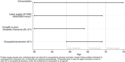
Decisions available at various ages
During the period covered by the analysis, public pension benefits started automatically at age 65. Hence, claiming the public pension is not contingent on any choice made by the agent. While people with entitlements can choose to start claiming occupational pensions at any age between 59 and 69, the 1990s benefit formula incentivizes workers to retire early. In contrast to the DI and UI schemes, claiming occupational pensions is an absorbing state. From age 65 onward those who receive occupational pensions collect both occupational and public pensions. One cannot claim occupational pension, DI or UI benefits and continue to work. As shown in Figure 1, all discrete choices are thus limited to the younger ages. Consumption and hence saving decisions are made until the individual dies (longevity is random and capped at age 100).
Together public and occupational pensions accounted for 94% of retirement income in 2013. The model does not include a decision to switch employers, because most occupational pension funds are organized at the level of broad sectors or industries. Switching employers within such sector does not affect accumulation of entitlements: workers would continue to contribute to the same fund. Similarly, when moving to another sector current entitlements can either be transferred to the new fund or remain dormant in the fund in which they were accumulated. Pension contracts typically do not include a minimum vesting period and do not create incentives for workers to stay put. Therefore, the model allows agents to choose labour supply but abstracts away from the choice of employer.
2.1 Preferences
Individuals derive utility from consumption (), leisure () and, potentially, from bequests. The CRRA utility function is given by
where is an equivalence scale that increases with household size (Scholz et al., 2006). The equivalence scale is the sample average at a given age and does not vary between decision makers (household size and marital status are not state variables in the model).9 Parameter σ determines the concavity of the utility function and thus both risk aversion and the intertemporal elasticity of substitution and κ sets the relative weights of consumption and leisure. Leisure depends on labour supply through the time constraint:
The total time endowment is set to 4,000 hours per year10 and individuals incur a fixed cost ψ when working a positive number of hours. Such fixed cost of work reduces the time budget beyond the hours spent working and raises the marginal value of leisure. Consequently, higher fixed costs induce workers to work fewer hours. Analogously, the time budget is reduced by when in bad health, which increases the marginal value of leisure and rationalizes lower labour supply in poor health. This parameterization of the leisure costs of work and poor health is based on French (2005).
Claiming either UI or DI benefits entails stigma costs, also measured in hours of leisure:
Stigma costs have been proposed as an explanation for low take-up rates of benefits among the eligible population (Moffitt, 1983). Welfare stigma is assumed constant throughout the pre- and post-reform periods, since there has been no major reform to UI or DI and the take-up rates are stable in the sample.
A bequest motive is important to fit saving at older ages. We take the bequest utility function from French (2005) and add one parameter to gain the flexibility required to fit wealth profiles that span the ages 50–84. Previous research based on actual bequests shows that on average widow(-er)s with children do not leave behind larger bequests than those without offspring (Hurd, 1989; Kopczuk and Lupton, 2007). Moreover, De Nardi et al. (2021) find that the desire to leave wealth to the surviving spouse is an important reason for couples to save. In line with those findings, the strength of the bequest motive is allowed to vary with household size through the equivalence scale :
The wealth level is given by and parameters and K govern the importance of bequests and the curvature of bequest utility, respectively.11 allows bequests to weigh more heavily when the equivalence scale is high, that is, at ages at which many spouses are alive.
2.1 Health and wages
While longevity risk is a key driver of behaviour in intertemporal models, agents also face other types of risk. In particular, we allow future health and wages to be uncertain. Since the DHS does not elicit subjective probabilities that measure expectations regarding these variables, we follow the usual approach and assume that agents expect health and wages to develop according to estimated processes.
Health can take two levels: good (2) or bad (1). The probability of being healthy next year is a first-order Markov process that depends on age:
These probabilities are estimated by a logit model which regresses the lead of health on current health and age.
Future wages evolve according to an AR(1) process. While the initial conditions allow for cross-sectional dependence between tenure and wage, the dynamics of wages do not depend on work experience. This is in line with the institutional context of the Netherlands, in which the relation between tenure and salary is fixed through collective labour agreements between employers and employees. In the pre-retirement age range employees are usually at or near the top of the salary ladder for their occupation, which means that additional experience does not affect wages (Ter Weel, 2003; Deelen and Euwals, 2014). Indeed, the data do not indicate that additional experience is associated with changes in wages for the age group 50–64 (estimates from linear fixed effects models available on request). Importantly, simulations indicate that the low longitudinal variation in wages also limits selection issues when estimating the wage process.
2.1 Budget constraint
Cash-on-hand before application of the consumption floor () is equal to:
Here, is the tax function that calculates net income from earnings, DI and UI benefits, public and occupational pensions, and wealth (see Appendix B of the Supplementary Material). Public pensions provide a fixed subsistence income from age 65 onward. Occupational pensions are set as a replacement rate relative to final earnings and thus depend on one’s work history.
Wealth , which is restricted to be non-negative, enters the budget constraint directly and through the tax function, since it generates capital income at a rate of 4% and is taxed at 0.7%.12 The budget constraint also includes an exogenous stream of net income from the spouse given by .13 This does not enter the tax function, because income is taxed at the level of the individual. Finally, out-of-pocket medical expenditures are at the household level. Medical expenditures were of limited importance in the Netherlands during both periods studied in this article and consisted mostly of monthly premiums for mandatory health insurance. Hence, we do not model medical expenditures as an additional source of uncertainty and consider only the mean expenditure by health and age.
Government transfers ensure subsistence expenditures to households whose cash-on-hand drops below a minimum consumption level (Hubbard et al., 1994, 1995):
The minimum consumption level is set to 7,000 euro per year, in line with the income level at which one qualifies for social assistance. Consumption is restricted between zero and .
The model is solved numerically, see Appendix C of the Supplementary Material for more details.
2.1 Policy reform
The Netherlands provides an ideal setting to study the accuracy of out-of-sample predictions of retirement models, because occupational pensions were reformed drastically in 2005. A law in effect from January 1st 2006 places a 52% tax penalty on early retirement pensions for workers born in 1950 or later, effectively prohibiting such schemes. We explain the most important aspects of the pension reform here and refer the reader to Appendices A and B of the Supplementary Material for detailed descriptions of both sets of institutions, including the income tax reform of January 2001.
In the old system occupational pensions, which could not be claimed while working, were divided into two tiers: early retirement pensions (ages 59–64) and regular pensions (ages 65+). The key feature of the system was a strong incentive to retire as early as possible, so that retirees would make place for younger workers. There was no actuarial adjustment to early benefits, which were set at 85% of final earnings. Moreover, regular pension entitlements continued to accumulate while on early retirement. At age 65, early retirement pensions were automatically supplanted by regular pensions, which replaced 1.75% of final earnings for each year of work or early retirement.
The new policy regime introduced actuarial adjustments for workers born in 1950 or later. The two tiers of occupational pensions are now combined into a single system, in which pensions can first be claimed between age 60 and 70. Claiming prior to age 65 lowers benefits by 6% per year and later claiming is rewarded at 7% per year. Furthermore, one no longer accumulates pension rights while claiming benefits.14
2.1 Survival expectations, institutions, and behaviour
Survival expectations determine the relative importance of bequests and the utility of continued survival. They determine how one weighs tomorrow’s states of the world against each other. This is distinct from patience, which drives the relative weight of the present versus all future states of the world. A highly patient person will accept a lower utility in the present in order to secure more in the future. He will want to work and save now to afford consumption, leisure, or bequests tomorrow. While a more patient individual will unambiguously save more, someone who expects to live longer may either save more or less depending on the relative strengths of the bequest, pre-cautionary, and life-cycle motives. If saving is primarily motivated by the latter two, by events occurring within one’s life, an individual who expects a long life will save more. However, the opposite is true if savings are motivated by the desire to leave bequests.
The interplay between the three drivers of saving implies that the relationship between wealth accumulation and subjective survival depends on the institutional context. The precautionary and life-cycle motives rationalize saving if institutions provide limited insurance for unemployment, disability, and longevity risk. In such a system, individuals who expect to live long lives will save more than those who expect to die young. However, the generous social and health insurance that characterized the Netherlands in the 1990s in combination with public and occupational pensions suggest that the bequest motive is important to generate wealth accumulation. If saving is motivated by bequests, those who expect to die young will accumulate more wealth. The institutional context in the Netherlands differs from that in the U.S., where precautionary and life-cycle motivations are more important drivers of wealth accumulation.
2.2 Subjective survival expectations
We focus here on the measurement model for subjective survival expectations and refer the reader to Appendix D of the Supplementary Material for more information regarding the approach based on actuarial tables.
Subjective survival expectations are elicited by means of the following survey questions:
“Please indicate your answer on a scale of 0 thru 10, where 0 means ‘no chance at all’ and 10 means ‘absolutely certain’.
How likely is it that you will attain (at least) the age of [65]?” etc.
Respondents answer questions that refer to two or three target ages, 65 in the example, in each survey. These target ages depend on the current age of the respondent. We interpret the answers as probabilities, with 1 corresponding to 10% chance etc. (De Bresser (2019) shows that this is a valid interpretation.)
Table 1 summarizes the data. The average reported probabilities decline monotonically with target age from 79% for age 65 to 18–26% for age 100. Average survival probabilities for most target ages are higher in the post-reform period, and there is substantial heterogeneity at all target ages, with standard deviations around 20–30 Percentage Points (PP).15 The measurement model described below aggregates these subjective probabilities into individual-specific survival curves and achieves three goals. Firstly, it enables extrapolation of the probabilities to all ages between 50 and 100. Secondly, the model reduces heterogeneity in expectations to a single parameter. Thirdly, it mitigates measurement error, both because it combines information from multiple probabilities and because it explicitly accounts for rounding.16 The measurement model and the explanation below are based on De Bresser (2019). More details regarding the likelihood are provided in Appendix E of the Supplementary material.
Descriptive statistics of reported survival probabilities (0–100%)
| Pre-reform sample (1993–2001) | Post-reform sample (2006–16) | ||||||
|---|---|---|---|---|---|---|---|
| Current age | N | Mean | Std. Dev. | N | Mean | Std. Dev. | |
| Target age 65 | 50–65 | – | – | – | 879 | 79 | 16 |
| Target age 75 | 50–65 | 1,629 | 69 | 20 | 3,706 | 70 | 19 |
| Target age 80 | 50–70 | 2,008 | 56 | 23 | 5,169 | 59 | 23 |
| Target age 85 | 65–75 | 646 | 48 | 22 | 2,505 | 55 | 23 |
| Target age 90 | 70–80 | 381 | 35 | 24 | 1,792 | 41 | 25 |
| Target age 95 | 75–85 | 151 | 27 | 23 | 1,185 | 30 | 24 |
| Target age 100 | 80–89 | 43 | 26 | 30 | 553 | 18 | 21 |
The random variable T denotes the age of death. Expectations follow Gompertz distributions with a common baseline hazard tilted proportionally by demographic variables and unobserved heterogeneity. This parameterization of expectations implies that the true subjective probability of surviving to target age conditional on having survived to current age t is given by:
α determines the shape of the baseline hazard, the relation between mortality and age, and is common to all individuals and survey waves.17 generates variation in expectations, where the indices i and s reflect heterogeneity across individuals and survey waves, respectively. This variation is driven by both observed and unobserved components: . The vector contains observed covariates of subjective mortality, most importantly health. Unobserved heterogeneity is captured by two error components: individual effects and survey-wave effects . The former are common to all probabilities reported by individual i, while the latter are shared only by probabilities reported in survey wave s and generate additional persistence between the probabilities reported in a single survey. Individual and survey-wave effects are modelled as random effects with normal mixing distributions.
We do not observe directly, since reported probabilities are not equal to Gompertz-probabilities. Instead, the reported probabilities are perturbed by recall error :
where , independent of all covariates and across target ages, survey waves, and individuals. Note that positive correlation between recall errors in a survey wave implies that all errors are likely to be either high or low and would be indistinguishable from survey-wave effects. We allow for heteroskedasticity and model the variance of recall errors as to accommodate the finding that lower educated respondents report probabilities that deviate more from parametric distributions (De Bresser and Van Soest, 2013; De Bresser, 2019).
The recall errors allow to take any value and hence equation (9) could be used to construct a likelihood. However, such continuous model would not account for the coarse answer scale, or for excess bunching at 0, 50, and 100%. The measurement model captures bunching by censoring probabilities between 0 and 100% and by rounding. In light of the 11-point answer scale, we distinguish between rounding to multiples of 10 (possible answers: 0, 1, 2,…, 9, 10), 50 (0, 5, 10), or 100 (0, 10). Note that while some answers are only consistent with a single level of rounding, e.g. “1” must be rounded to a multiple of 10%, others may result from multiple levels (a “5” may be rounded to 10 s or 50 s and a “0” or “10” can result from all three levels). Hence, rounding is a latent construct and the likelihood averages across the relevant levels of rounding that may yield the observed response. Each level of rounding implies a different interval for : a “5” rounded to multiples of 10% implies that and if rounded to 50 s.
Figure 2 visualizes the logic of the model. The empty circles represent three hypothetical reported probabilities , equal to 100, 60, and 0%. The black curve is the survival function of the Gompertz distribution for the respondent’s combination of observed and unobserved characteristics. For each target age k, this Gompertz survival curve gives in equations (8) and (9). Vertical normal distributions capture the recall error . In addition to this perturbation, reported probabilities are censored and rounded. The first reported probability is 100, which is a multiple of 10, 50, and 100 and may result from any of those levels of rounding. If it were rounded to 10 s, a reported probability of 100% implies that the latent probability must be larger than 95. This corresponds to the darkest shaded area under the normal distribution. However, if it were rounded to 50 s or 100 s, the lower bound for the latent probability would be 75 and 50, respectively, corresponding to the lighter grey areas. A reported probability of 60 can only result from rounding to multiples of 10. Hence, there is only one shaded area for that probability, ranging from the lower bound of 55 to the upper bound of 65.
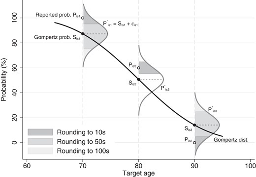
Illustration of the logic of the rounding model
The model is estimated using maximum simulated likelihood; Appendix F of the Supplementary Material presents the estimates. Observed covariates and individual and survey-wave effects generate a (prior) distribution for which captures variation in expectations. Average subjective expectations are calculated as the average 1-year survival probabilities across the distributions of observed and unobserved heterogeneity (based on 10,000 draws of individual and survey-wave effects). Hence, the subjective average is computed from the prior distribution of unobserved heterogeneity and does not condition on the probabilities or covariates reported by any given respondent.
Individual-specific expectations are approximated by the posterior mean of , conditional on the probabilities and observed covariates for a respondent. This modelling approach implies that expectations are exogenous, known at age 50, and vary over time only as a function of health. We focus on variation between rather than within individuals because respondents are observed for a relatively short period in the pre-reform sample (86% of respondents in the pre-reform period are observed in 1 or 2 waves). Moreover, fully exploiting longitudinal variation in subjective survival would add to the computational complexity of the model. Appendix F describes in detail how observed data, covariates and reported probabilities, are used to infer for each individual in the sample.
3 ESTIMATION
We apply a two-step procedure and estimate the processes for survival, health, medical expenses, wages, spousal income, and equivalence scales outside the retirement model. In step two, the preference parameters are estimated given those auxiliary processes by means of a Method of Simulated Moments (MSM) estimation algorithm (this is in line with much of the structural life cycle literature, e.g. French, 2005; De Nardi et al., 2010; French and Jones, 2011). For a given parameter vector, we simulate the life cycles of 5,000 workers using initial conditions taken from the data. Various target moments are calculated and compared to data by means of a Generalized Method of Moments objective function. The MSM estimator is the parameter vector that minimizes the difference between simulations and data moments. Finding this vector is complicated by the nature of the objective function, which is not uniformly differentiable and has multiple local minima. In light of such difficulties, we prefer simulated annealing over gradient-based optimization methods (we use the variant explained in Goffe et al., 1994). Appendix G of the Supplementary Material contains more details regarding the weighting matrix, objective function, and asymptotic distribution of the estimator.
The moments targeted in the second step concern labour supply, benefit claiming, and wealth. For labour supply, we match average yearly hours worked and participation rates by health status for 2-year age bins ranging from 50 to 65. Labour supply at ages 66–70 is not targeted, since the data show that workers with occupational pensions retire by age 65. These retirees no longer make labour supply decisions in the model. We match claiming rates for DI, UI, and occupational pensions by 2-year age brackets. Wealth is targeted through quartiles by age brackets: 2-year brackets for the ages 50–69 and 4-year brackets for ages 70–84 since there are fewer observations at the oldest ages. We match 91 moments in total (). Linear fixed effects models are used to remove cohort effects from the moments targeted in estimation, see Appendix H of the Supplementary Material for more information on the data moments.
All three versions of the model are estimated based on the same set of moments in order to level the playing field. No moments are targeted that condition on longevity, since life tables do not capture variation in expectations. Estimation of a model with heterogeneous survival expectations from moments that condition on survival is an interesting direction for future work.
While all parameters are affected by all moments in complex nonlinear models, we follow Eckstein et al. (2019) and provide a heuristic discussion of the identification of parameters in terms of the moments that are most important to pin them down. This is straightforward for the stigma costs of DI and UI, which are primarily determined by the corresponding claiming rates. Similarly, the leisure cost of poor health is driven by the difference in labour supply between poor and good health and the fixed cost of work by the combination of hours worked and the participation rate (higher fixed costs result in fewer hours of work at a given level of participation). It is more difficult to link the remaining parameters to specific groups of moments, since risk aversion, patience, the consumption weight, and the bequest motive all have profound effects on labour supply, benefit claiming, and wealth. We verified that the moments identify these parameters by fixing key parameters at different levels and estimating the rest. Comparing function values for these constrained estimation runs confirmed that the model cannot rationalize observed moments if we fix risk aversion, the discount factor, or the slope that relates household size to the importance of bequests at levels that are different from those obtained in unconstrained optimization. The parameter that allows the bequest weight to depend on the equivalence scale, the only new parameter in the specification of utility, is particularly sensitive to wealth holdings at ages older than 70. Fixing it at alternative values substantially worsens the fit of wealth profiles generated by the model.
4 DATA
We need rich data that cover a long period during the 1990s and 2000s in order to estimate the model and evaluate its predictions in a different policy regime. The DNB Household Survey (DHS, Centerdata, 1993–2016) is ideally suited to this purpose. The DHS is a yearly survey that is administered to the CentERpanel by CentERdata, which is affiliated with Tilburg University.18 The CentERpanel consists of roughly 5,000 individuals in 3,000 households and is representative for the Dutch population. Prospective members are selected at random from the address registry of Statistics Netherlands and are provided with internet access and a simple computer if required for participation. Panel members receive weekly questionnaires over the internet.
We model the labour supply and wealth of men who are at least 50 years old. Sample selection proceeds as follows. The auxiliary processes of (subjective) survival, health,19 medical expenses and equivalence scales are estimated on all 50+ men in the relevant DHS waves (1993–2001 for the estimation sample and 2006–16 for the out-of-sample predictions). Data moments to be targeted in estimation are computed from this sample after dropping men who were self-employed during any survey wave and those with fewer than 15 years of work experience (the self-employed are dropped because they are not covered by occupational pensions). Moreover, in order to isolate the groups with and without access to early retirement, we drop all men born after 1949 from the pre-reform sample. Similarly, we drop all men born before 1950 from the post-reform sample. We estimate the net income stream of the spouse on the partners of the men in these reduced samples.
Appendix H of the Supplementary Material describes the moments used to estimate preferences in detail. Appendix I of the Supplementary Material explains the sample selection and presents the first-step estimates for the auxiliary processes including survival. Appendix I of the Supplementary Material also contains descriptive statistics for the initial conditions.
5 ESTIMATION RESULTS
Table 2 presents preference estimates from the retirement model for the three sets of survival expectations. The leftmost column contains baseline results for the approach that relies on life tables. The estimated concavity parameter of the utility function is 4.64, which is in the ballpark established by previous literature. The consumption weight of 0.68, in line with the estimates around 0.60 reported in French (2005), indicates that consumption is valued more highly than leisure. At 1.04, the estimated discount factor implies a high degree of patience.20 Nonetheless, it is in line with previous work, in particular French (2005). Working any positive number of hours is associated with a fixed leisure cost of 1,085 hours/year (previous estimates are between 240 and 1,313 hours/year). The time cost of poor health is lower in the Netherlands at 131 hours/year compared with around 200 hours for the U.S. As a result, Dutch workers will reduce labour supply less strongly when they become unhealthy relative to their American peers. The estimated stigma costs indicate that disability and unemployment insurance come with sizable penalties of 1,681 and 3,620 hours of leisure, respectively, which strongly discourage claiming. As for bequests, the estimates suggest that they are directed primarily at other people living in the same household. The bequest weight of a man who lives with a partner is which declines to for a widower living alone. French (2005) estimates a constant bequest weight of 0.037, so bequests are much more important in the Netherlands. Individuals face less financial risk in the Dutch institutional context, which means the model needs a strong bequest motive to rationalize limited dissaving at advanced age. Moreover, the bequest curvature parameter is far from zero at 675,282 euro, which implies that the disutility of leaving zero bequests is finite.
Estimates for preference parameters
| (1) | (2) | (3) | |
|---|---|---|---|
| Life tables | Average subj. exp. | Heterogeneous exp. | |
| Utility functiona | |||
| σ (concavity) | 4.64 | 4.64 | 5.18 |
| (0.000023) | (0.000028) | (0.000038) | |
| κ (consumption weight) | 0.68 | 0.65 | 0.42 |
| (0.000061) | (0.000063) | (0.000065) | |
| β (discount factor) | 1.04 | 1.04 | 0.98 |
| (0.000026) | (0.000035) | (0.000028) | |
| ψ (fixed cost of work; hours/year) | 1085 | 1013 | 1101 |
| (27.5) | (4.5) | (8.0) | |
| (time cost of bad health; hours/year) | 131 | 249 | 251 |
| (13.9) | (34.6) | (6.9) | |
| ϕ (stigma cost DI; hours/year) | 1681 | 2029 | 2140 |
| (441.9) | (345.5) | (145.4) | |
| (stigma cost UI; hours/year) | 3620 | 3509 | 3568 |
| (8.9) | (1.9) | (5.9) | |
| Bequestsb | |||
| (intercept bequest weight) | 2.45 | 3.91 | -9.27 |
| (0.00014) | (0.00015) | (0.00010) | |
| (slope bequest weight) | 4.73 | 5.56 | 2.51 |
| (0.00012) | (0.00014) | (0.000082) | |
| K (concavity bequests) | 675,282 | 913,915 | 441,061 |
| (29.0) | (34.3) | (6.0) | |
| Function value | 473.27 | 473.21 | 483.89 |
Notes: Standard errors in parentheses. a; . b.
All standard errors in Table 2 are small relative to the point estimates. Such small standard errors are in line with previous work (e.g. Gustman and Steinmeier, 1986; Palumbo, 1999; Cagetti, 2003; French, 2005; French and Jones, 2011). One explanation is that the approximation of the GMM objective function as quadratic around the minimum may be poor for non-linear models (French, 2005). Furthermore, the reported errors do not reflect estimation uncertainty in the first-step estimates of the auxiliary processes. Finally, we target a wider variety of moments to fit the models than do other studies. Estimation uses moments that reflect wealth, labour supply, and benefit claiming whereas the literature mostly uses wealth and/or labour supply.
The middle column of Table 2 shows that the estimated concavity, consumption weight, and discount factor are similar when expectations are fixed at the average level in the subjective data. The estimated time costs of work, poor health, and UI benefit claiming change by many standard errors when we model survival expectations based on subjective data. Only for the cost of poor health is the change large relative to the estimate itself (it almost doubles from 131 to 249 hours). The most striking impact is on the estimates for the bequest motive. In particular, the dependence of the bequest weight on household size becomes stronger, which makes bequests relatively less important at older ages. Moreover, K increases from 675,282 to 913,915 euro, reducing the curvature in bequest utility. The net effect of these changes in expectations and parameters on model fit is negligible: the criterion values are almost identical at 473 for the specifications with expectations modelled by life tables and average subjective expectations without heterogeneity.
The final column of Table 2 introduces variation in mortality expectations, acknowledging that each individual has a unique view of his own longevity. Heterogeneity in expectations changes the estimates for most parameters substantially relative to estimation uncertainty. The most economically important changes relative to the model based on average subjective expectations are observed for the level of risk aversion, the consumption weight, the discount factor, and for the parameters associated with bequests. Agents modelled by the third set of estimates are more risk averse, care less about consumption, and are less patient than suggested by the other results. While these preferences are different in economically meaningful ways, all estimates remain plausible. The finding that subjective survival expectations increase risk aversion and decrease the discount factor relative to actuarial tables corroborates the results in Gan et al. (2015) in a richer life cycle model.
The bequest motive in model (3) is different from the other models in two ways. Firstly, the weight attached to bequests is much reduced, declining from 0.006 for a man living with his spouse to 0.001 for a widower. Secondly, the K parameter that governs the curvature of the bequest utility function drops from values above 600,000 euro for models (1) and (2) to 441,061 euro for the model with variation in beliefs. The implication is that the curvature of bequest utility is stronger than for the other two models: the marginal utility of leaving a bequest is higher at low levels and then drops as more wealth is bequeathed. These changes in preference parameters in combination with heterogeneous expectations result in a model fit that is similar to the other two models: the function value is 484. The next section shows exactly how the fit differs between the three models.
6 MODEL FIT
Figure 3 visualizes model fit by plotting data moments against their simulated counterparts based on all three specifications of expectations. Each column corresponds to a method used to approximate expectations and different rows show different groups of moments related to labour supply, benefit claiming, or wealth. Looking first at the baseline model based on life tables, panels (a) and (d) indicate that it succeeds to match observed labour supply reasonably well, especially for individuals in poor health. Labour supply in good health is overestimated by up to 200 hours/year or 10PP at ages 50–59. Some of this difference may be due to the assumption that there is no early retirement prior to age 59 while in reality some industries and employers did allow workers to retire earlier. When it comes to benefit claiming, the model fits claiming rates of occupational pensions and unemployment insurance closely, with the exception that it overestimates pension claiming at age 64–65 by 10PP. While it matches DI claiming well up to age bin 58–59, the model cannot rationalize the persistent claiming of disability insurance after early retirement becomes an option. The fit for wealth varies across the distribution. The first quartile of the simulated wealth distribution tracks the data closely at all ages. However, the median and third quartile fare worse, especially after age 74 when the model over-predicts net worth.
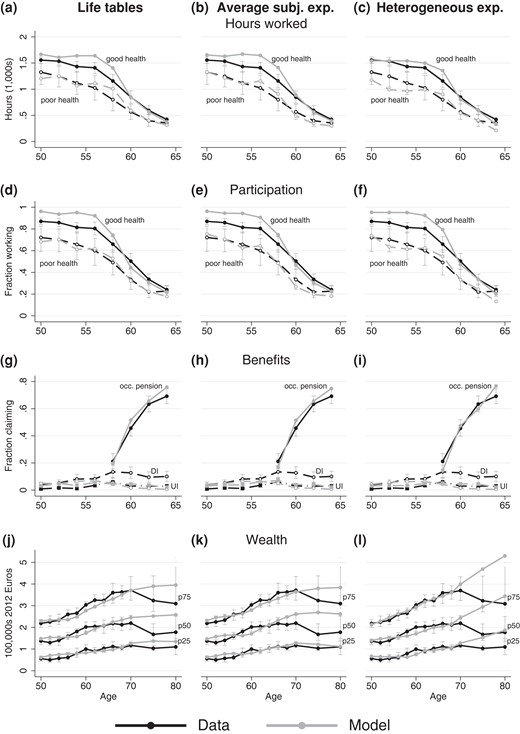
Model fit—target moments and simulations
The objective function values show that changing the level of survival probabilities to the average found in subjective data does not affect model fit. Figure 3 confirms that both models fit the data roughly equally well in all respects. Both models provide a better fit for labour supply in poor health than in good health. Panels (g) and (h) show that the models without variation in expectations are indistinguishable when it comes to claiming of pensions and benefits. Differences in terms of wealth are also small at all quartiles.
The model with heterogeneity in subjective expectations fits the data slightly worse than the other two models. This is the net result of a better fit for some moments and a worse fit for others. Panel (c) in the third column of Figure 3 shows that simulated hours worked in good health prior to age 60 are visibly closer to the data than for the other two models. While simulations stay within the 95% confidence intervals, the fit for labour supply in poor health deteriorates slightly. Panel (f) shows that the participation rate in good health is similar to the other models, but participation in poor health is not matched as well. Panel i. shows that there are no large changes in fit for pension claiming, or for disability and unemployment insurance. However, simulated wealth in panel (l) does look markedly different at ages 75–79 and 80–84. The simulated wealth quartiles for heterogeneous expectations continue to increase at those ages, while for the other two models wealth levels off. As a result, the third model fits the data less well in this respect. However, the deterioration in function value is small, 484 compared with 473, since wealth moments are estimated imprecisely at advanced age and the objective function places little weight on wealth at those age brackets. While there are statistically significant and economically meaningful differences between the estimated preferences, the fit of all three models shows similar strengths and weaknesses.
7 OUT-OF-SAMPLE PREDICTIONS
We use the models to predict changes in labour supply and pension claiming after a major pension reform. The most important change between the pre- and post-reform periods, 1993–2001 and 2006–16 respectively, was the introduction of actuarial adjustments to occupational pensions. Early claiming of occupational pensions was made less financially attractive for cohorts born in 1950 or later to encourage workers to delay retirement. Hence, the key outcome targeted by the policy reform was the age at which people first claim their pension: their retirement age. The top panel of Table 3 reports the average retirement ages in both policy regimes, as well as the difference between them. This is a before–after comparison in which the influence of cohort effects is mitigated by setting the pre-reform cohort to 1940–49 and the post-reform cohort to 1950–59 using linear fixed effects models as described in Appendix H of the Supplementary Material. The data indicate that the average retirement age increased from 61.2 to 63.8 when early retirement was made costlier. This increase of 2.6 years is consistent with quasi-experimental estimates of the effect of the abolishment of early retirement (e.g. Euwals et al., 2010). The recession following the 2008 financial crisis does not affect our estimate for the post-reform period substantially once we account for cohort differences between individuals born in the 1950s and 1960s.21
Average retirement age with (’93-’01) and without (’06-’16) generous early retirement schemes
| Pre-reform (1993–2001) | Post-reform (2006–16) | Difference (years) | |
|---|---|---|---|
| a. Data | |||
| Average pension agea,b | 61.2 | 63.8 | 2.6 |
| (60.97–61.41) | (63.49–64.03) | (2.23–2.92) | |
| N | 756 | 467 | 1223 |
| b. Simulations | |||
| Life tables | 60.7 | 65.9 | 5.2 |
| Average subj. exp. | 60.9 | 65.1 | 4.2 |
| Heterogeneous exp. | 61.0 | 63.7 | 2.7 |
Notes:aAge of retirement combines information from three sources: (1) actual retirement age reported by retirees; (2) observed retirement age if respondent retires while in the sample; (3) expected retirement age if neither reported nor observed retirement age is available. bRetirement ages below 50 or above 70 are set to missing; less than 1% of observations are dropped this way. 95% confidence intervals based on robust standard errors in parentheses.
The bottom panel of Table 3 shows that neither the model based on life tables nor that which fixes expectations at the level of average subjective beliefs successfully anticipates this observed change in behaviour. These models predict an average retirement age in the pre-reform sample of 60.7 and 60.9, respectively, only 4–6 months below the sample average of 61.2. However, both models substantially over-predict the retirement age for the period without early retirement with averages above age 65. These differences of 4–5 years relative to the pre-reform period are almost twice the 2.6 years observed in the data.
Allowing for individual-level variation in subjective mortality leads to similar in-sample retirement as the other models: on average people are predicted to retire at 61.0. However, that model produces much more reasonable simulations out-of-sample. In line with the data, it predicts that the average retirement age would increase to 63.7. The resulting difference between the two regimes is 2.7 years, close to the observed difference of 2.6 years.
Figure 4 provides more detailed information regarding observed and simulated labour supply under the two regimes. The figure shows the average hours worked by 2-year age bins (pooling individuals in good and poor health). Columns correspond to different models of survival expectations and the bottom graph in each panel highlights the difference between the pre- and post-reform periods. The solid lines in the top graphs reiterate the discussion of model fit within the estimation sample: all models fit the data similarly well and over-estimate labour supply prior to age 60, though the model with heterogeneous expectations does slightly better than the other two. The dashed lines correspond to the new policy regime and indicate that the models with homogeneous expectations, panels (a) and (b), substantially over-estimate labour supply out of sample for ages 60–63. While the data show that at those ages labour supply is 500 hours/year higher for the post-reform sample than before, these models produce differences of 900–1200 hours/year. Figure 4(c) confirms that out-of-sample simulations improve markedly once variation in life expectancy is taken into account. The differences in labour supply between data and simulations at ages 60–63 are less than half as large as those in panels (a) and (b). The bottom graph illustrates that the before–after comparison in the simulations from model 3 is much closer to the data. While all three models fit the data similarly well within-sample, variation in expectations generates substantially better out-of-sample forecasts.
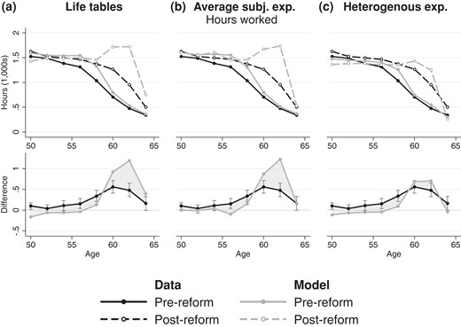
Simulated and observed labour supply in the pre-reform (1993–2001) and post-reform (2006–16) samples
The results in Figure 4 combine adjustments to the extensive and intensive margins. Appendix J of the Supplementary Material presents similar patterns for participation in the labour market. The appendix also presents a more extensive comparison of model predictions with post-reform data for all moments that are targeted in estimation. It corroborates that the model with heterogeneous survival expectations predicts claiming of occupational pensions after the reform much better than the other two models. Moreover, it shows that the better predictions for labour supply are driven by those in good health. Predicted labour supply in poor health at ages 60–63 is substantially higher than the data for all three models.
The simulations in Table 3 and Figure 4 provide a before–after comparison in which auxiliary processes (including survival), initial conditions, taxes, and pensions are all changed to the post-reform situation. While this provides a relevant basis for the external validation of the model, a policy maker running forecasts would not have access to post-reform data. Hence, we decompose the total effect from Table 3 into the contributions of initial conditions and auxiliary processes on the one hand and the tax and pension reforms on the other. Appendix K of the Supplementary Material provides the decomposition by changing one aspect at a time from pre- to post-reform. It shows that all three models attribute the change in retirement to the reform of occupational pensions. Both models with homogeneous expectations predict an excessively strong behavioural response, forecasting an average retirement age around 65 after the pension reform. Changing only the institutional rules for occupational pensions, the model with heterogeneous expectations continues to predict an average retirement age of 63.7, about 1 month younger than the average age in the data.
Since counterfactual predictions are better once individual-level heterogeneity in survival is taken into account, the question arises whether similar improvements can be had if one does not have access to subjective survival probabilities. Appendix L of the Supplementary Material explores limited heterogeneity across four groups defined by binary indicators for smoking and drinking. It combines actuarial tables with published estimates of the effects of these behaviours on survival. While the model with four groups predicts the same average retirement age before the pension reform as that with full heterogeneity, its counterfactual predictions are worse than any of the models discussed in the main text (the average simulated retirement age post reform is 67).
8 HOW DO HETEROGENEOUS EXPECTATIONS IMPROVE PREDICTIONS?
The previous section found that the model with variation in survival expectations generates more realistic counterfactual predictions than do models with homogeneous beliefs. This section shows how the interaction between preferences and expectations leads to better forecasts. We first analyse behaviour conditional on expectations in the pre-reform sample and then shift attention to the post-reform period.
8.1 Preferences, expectations, and behaviour before the reform
Figure 5 documents behaviour conditional on subjective survival. It presents moments by age bins separately for those who expect to live long (top 45% of subjective survival) or short (bottom 45%).22 Black lines correspond to data moments and grey lines represent model simulations. The data do not reveal large or statistically significant differences along survival expectations for hours worked, participation rates or pension claiming.23 However, small sample sizes result in wide confidence intervals for the differences between those who expect to live long and those who do not, so economically meaningful variation cannot be ruled out. Though these conditional moments were not targeted in estimation, the model with individual-specific expectations fits the data in that it does not generate large differences in labour supply or pension claiming.
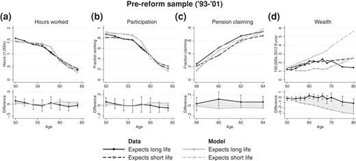
Behaviour conditional on survival expectations for the pre-reform sample (“long life” means top 45% of distribution of subjective survival, “short life” means bottom 45%)
The model does yield substantial covariation between wealth and life expectancy: those who expect to live shorter hold more wealth than their peers who expect a longer life. By age 80–84 the difference between the conditional medians amounts to 300,000 euro. This divergence is driven by the bequest motive, which is the primary driver of saving in the model. The Dutch institutional setting with automatic annuitization and generous social security limits the importance of precautionary and life-cycle considerations. Bequests are more important for those who expect a short life for two reasons. Firstly, they are expected to happen sooner and hence receive more weight in the decision process for those individuals who expect to die shortly. Secondly, the importance of bequests is a function of household size, which means they are relatively more important at younger ages. This motivates those with short life expectancy not only to accumulate more wealth but also to start that accumulation early. While uncertainty is considerable, the data do suggest that those who expect to live shorter hold on to more wealth after age 70. The point estimate for the difference at age 80–84 is 100,000 euro and the corresponding confidence interval does not include zero. However, up to age 70 there is little systematic covariation between wealth and expectations in the data, while in the simulations the difference quickly rises to 200,000 euro. While the model over-estimates differences in wealth holdings, it is broadly in line with the qualitative pattern observed at the oldest ages.
In order to understand why preference estimates change when expectations are made heterogeneous, Appendix M of the Supplementary Material compares simulations based on the model with heterogeneous expectations for two sets of preference parameters: the estimates obtained for average subjective expectations and those for heterogeneous subjective expectations. Simulated labour supply and benefit claiming are similar for both sets of preferences (see Figure M1 of the Supplementary Material). However, the model cannot rationalize positive wealth holdings after age 60 for at least one quarter of the sample at the preference estimates obtained for average subjective expectations. Figure M2 of the Supplementary Material indicates that this depletion of wealth reflects variation in expectations: median wealth for the top 45% of the distribution of subjective survival approaches zero by age 62. Furthermore, contrary to the data, the model produces larger differences in labour supply and pension claiming along the distribution of survival expectations. Comparing model simulations at these two sets of estimates illustrates how preferences and expectations interact. In particular, the fact that observed wealth does vary with survival but labour supply and pension claiming do not is valuable information regarding preferences.
8.2 Preferences, expectations, and behaviour after the reform
The pattern of unrealistically strong variation of behaviour with expectations when simulations are done at the preference estimates for average subjective survival is even starker in the post-reform sample (2006–16). Figure 6 displays differences in behaviour between those who expect to live long and those who anticipate an early demise. At the preference estimates for average subjective expectations, the variation in simulated labour supply and pension claiming across the distribution of expectations is more pronounced for this regime, in which occupational pensions are subject to actuarial adjustments. However, at the preference estimates for heterogeneous expectations both labour supply and pension claiming vary little with survival. Estimating preferences under heterogeneous expectations thus improves counterfactual predictions both overall and conditional on beliefs.
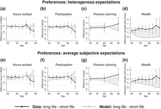
Differences in behaviour across the distribution of survival expectations for the post-reform sample (“long life” means top 45% of distribution of subjective survival, “short life” means bottom 45%)
Figure 7 illustrates which preference parameters are the most important drivers of differences in counterfactual predictions across models. The figure presents the average retirement age in simulations and the data for the period 2006–16. All simulations are based on the model with heterogeneous expectations but preferences vary. The leftmost bar corresponds to preference estimates for the same model and reproduces the average simulated retirement age of 63.7 (compared with 63.8 in the data, see Table 3). The rightmost bar is also based on the model with heterogeneous beliefs, but preferences are set to the estimates for the model that equates beliefs to the subjective average. Doing so results in an average simulated retirement age of 65.8, which is older than that based on the model with homogeneous expectations evaluated at the same parameters. The middle panel of Figure 7 illustrates the relative importance of the different parameters. It starts from the estimates obtained under belief heterogeneity and changes one parameter at a time to the estimate from the model without variation in expectations. Risk aversion (σ), the consumption weight (κ), the discount factor (β), and both parameters in the bequest weight ( and ) all have large effects on the average retirement age. These effects are intuitive: the intertemporal elasticity of substitution is higher in the model with homogeneous expectations, which makes agents less willing to work longer to increase consumption growth. This generates a smaller response in the retirement age when early retirement is made less attractive. The estimated consumption weight κ is also higher for homogeneous expectations, which makes agents value consumption over leisure and hence leads people to retire later. Raising the discount factor or making bequests more important have the same effect of delayed retirement. The estimates obtained for these parameters cause the model with heterogeneity to outperform the ones without it.
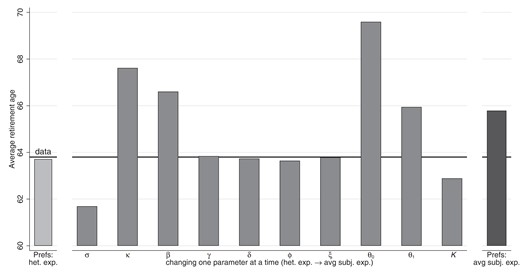
The impact of changing preference parameters on counterfactual simulations for the model with heterogeneous expectations
9 CONCLUSION
This article shows that individual-level variation in survival expectations derived from subjective probabilities improves the out-of-sample forecasts of a life cycle retirement model. We model the retirement incentives faced by Dutch workers during the 1990s, a period during which occupational pensions could be claimed as early as age 59 without actuarial adjustments to benefits. Preference parameters are estimated under three specifications for life expectancy: life tables adjusted for current health, average subjective expectations, and heterogeneous subjective expectations that use reported survival probabilities to construct subjective longevity for each individual in the sample. Using data from the DNB Household Survey for the period 1993–2016, we evaluate how survival expectations affect estimated preferences and model fit. The estimated preferences are then used to simulate behaviour in a policy regime that does adjust pension benefits for the age at which they are first claimed—the situation in place during the 2000s.
The findings show that expectations matter for the estimation of preferences: different models of expectations yield preference estimates that are both statistically and economically different. In particular, heterogeneity in expectations results in higher risk aversion, a lower weight on consumption relative to leisure, and a lower discount factor compared to the two models without variation in expectations. This extends the results in Gan et al. (2015) and underlines the idea that structural models identify preferences conditional on expectations (Manski, 2004).
While survival expectations affect preference estimates, the different combinations of expectations and preferences are largely equivalent in terms of implied behaviour prior to the pension reform. All three models match observed labour supply and occupational pension claiming, though they over-predict labour supply in good health for ages 50–59. They reproduce observed claiming rates for disability and unemployment insurance prior to the eligibility age for occupational pensions. They do not, however, match the sustained claiming of disability benefits once pensions become available. Moreover, while the models follow observed quartiles of wealth closely up to age bin 70–74, the median, and 75th percentile deviate from the data at older ages where those quartiles are estimated imprecisely. While the discrepancy in wealth is larger for the model with heterogeneous survival, the within-sample fit of all three models is similar overall.
We do find large differences in the accuracy of out-of-sample forecasts under alternative pension rules. The models based on life tables and average subjective expectations predict an average retirement age above 65 after the introduction of actuarial adjustments, an increase of 4–5 years relative to the estimation period. This increase is far larger than that observed in the DHS: the before–after difference in our sample is 2.6 years with an average post-reform retirement age of 63.8 years. The model with variation in survival expectations does much better, predicting a 2.7 year increase to an average of 63.7 (both are within the corresponding 95% confidence interval). The superiority of out-of-sample predictions from the model with heterogeneous beliefs is confirmed in more detailed analyses of labour supply by age. These improvements are not driven by covariation between labour supply or pension claiming and subjective longevity: neither in the data nor in simulations do we find systematic differences in behaviour between those with different life expectancies. Instead, the different preference estimates interact with expectations to produce more accurate forecasts. Risk aversion, the consumption weight, the discount factor, and the importance of bequests all play substantial roles. Changing these estimates affects labour supply, benefit claiming, and wealth accumulation, both overall and conditional on subjective longevity.
These findings illustrate the importance of heterogeneous expectations in structural economic models. Even though different combinations of expectations and preferences are roughly equivalent within a given institutional framework, they may still have very different implications in an alternative policy regime. Subjective probabilities elicited in surveys are a rich source of individual-level variation which models map into behaviour. This disciplines preferences without adding degrees of freedom, in contrast with latent preference types. It is plausible that heterogeneity in survival expectations matters for the counterfactual of actuarial adjustments to pension benefits, since those adjustments are designed to be fair only to someone with average mortality. The impact of other types of heterogeneity is a topic for future research. Examples include variation in choice intentions, e.g. retirement or bequest expectations, or variation in returns on investment.
Acknowledgments
This work is part of the research programme Innovational Research Incentives Scheme Veni with project number 451-15-018, which is financed by the Netherlands Organisation for Scientific Research (NWO). The code for the retirement model was adapted from that co-written with Pierre-Carl Michaud and Raquel Fonseca for De Bresser et al. (2017). I thank Pierre-Carl and Raquel for sharing their code and for the pleasant collaboration. The article benefitted substantially from the insightful comments of four anonymous referees and editor Áureo de Paula. I thank Max Groneck and David Sturrock for their careful discussions and Jeff Campbell and seminar participants at Berlin Applied Micro Seminar, Tilburg University, the 2018 Netspar Pension Day and the 2019 Netspar Pension Workshop for their feedback. Any remaining errors are my own.
Supplementary Data
Supplementary data are available at Review of Economic Studies online.
Data Availability Statement
The data and code underlying this research are available on Zenodo at https://dx.doi.org/10.5281/zenodo.8249573.
References
Footnotes
See De Nardi et al. (2016) for a review that is focused on saving and Blundell et al. (2016) for an overview of the literature on retirement.
Empirical work to date assumes that agents know the distribution from which future states are drawn: it allows for risk, but not for ambiguity. In a theoretical contribution, Groneck et al. (2016) show that ambiguity in survival expectations can explain under-saving at younger ages and slow decumulation of assets at advanced age, two stylized facts that characterize wealth profiles in the U.S.
Bach et al. (2020) and Fagereng et al. (2020) document persistent variation in returns to investment, which is another as yet unexplored margin of heterogeneity that could be relevant for life cycle models.
See Manski (2004) and Hurd (2009) for reviews of the literature on subjective expectations.
Subjective beliefs have been used in structural models of other decisions, where they mostly concern outcomes of decisions rather than exogenous processes such as mortality (Van der Klaauw, 2012; Pantano and Zheng, 2013). Examples include the perceived effectiveness of contraception (Delavande, 2008); the career perspectives of college majors (Zafar, 2011; Stinebrickner and Stinebrickner, 2013); and risk perceptions regarding HIV/AIDS and fertility (Shapira, 2017).
While the use of hold-out samples is most powerful if data remain embargoed during the model building phase (Schorfheide and Wolpin, 2012, 2016), this is not feasible for publicly available data such as the DHS.
The structural research that has employed validation through extrapolation has mostly relied on social experiments, in which one treatment arm is used for estimation and the others for validation. Examples include Wise (1985) on housing subsidies; Lise et al. (2004) on financial incentives to exit welfare; Todd and Wolpin (2006) on the PROGRESA experiment of cash transfers conditional on school attendance; Duflo et al. (2012) on financial incentives to reduce teacher absenteeism in India; Galiani et al. (2015) on location decisions in Boston; and Arcidiacono et al. (2021) on school vouchers in India.
In the data less than 1% of individuals report a retirement age outside the interval 50–70. We drop those observations from the validation exercise.
The equivalence scale at age t is the sample average across all households in which the male has age t: . The size of one such household may be larger than 2 if it contains (adult) children. This is the case for 38% of households in age bracket 50–60 and 7% for ages 61 and older.
The time endowment is based on hours per year that decision maker considers when deciding on work and leisure. That reserves a minimum of 7 hours per day for sleep and does not count weekends and 5 weeks of vacation. These constraints are assumed to be outside the individual’s control.
The overall curvature of bequest utility is governed by the risk aversion σ. K shifts around the “effective” level of bequests, which determines local curvature since the function is more curved at lower levels of bequests.
During the pre-reform period wealth tax was levied on the stock rather than on capital income.
The model limits the role of the spouse to the exogenous income stream and the equivalence scale to reduce computational complexity. An extended model that includes the spouse as an additional decision maker and explicitly accounts for her survival is left for future work.
Occupational pensions include a provision for the partner in case of widowhood. Modelling such partner pensions would require one to add the partner’s age and subjective longevity to the model as additional state variables. The model abstracts away from partner pensions to reduce computational complexity.
Linear random effects (RE) models of the reported probabilities that control for cubic polynomials in current age and target age show that the average reported probability of those in poor health is around 6–8PP lower than good health. Differences between education levels are small and not statistically significant, regardless of whether or not health is included in the model. Estimates are available on request.
Rounding is the tendency for respondents to report one number (e.g. 10%) when the true subjective probability lies in some interval (e.g. 5–15%). It has been shown to affect reported probabilities of many types (Manski and Molinari, 2010; De Bresser and Van Soest, 2013; Kleinjans and Van Soest, 2014; Bissonnette and de Bresser, 2018). The DHS induces additional rounding by eliciting expectations on a coarse 11-point response scale.
We divide both the target age and the current age by 100 to facilitate estimation of the baseline hazard α.
See https://www.centerdata.nl/en/databank/dhs-data-access for more information.
The binary measure for health is constructed by collapsing a five-point scale for subjective health into two categories. The bottom two levels, labelled “bad” and “not very good”, are combined into “bad” health, the top three into “good” health.
Because other studies sometimes fix the discount factor at a pre-determined value, we verified that our moments identify it by setting β to 0.97 and estimating the other parameters. Doing so yields a substantially worse objective function value.
Adding an indicator for the period after 2009, during which unemployment increased in the Netherlands, reduces the point estimate of the average retirement age during the post-reform period to 63.4 (95% confidence interval: 63.15–63.69). Hence, the difference between pre- and post-reform periods becomes 2.2 years (confidence interval: 1.89–2.57).
The top 45% of subjective survival corresponds to the bottom 45% of posterior means for individual effects for the hazard of death and vice versa. We drop the middle 10% of the sample to make the classification more robust to measurement error in the reported probabilities used to model beliefs. Grouping based on individual effects from linear models as explained in Appendix F of the Supplementary Material results in very similar high and low survival groups (92% of respondents are allocated to the same group).
The absence of substantial variation in labour supply and pension claiming across the distribution of subjective longevity is not an artefact of data processing such as the removal of cohort effects, since it is confirmed for raw claiming and labour supply (estimates available on request).
Author notes
The editor in charge of this paper was Aureo de Paula.
