A Theory of Monetary Union and Financial Integration

Abstract

Since the creation of the euro, capital flows among member countries have been large and volatile. Motivated by this fact, I provide a theory connecting the exchange rate regime to financial integration. The key feature of the model is that monetary policy affects the value of collateral that creditors seize upon default. Under flexible exchange rates, national governments can expropriate foreign creditors by depreciating the exchange rate, which induces investors to impose tight constraints on international borrowing. Creating a monetary union, by eliminating this source of currency risk, increases financial integration among member countries. This process, however, does not necessarily lead to higher welfare. The reason is that a high degree of capital mobility can generate multiple equilibria, with bad equilibria characterized by inefficient capital flights. Capital controls or fiscal transfers can eliminate bad equilibria, but their implementation requires international cooperation.

1. Introduction

What are the benefits and costs from adopting a common currency? This question has been at the centre of a long-standing debate in international macroeconomics. In a seminal paper, Friedman (1953) claimed that flexible exchange rates act as shock absorbers, so that fixing exchange rates will generate welfare losses by increasing macroeconomic volatility. Instead, while writing about the European monetary integration, Ingram (1973) provided a more positive view of currency unions. He argued that forming a currency union will foster financial integration among member countries, leading to a more efficient international allocation of capital and higher welfare.

Ingram’s view resonates well with some aspects of the euro area experience. Indeed, the introduction of the euro has been accompanied by a sharp increase in financial flows among member countries (Lane, 2006). Moreover, existing empirical evidence suggests that the elimination of currency risk has been the main driver behind the euro’s positive impact on financial integration (Kalemli-Ozcan et al., 2010). But some crucial questions are open. First, why should the exchange rate regime matter for financial integration and capital flows? And does higher capital mobility necessarily lead to higher welfare, especially in light of the fact that several euro area countries suffered crisis periods characterized by financial instability and capital flights?¹

In this article, I tackle these questions by providing a theory connecting the exchange rate regime to international financial integration. There are three frictions at the heart of the model. The first one is the presence of nominal wage rigidities, a classic friction in monetary economics, which implies that monetary policy has real effects on output. The second friction, typical of the macro-finance literature, is that output is used as collateral to perform financial transactions. As we will see, the combination of these two frictions creates a link between monetary—and exchange rate—policy and financial flows. The third friction is that monetary authorities lack the ability to commit.

The first result of the article is that, in accordance with Ingram’s view, forming a currency union increases financial integration among member countries. The reason is simple. In the model, an exchange rate depreciation reduces the value of the collateral that foreign investors repossess when domestic agents default. National governments thus face a time-consistency problem. Once the external debt of a country exceeds a threshold, it is optimal for the government to engineer a depreciation to expropriate foreign creditors. To escape expropriation, international investors respond by imposing ex ante tight constraints on international borrowing. Under flexible exchange rates, therefore, international capital mobility is limited.

It is often claimed that investors can escape currency risk by denominating debt contracts in a foreign currency or in real terms. This is not the case here, since expropriation occurs because the exchange rate affects the value of collateral backing financial contracts. This feature sets the model apart from the literature on nominal debt and limited commitment over monetary policy (Bohn, 1990), in which the central bank’s time-consistency problem can be solved by issuing debt contracts denominated in a foreign currency or in real terms. In contrast, addressing the time-consistency problem studied by this article requires more fundamental changes in the monetary framework, such as forming a currency union.²

In a monetary union national governments delegate monetary policy to a supranational authority, the union’s central bank, which acts in the interest of all member countries. Unlike national governments, the union’s central bank does not have a strong incentive to expropriate creditors, as long as they belong to the union. Joining a currency union thus imposes a vincolo esterno—that is an external constraint—on national governments, preventing them from using monetary policy to expropriate foreign creditors.³ Hence, in a currency union countries can sustain a higher stock of foreign debt toward other members without defaulting. Adopting a common currency thus increases international capital mobility within the monetary union.⁴

Does this process lead to efficient capital flows and higher welfare? I first show that forming a monetary union might increase welfare by fostering capital flows toward countries in which capital is most productive. For this to happen, two conditions have to be met. First, there must be some asymmetry in terms of investment opportunities among member countries. This result contrasts with the traditional optimal currency area literature, in which giving up exchange rate flexibility is costly precisely when countries are asymmetric (Mundell, 1961). Second, financial frictions need to be severe enough to prevent an efficient international allocation of capital under flexible exchange rates. Hence, adopting a common currency is optimal only if financial markets are not too developed to start with.

But this benign view does not square well with the recent experience of the euro area, characterized by financial instability and volatile capital flows. As argued by a vast literature, financial instability might be the result of complementarities in investment decisions (Akerlof, 2019). Building on this insight, I introduce investment complementarities by considering an economy in which governments finance some fixed expenditure with taxes on capital income. This opens the door to fluctuations in capital flows purely driven by animal spirits.⁵ Expectations of high taxes on capital, the logic is, can trigger a capital flight and a fall in domestic investment. The associated fall in the tax base forces the government to raise taxes, inducing another round of capital flights. This feedback loop can make pessimistic expectations self-fulfilling and give rise to capital flights out of high-productivity countries.

Importantly, episodes of inefficient capital flights can take place only if financial integration is sufficiently high. Therefore monetary unions, with their inherent high degree of capital mobility, are particularly prone to experience expectations-driven fluctuations in capital flows.⁶ Forming a monetary union might thus lower welfare, by inducing volatility in international financial flows and capital misallocation. Furthermore, inefficient capital flights are more likely to happen when a monetary union is hit by large shocks requiring a fiscal response, such as large financial crises or pandemics. In this respect, the model suggests that participating in a common currency might hamper national governments’ ability to react to shocks through fiscal policy, due to high capital mobility and the risk of capital flights driven by pessimistic animal spirits.

A natural question to ask is what policy interventions can prevent self-fulfilling capital flights from taking place. One possibility is to impose controls on capital flows. Another option is to set up a system of countercyclical fiscal transfers among the countries of the union, in the spirit of Kenen (1969) and Farhi et al. (2014). If credible, the presence of a countercyclical transfers scheme anchors agents’ expectations on the good equilibrium, in which capital flows toward high-productivity countries. Volatility in capital flows driven by animal spirits is thus ruled out, without the need to actually transfer resources among countries in equilibrium.

While these policies are beneficial from a global perspective, however, they might lower welfare for some countries in the union. In fact, during episodes of inefficient capital flights some member countries act as safe havens, and so benefit from inflows of cheap foreign capital. Implementing policies that rule out capital flights driven by pessimistic expectations might then lower welfare in safe-haven countries. Successfully managing financial integration in a monetary union is therefore possible, but requires close international cooperation.

Related literature. This article contributes to the optimal currency area literature, which studies the costs and benefits associated with forming a monetary union. Friedman (1953) argues that joining a monetary union is costly, because the loss of independent monetary policy leads to higher output volatility in response to asymmetric shocks. Benigno (2004) and Fornaro (2018) provide modern formulations of this argument using New Keynesian open-economy models. A large literature has considered factors that mitigate the impact on welfare of asymmetric shocks in monetary unions. To cite a few examples, Mundell (1961) and Farhi and Werning (2014) stress the role of labour mobility, Kenen (1969), Gali and Monacelli (2008), and Farhi et al. (2014) focus on fiscal transfers, Farhi and Werning (2017) consider fiscal devaluations, Farhi et al. (2014), Schmitt-Grohé and Uribe (2016), and Sergeyev (2016) study macroprudential policies, while Aguiar et al. (2015) and Bianchi and Mondragon (2021) focus on public debt and rollover crises. A smaller body of work has studied the benefits derived from creating a monetary union. For instance, in Giavazzi and Pagano (1988) and Alesina and Barro (2002) countries might wish to join a currency union in order to reduce inflation. In Rey (2001) and Alesina and Barro (2002), sharing a common currency reduces the cost of performing international transactions and facilitates trade. Nurkse (1944), Jeanne and Rose (2002), and Gabaix and Maggiori (2015) argue that flexible exchange rates, rather than acting as shock absorbers, can be a source of volatility by triggering speculative flows. None of these papers study the impact of the exchange rate regime on financial integration.

The notion that creating a monetary union will lead to higher financial integration has a long history (Keynes, 1930; Ingram, 1973), and was very much present in the debate paving the way to the euro adoption (Giavazzi, 1989), but few attempts have been made at formalizing this insight. To the best of my knowledge, in fact, Doepke and Schneider (2017) provide the only other framework in which forming a monetary union increases financial integration among member countries. The key friction in Doepke and Schneider (2017) is that financial contracts are non-contingent and defaulting generates social losses. Sharing a common currency leads to higher international financial integration because it limits the probability that agents default in response to exogenous shocks. The channel emphasized by this article is very different. In fact, my argument does not rest on the inability to write contingent contracts, but rather on the combination of nominal wage rigidities and collateral constraints. Moreover, in Doepke and Schneider (2017) monetary policy is exogenous, while in this article the endogenous response of monetary policy to capital flows plays a crucial role.⁷ Finally, in Doepke and Schneider (2017) increasing financial integration is welfare improving. Here, instead, higher financial integration may generate financial instability and welfare losses.

A small literature has studied the interplay between the exchange rate regime and access to foreign credit in small open economies settings. In Arellano and Heathcote (2010) governments finance their expenditure through seignorage or foreign borrowing, and they are punished with exclusion from credit markets in case of default. Fixing the exchange rate—and so giving up seignorage—exacerbates the cost of being excluded from the credit markets and thus increases the government’s debt limit. Closer to this article, Fornaro (2015), Ottonello (2021), and Coulibaly (2018) study economies in which monetary policy affects collateral value because of the presence of nominal wage rigidities. These works, however, abstract from the time-consistency problem which is at the heart of this article, by assuming that national governments can commit not to use monetary policy to expropriate foreign investors. Furthermore, in Fornaro (2015), Ottonello (2021), and Coulibaly (2018) fixing the exchange rate triggers a process of reduction in foreign debt, which seems inconsistent with the experience of peripheral countries during the first ten years of the euro. Another important difference is that all these works focus on single small open economies, while this article studies a multi-country economy, in which global credit markets clear. This allows me to model how the exchange rate regime affects the potential for capital outflows by domestic agents, a dimension which is absent in Arellano and Heathcote (2010), Fornaro (2015), Ottonello (2021), and Coulibaly (2018). This aspect is crucial to understand why currency unions might be particularly exposed to capital flows volatility and episodes of inefficient capital flights.

The paper is also related to Tirole (2003) and Jeanne (2009), who study settings in which placing constraints on government policy facilitates international borrowing, because it limits the government’s ability to expropriate foreign investors. Compared to these papers, I focus on an alternative channel through which expropriation can occur, given by the interplay between monetary policy and collateral value. Moreover, both Tirole (2003) and Jeanne (2009) consider a single country. Instead, a key element of this article is its multi-country dimension, and in particular the fact that forming a currency union facilitates financial flows both in and out of member countries. Because of this reason, the impact of higher financial integration on welfare is ambiguous in my model, while it is positive in Tirole (2003) and Jeanne (2009).

Finally, this article is connected to the literature emphasizing how increasing international financial integration can have an ambiguous impact on welfare. Two examples are Martin and Rey (2006) and Broner and Ventura (2016). In both papers, a high degree of financial integration may open the door to pessimistic equilibria characterized by inefficient capital flights. However, these papers take the level of international financial integration as determined by exogenous forces. Here financial integration is endogenously determined, and depends on the exchange rate regime.

The rest of the article is composed of five sections. Section 2 presents the baseline model. Section 3 describes the connection between the exchange rate regime and financial integration. Section 4 derives the implications for capital flows and welfare. Section 5 discusses some policy implications for monetary unions. Section 6 concludes. The Appendix contains all the proofs and derivations not included in the main text.

2. Model

Consider a world composed of two countries, home and foreign. There are two periods: 0 and 1. In period 0 agents sign financial contracts and make their investment decisions. In period 1 production takes place, financial contracts are settled and agents consume. Agents are rational and there is perfect foresight.

To simplify the exposition, while presenting the model I will focus on the home economy. The foreign country is, however, characterized by exactly the same equilibrium conditions. When needed, I will denote variables pertaining to the foreign country with |$*$| superscripts.

2.1. Households

The home country is populated by a continuum of measure one of identical households. Households consume and work in period 1 only, and their utility is

$$ \begin{equation*} C_T + \frac{C_N^{1-\eta}}{1-\eta} - L.\end{equation*}$$

In this expression, |$C_T$| and |$C_N$| denote respectively consumption of a tradable and a non-tradable good, while |$L$| denotes labour effort.⁸

In period 0 households are endowed with |$N$| units of the tradable good. There are two assets in which households can invest to transfer tradable goods to period 1. First, households can invest in a domestic technology, call it capital, that transforms one unit of the tradable good in period 0 into |$A$| units of the tradable good in period 1. Let |$I$| denote investment in home-country capital. In addition, households have access to a real bond denominated in units of the tradable good. Denote by |$D$| the level of debt assumed by domestic households in period 0 and due in period 1, and |$R$| the gross interest rate between the two periods. The bond is traded internationally, and |$R$| is common across the two countries.

The period 0 budget constraint of home households is thus given by

$$ \begin{equation}\label{BC} I = N + \frac{D}{R}.\end{equation}$$

(1)

Moreover, as it will become clear later on, each household faces a borrowing limit

$$ \begin{equation*} D \leq \bar{D}. \end{equation*}$$

Households’ optimal investment strategy is then

$$ \begin{equation}\label{II} I = \begin{cases} N + \frac{\bar{D}}{R} & \quad \text{if } A > R\\ \left[0, N + \frac{\bar{D}}{R}\right] & \quad \text{if } A = R \\ 0 & \quad \text{if } A < R. \end{cases} \end{equation}$$

(2)

Intuitively, if |$A>R$| households maximize investment in domestic capital by borrowing up to their limit. Instead, if |$A<R$| investment in domestic capital is unprofitable, and households lend all their net worth on the international credit markets. Finally, if |$A=R$| households are indifferent between investing in domestic capital and lending on the credit markets.

In period 1, households receive the return from period 0 investment, work, and consume. Their period 1 budget constraint in terms of the home currency is

$$ \begin{equation*} P_T C_T + P_N C_N = P_T Y_T - P_T \mathcal{R} + W L. \end{equation*}$$

The left-hand side of this expression represents the households’ expenditure. |$P_T$| and |$P_N$| denote respectively the price of a unit of tradable and non-tradable good in terms of the home currency. Hence, |$P_T C_T + P_N C_N$| is the total nominal expenditure in consumption. Since period 1 is the terminal date of the economy, households hold no assets at the end of the period.

The right-hand side captures the households’ income. |$Y_T$| denotes the output of tradable goods produced by the home country in period 1, given by

$$ \begin{equation}\label{YT} Y_T = AI. \end{equation}$$

(3)

|$\mathcal{R}$| is the amount of loan repayment that households make in period 1. |$W$| denotes the nominal wage, and hence |$W L$| is the households’ labour income.

In period 1, households have two decisions to make. First, each household chooses whether to honour its debt or default. In case of default, creditors appropriate a fraction |$\kappa$| of the household’s income, so that the household is left with the complement fraction |$1-\kappa$|⁠. Households thus default if their debt exceeds the value of the collateral that creditors repossess upon default. This implies that

$$ \begin{equation*} \mathcal{R} = \min \left[ D, \kappa \left(Y_T + \frac{W}{P_T} L\right) \right]\!. \end{equation*}$$

In words, the payment that households make to their creditors cannot exceed a fraction |$\kappa$| of their income. The assumption that defaulting triggers a fall in the borrower’s income follows a vast literature in macroeconomics. It is, indeed, commonly made in the sovereign default literature (Eaton and Gersovitz, 1981). It is also close in spirit to the friction considered by Kiyotaki and Moore (1997), but with the household’s income instead of capital as collateral.⁹

Second, households allocate expenditure between the two consumption goods. This leads to the demand function for non-tradable goods

$$ \begin{equation}\label{CNd} C_N = \left( \frac{P_N}{P_T}\right)^{-\frac{1}{\eta}}. \end{equation}$$

(4)

Demand for non-tradables is thus decreasing in their relative price |$P_N/P_T$|⁠.

2.2. Nominal wage rigidities

To allow for real effects from monetary policy, I introduce a simple friction in the adjustment of nominal wages. In particular, nominal wages are fixed and equal to |$W$|⁠. To clear the labour market, I then assume that households satisfy firms’ labour demand.

To be clear, the results that follow do not rely at all on this extreme form of wage rigidity, and would extend to a setting in which partial adjustment of nominal wages is possible. But considering an economy with fixed wages is convenient, because it simplifies the analysis and allows for a transparent characterization of the economic forces at the heart of the model.

2.3. Non-tradable production and the real exchange rate

Non-traded output |$Y_N$| is produced by a large number of competitive firms. Labour is the only factor of production, and the production function is |$Y_N = L$|⁠. Profits are given by |$P_N Y_N - W L$|⁠. The zero profit condition implies that in equilibrium |$P_N = W$|⁠.

Throughout the article, I will define the real exchange rate of a country as the price of its non-tradable good relative to the tradable one. The real exchange rate of the home economy, denoted by |$p$|⁠, is then given by

$$ \begin{equation}\label{RER} p =\frac{P_N}{P_T} = \frac{W}{P_T}. \end{equation}$$

(5)

Notice that, since the nominal wage is rigid, changes in the nominal price of the tradable good affect the real exchange rate. In fact, as I will explain later on, this is the channel through which monetary policy affects the real economy.

2.4. Market clearing and equilibrium

Market clearing for the non-tradable consumption good requires that domestic consumption is equal to domestic production

$$ \begin{equation}\label{CN} Y_N = C_N. \end{equation}$$

(6)

Combining this condition with equation (4) gives

$$ \begin{equation}\label{AD} Y_N = p^{-\frac{1}{\eta}}. \end{equation}$$

(7)

Hence the real exchange rate, through its impact on demand, effectively determines production of non-tradable goods.

In equilibrium, tradable consumption must be equal to tradable output less the payment made to foreign creditors. Using the fact that households’ income is equal to aggregate output, the market clearing condition for tradable goods can be written as

$$ \begin{equation}\label{COL} C_T = Y_T -\min\left[D, \kappa \left(Y_T + p Y_N\right)\right]\!. \end{equation}$$

(8)

As highlighted by this equation, collateral is thus equal to a fraction |$\kappa$| of the value of the country’s output in terms of the tradable good. This happens because foreign creditors cannot consume non-traded goods produced by the home country. Hence, when foreigners repossess non-tradable goods from defaulting debtors they need to sell them at price |$p$| in exchange for tradable goods.

Combining (7) and (8) gives an expression linking the value of collateral to the real exchange rate

$$ \begin{equation*} \kappa \left(Y_T + p^{1-\frac{1}{\eta}}\right)\!. \end{equation*}$$

In principle, the relationship between the real exchange rate and collateral value is ambiguous and depends on |$\eta$|⁠. The results that follow only require that movements in the real exchange rate affect collateral value, and so that |$\eta \neq 1$|⁠. But, purely to simplify the exposition, from now on I will assume that |$\eta > 1$|⁠.¹⁰ In this case, a real exchange rate depreciation reduces the value of collateral. Analogous market clearing conditions hold for the foreign economy.

Finally, the global market clearing conditions are

$$ \begin{align}\label{GMK1} N + N^* = I + I^*\\ \end{align}$$

(9)

$$ \begin{align}C_T + C_T^* = Y_T + Y^*_T.\label{GMK2} \end{align}$$

(10)

Equation (9) ensures that global investment in capital is equal to the world endowment of the tradable good in period 0. Equation (10) implies that period 1 global consumption of tradable goods is equal to global production.

We are now ready to define a competitive equilibrium.

Definition 1.

A competitive equilibrium is a set of real allocations ⁠, and world interest rate |$R$|⁠, satisfying (1), (2), (3), (6), (7), (8)—plus their counterparts for the foreign country—and (10), given policy-determined values for the real exchange rates |$\{p, p^*\}$| and for the debt limits |$\{\bar{D}, \bar{D}^*\}$|⁠.

2.5. Discussion of assumptions

The key feature of the model is that monetary policy can influence the payment that foreign creditors receive from domestic agents. This happens because monetary policy affects the real exchange rate, and so the value in terms of tradables of the domestic production of non-traded goods. However, several other assumptions would give rise to similar results. For instance, in the spirit of Kiyotaki and Moore (1997), one could consider a setting in which collateral is given by some long-lived asset, such as capital, land, or housing. As long as monetary policy has an impact on the foreign currency value of this asset, as for instance in Fornaro (2015), the main results of the article go through.

Another possibility is to consider debt contracts denominated in domestic currency. Also in this case, in fact, monetary policy would affect the payment received by foreign creditors. However, as documented empirically by Maggiori et al. (2020), foreign creditors rarely accept to sign debt contracts denominated in domestic currency. This is the reason why the model considers debt contracts denominated in real terms, which cannot be directly affected by monetary policy. In fact, one could even assume that agents sign equity—rather than debt—contracts. As long as their payment is backed up by collateral, all the main results would still apply.

Finally, let me clarify that all the results that follow would go through if one were to assume that |$\eta < 1$|⁠. The only difference is that in this case monetary authorities would need to appreciate the exchange rate in order to expropriate foreign investors. The same consideration applies to the model studied by Fornaro (2015), in which exchange rate depreciations increase land price and collateral value. In this case, the expropriation of foreign investors would take place through an appreciation of the exchange rate, leading to a drop in land price and collateral value.

3. Exchange Rate Regime and Financial Integration

What is the relationship between monetary policy, the exchange rate regime and financial integration? To answer this question, I solve the model backward and start by characterizing the equilibrium in period 1. Throughout I will contrast two different policy regimes. First, I will consider the case of flexible exchange rates. I will then turn to the case of a monetary union.

3.1. Flexible exchange rates

In this simple model monetary policy amounts to setting a value for the nominal price of the tradable good.¹¹ Under flexible exchange rates each country can run its own independent monetary policy. To see this point, start by considering that the law of one price for the tradable good implies

$$ \begin{equation*} P_T = S P_{T}^{*}, \end{equation*}$$

where |$S$| denotes the nominal exchange rate, defined as the units of home currency needed to purchase one unit of the foreign currency. The key observation is that the nominal price of the traded good can differ across the two countries, because the nominal exchange rate adjusts to make sure that the law of one price holds. Thus, under flexible exchange rates national governments can freely control the domestic nominal price of the traded good. Since nominal wages are rigid, the implication is that national governments can set their real exchange rate.

Closing the model requires specifying how monetary policy is conducted. I consider governments that implement the optimal non-cooperative monetary policy. Therefore, each government seeks to maximize the welfare of its country’s citizens, without any concern for welfare in the rest of the world. Moreover, each government operates under discretion. This means that governments set monetary policy in period 1, without being restricted by any promise that they might have made in period 0.

For instance, in period 1 the home government chooses |$p$|⁠, |$Y_N$|⁠, and |$C_T$| to maximize home households’ utility

$$ \begin{equation*} C_T + \frac{Y_N^{1-\eta}}{1-\eta} - Y_N, \end{equation*}$$

where I have used the equilibrium conditions |$C_N = Y_N = L$|⁠. Utility is maximized subject to

$$ \begin{gather*} Y_N = p^{-\frac{1}{\eta}}\\ C_T = Y_T - \min \left[ D, \kappa \left(Y_T + p^{1-\frac{1}{\eta}}\right) \right]\!. \end{gather*}$$

Hence, by setting |$p$| the government affects two margins. First, |$p$| determines the quantity of non-tradable goods produced and consumed by domestic households. Second, if the home country is in a default state, the real exchange rate affects the value of the collateral that foreign creditors repossess from domestic agents.

I will characterize the government policy in two steps.¹² The first step consists in deriving the optimal value for the real exchange rate, conditional on whether the country is in a default state or not. Start by assuming that |$D <\kappa \left(Y_T + p^{1-\frac{1}{\eta}}\right)$|⁠, so that home agents do not default. Then, it is optimal for the home government to set

$$ \begin{equation*} p = 1 \rightarrow Y_N = 1. \end{equation*}$$

To understand this condition, consider that |$Y_N = 1$| is the natural level of non-tradable output, that is the amount of non-tradable goods that the economy would produce in absence of nominal rigidities.¹³ Hence, conditional on no default, the optimal monetary policy offsets the impact of nominal rigidities on production.

Now imagine that |$D > \kappa \left(Y_T + p^{1-\frac{1}{\eta}}\right)$|⁠, so that home households are defaulting on their creditors. In this case, the home government sets

$$ \begin{equation*} p = \left(1+\kappa (\eta-1)\right)^{-1} < 1 \rightarrow Y_N > 1. \end{equation*}$$

In case of default the government has thus an additional incentive to depreciate the exchange rate. An exchange rate depreciation, in fact, reduces the value of collateral and thus the amount of tradable goods that foreign creditors can extract from domestic households. The counterpart of this exchange rate depreciation is the overheating of the domestic economy, in the sense that output of non-tradable goods ends up being above its natural level (⁠|$Y_N > 1$|⁠). So, conditional on defaulting, the home government trades off the gains from depreciating the exchange rate to expropriate foreign creditors, with the costs associated with an inefficiently high production of the non-tradable good.

The second step consists in deriving the conditions under which default occurs. Naturally, the country defaults whenever doing so delivers higher welfare compared to repaying. After some algebra, one finds that default occurs if

$$ \begin{equation*} D > \kappa Y_T + \frac{\eta}{\eta-1} \left[ \left( 1+ \kappa (\eta-1)\right)^{\frac{1}{\eta}}-1 \right] \equiv \bar{D}_\textit{flex}. \end{equation*}$$

In words, the home country defaults whenever its foreign debt is higher than the threshold |$\bar{D}_{flex}$|⁠. The following proposition summarizes these results.¹⁴

Proposition 1.

Under flexible exchange rates, the home country does not default if and only if |$D \leq \bar{D}_\textit{flex}$|⁠. Moreover, in absence of default monetary policy sets |$p = Y_N = 1$|⁠. Analogous expressions hold for the foreign country.

A couple of remarks are in order. First, since agents are rational, ex-ante investors will never lend to the home country more than |$\bar{D}_\textit{flex}/R$|⁠. Otherwise, the home country would default and creditors would make a loss. It follows that the debt ceiling imposed by foreign investors under flexible exchange rates is |$\bar{D} = \bar{D}_\textit{flex}$|⁠.¹⁵ This also means that countries never accumulate enough debt to trigger a default, and so in equilibrium monetary policy sets |$p = Y_N = 1$| to replicate the allocation under flexible wages.

Second, under flexible exchange rates the debt ceiling imposed by foreign investors is lower than the value of collateral observed in equilibrium. In fact, it is easy to check that

$$ \begin{equation*} \bar{D}_\textit{flex} < \kappa \left(Y_T + p Y_N\right) = \kappa \left(Y_T + 1\right)\!. \end{equation*}$$

This happens because foreign investors anticipate that, if they were to lend to the home country slightly more than |$\bar{D}_\textit{flex}$|⁠, the government would engineer a discrete depreciation of the real exchange rate. In turn, the depreciation would trigger a discrete fall in the value of collateral. Hence, under flexible exchange rates, a naive observer would conclude that borrowers never borrow enough to exhaust the value of their collateral.¹⁶

To end this section, notice that national governments are subject to a time-consistency problem. In period 0, in fact, the government would like to commit not to depreciate the exchange rate in period 1. This would relax the borrowing limit imposed by investors on domestic agents. However, when period 1 comes the government has an incentive to forget its past promises and to expropriate foreign creditors through a depreciation. In absence of commitment, the period 0 promise not to devalue the exchange rate ex post is thus not credible. This commitment problem is precisely the reason why the debt ceiling imposed by foreign investors is lower than the amount of collateral observed in equilibrium.¹⁷

Interestingly, this time-consistency problem is present even though debt is denominated in real terms, rather than in terms of the domestic currency. This feature sets the model apart from the literature on nominal debt and limited commitment over monetary policy (Bohn, 1990; Araujo et al., 2013; Engel and Park, 2018; Ottonello and Perez, 2019), in which the central bank’s time-consistency problem can be avoided by signing debt contracts in real terms or in terms of a foreign currency. The limited commitment problem at the heart of this model, instead, cannot be solved by changing the currency denomination of debt, or even by signing equity—rather than debt—contracts. As we will see, addressing it requires more fundamental changes in the monetary framework, such as forming a currency union.

3.2. Monetary union

I now turn to the case of a monetary union.¹⁸ In a monetary union, the two countries share the same currency and so |$S=1$|⁠. The law of one price for the tradable good then implies that |$P_T = P^*_T$|⁠, so that differences in the nominal price of tradables across countries cannot arise.

Moreover, monetary policy is no longer controlled by national governments. It is instead set by a supranational authority, the union’s central bank. To parallel the case of flexible exchange rates, I consider a benevolent central bank that operates under discretion. The key difference is that the central bank of the union seeks to maximize the welfare of the union as a whole. More concretely, I assume that the central bank attaches equal weight to the welfare of every citizen of the union.

In principle, the home and foreign country could have different pre-set nominal wages. To keep the analysis transparent, it is however convenient to assume that |$W = W^*$|⁠. Under this condition, both countries feature the same real exchange rate and the same production of non-traded goods (⁠|$p = p^*$|⁠, |$Y_N = Y_N^*$|⁠).

The union’s central bank thus maximizes

$$ \begin{equation*} Y_T + Y_T^* + 2 \left(\frac{Y_N^{1-\eta}}{1-\eta} - Y_N\right)\!, \end{equation*}$$

where I have used the market clearing condition |$C_T + C_T^* = Y_T + Y_T^*$|⁠, subject to

$$ \begin{equation*} Y_N = p^{-\frac{1}{\eta}}. \end{equation*}$$

It is immediate to see that the solution to this problem is

$$ \begin{equation*} p = 1 \rightarrow Y_N = Y^*_N = 1. \end{equation*}$$

To understand this result, consider that from the point of view of the union’s central bank it does not matter how tradable consumption is distributed across the two countries. Hence, the central bank of the union has no incentives to use monetary policy to redistribute resources across home and foreign agents.¹⁹ The optimal policy then purely focuses on offsetting the impact of nominal rigidities on output, so that production of non-traded goods in both countries is equal to its natural level.²⁰

The implication is that the home country does not default as long as

$$ \begin{equation*} D \leq\kappa \left( Y_T + p Y_N\right) \equiv \bar{D}_{mu}. \end{equation*}$$

The debt ceiling imposed by foreign investors is thus exactly equal to the value of collateral observed in equilibrium |$(\bar{D} = \bar{D}_{mu})$|⁠.

Proposition 2.

In a monetary union, the home country does not default if and only if |$D \leq \bar{D}_{mu}$|⁠. Moreover, assuming |$W=W^*$|⁠, monetary policy sets |$p = Y_N = 1$|⁠. Analogous expressions hold for the foreign country.

Intuitively, forming a monetary union mitigates the time-consistency problem faced by national central banks. This happens because the union’s central bank, which attaches equal weight to the welfare of both debtors and creditors, has no incentives to use the exchange rate to decrease collateral value and expropriate investors.²¹

3.3. Impact of forming a monetary union on financial integration

We are now ready to trace the impact of forming a monetary union on financial integration. First, notice that the exchange rate regime does not affect the equilibrium value of the real exchange rate or non-tradable output. The exchange rate regime, however, does affect the tightness of the international borrowing constraints that agents face in period 0. In fact, it is easy to see that

$$ \begin{equation*} \bar{D}_{mu} > \bar{D}_\textit{flex}. \end{equation*}$$

Creating a monetary union thus increases the stock of foreign debt that home agents can sustain without defaulting. Moreover, since the two countries are symmetric, it is also the case that

$$ \begin{equation*} \bar{D}_{mu}^* > \bar{D}^*_\textit{flex}. \end{equation*}$$

This means that the stock of assets that home agents can hold abroad without triggering a default by the foreign country increases when a monetary union is formed.

Hence, compared to the case of flexible exchange rates, countries in a monetary union can both absorb higher amounts of foreign debt and lend larger sums abroad. Adopting a single currency thus fosters financial integration across member countries, by increasing international capital mobility. This happens because joining a currency union imposes a vincolo esterno—i.e. an external constraint—on national policymakers, preventing them from using monetary policy to expropriate foreign creditors.

A peculiar feature of this framework is that forming a monetary union increases financial integration, without having any impact on real exchange rates or collateral value in equilibrium. The reason is that adopting a common currency mitigates the time-consistency problem faced by national governments, and eliminates the off-equilibrium threat faced by foreign investors of being expropriated through a depreciation. Empirically, this result implies that forming a monetary union might have a very big impact on capital mobility, even if it does not affect much real exchange rates, collateral value, and asset prices.²²

3.4. Redistribution within the union, outside investors, and financial reforms

Before moving to the analysis of capital flows and welfare, it is useful to pause for a moment and consider a few extensions to the baseline model. This will help to further clarify the channels through which adopting a common currency fosters financial integration.

3.4.1. Redistribution within the union

In the baseline model, the union’s central bank has no incentives to redistribute wealth among member countries. But what if a redistributive motive exists? Here, I show that the presence of a redistributive motive might weaken the positive impact of forming a currency union on financial integration. This happens if the union’s central bank wishes to redistribute wealth out of creditor and toward debtor countries. However, even in this case, the key result that forming a monetary union fosters financial integration holds.

Imagine that the objective of the union’s central bank is to maximize²³

$$ \begin{equation*} \xi C_T + (1-\xi) C_T^* + 2 \left(\frac{Y_N^{1-\eta}}{1-\eta} - Y_N\right)\!, \end{equation*}$$

where |$0\leq \xi \leq 1$|⁠, subject to

$$ \begin{equation*} C_T = Y_T - \min\left(D, \kappa(Y_T + p Y_N)\right) \end{equation*}$$

$$ \begin{equation*} C_T^* = Y_T^* + Y_T - C_T \end{equation*}$$

$$ \begin{equation*} p = Y_N^{-\eta}. \end{equation*}$$

Notice that, as in the baseline model, I have assumed |$W=W^*$| so that |$p=p^*$| and |$Y_N = Y_N^*$|⁠. I have also assumed that the home country is a debtor and the foreign one a creditor (⁠|$D>0$|⁠). Hence, a higher |$\xi$| is associated with a larger weight assigned to the consumption of tradable goods in the debtor country, compared to the creditor one.

Following the steps outlined in Section 3.1 one finds that, if the home country does not default, it is optimal for the central bank to replicate the natural allocation by setting |$p=Y_N=1$|⁠. In fact, if the central bank attaches the same weight to both countries |$(\xi = 1/2)$|⁠, setting |$p=1$| is optimal even in case of default by home agents. If |$\xi=1/2$|⁠, the debt ceiling that creditors impose on the home country is then equal to |$\bar{D}_{mu}$|⁠. This corresponds to the case studied in the baseline model, in which the union’s central bank has no incentives to use monetary policy to redistribute wealth among member countries.

Next turn to the case |$\xi>1/2$|⁠, so that the union’s central bank wishes to redistribute wealth from creditors to debtors. In case of default by the home country, it is now optimal for the central bank to set

$$ \begin{equation*} p = \left(1+ \kappa (\eta-1) \left(\xi -1/2\right)\right)^{-1}<1. \end{equation*}$$

This monetary policy stance redistributes wealth from the creditor to the debtor country, by lowering the value of collateral that investors repossess upon default. To prevent default by the home country, foreign creditors need to ensure that

$$ \begin{equation}\label{xi} D \leq \kappa Y_T + \frac{2\eta}{\eta-1} \frac{(1+\kappa (\eta-1)(\xi - 1/2))^{\frac{1}{\eta}}-1}{2\xi-1}. \end{equation}$$

(11)

This expression embeds two insights. First, notice that the debt ceiling is lower than |$\bar{D}_{mu}$|⁠, and it is decreasing in |$\xi$|⁠.²⁴ Intuitively, the use of monetary policy to expropriate creditors ex-post induces investors to tighten the debt limit ex-ante. This effect is stronger the larger the weight attached to the debtor country by the union’s central bank, explaining why the debt ceiling is decreasing in |$\xi$|⁠.

Moreover, the debt ceiling implied by expression (11) is higher than |$\bar{D}_\textit{flex}$|⁠.²⁵ Therefore, even if |$\xi>1/2$|⁠, moving from flexible exchange rates to a monetary union increases financial integration. The reason is that adopting a common currency reduces the incentives to use monetary policy to expropriate creditors. On the one hand, this happens because the union’s central bank attaches some value to the consumption of tradable goods by agents in the creditor country (as long as |$\xi<1$|⁠). But there is another, more subtle, reason. Deviating from the natural allocation (i.e. from setting |$p=1$|⁠) is particularly costly in a monetary union, because it induces production distortions both in creditor and debtor countries. This second effect explains why, perhaps surprisingly, forming a monetary union increases financial integration even in the extreme case |$\xi=1$|⁠, that is when the union’s central bank attaches no value at all to the consumption of tradable goods by agents in the creditor country.

Expression (11) also defines the debt ceiling when |$\xi<1/2$|⁠, that is when the union’s central bank wishes to redistribute wealth from debtors to creditors. In fact, in this case the debt ceiling faced by the home country is higher than |$\bar{D}_{mu}$|⁠. This means that a larger weight on creditors’ consumption in the objective function of the central bank amplifies the positive impact of forming a monetary union on financial integration.

Before ending this section, let me briefly mention what happens if the union’s central bank has an incentive to redistribute wealth from the richer to the poorer member countries of the union. As discussed in Appendix D, this effect arises if the utility that agents derive from consuming tradable goods is subject to diminishing returns. In this case, the temptation to use monetary policy to expropriate creditors is stronger if the debtor countries are relatively poor compared to the rest of the union. Conversely, if capital flows from the poorer to the richer member countries of the union, the central bank has an incentive sustain collateral value in order to prevent default. The implication is that forming a monetary union now has an asymmetric impact on financial integration. While forming a currency union increases foreign borrowing capacity for all member countries, this effect is stronger for the wealthier countries of the union, and it is weaker for the poorer ones.

3.4.2. Outside investors

The baseline model abstracts from financial flows between the monetary union and the rest of the world. Appendix C considers an extension of the model in which such flows are allowed. The key result is that even in this case forming a monetary union relaxes international borrowing constraints within the union, but it does not affect financial integration between the union and the rest of the world.

The intuition behind this result is quite simple. Just like national governments, the central bank of the union has an incentive to use monetary policy to expropriate outside investors. Hence, forming a monetary union does not change the maximal external debt that the union as a whole can sustain without defaulting. But, even in presence of outside investors, the central bank of the union has no incentives to use monetary policy to redistribute wealth among member countries. Therefore, as in the baseline model, adopting a common currency increases capital mobility within the union.

An interesting corollary of this result is that forming a monetary union creates an endogenous segmentation in the international credit markets. To make this point, let’s take the perspective of the home country. Moving from flexible exchange rates to a monetary union increases the maximal external debt that the home country can sustain without defaulting, from |$\bar{D}_\textit{flex}$| to |$\bar{D}_{mu} > \bar{D}_\textit{flex}$|⁠. But, as shown in Appendix C, the debt ceiling that investors from outside the union need to impose on the home country to avoid expropriation is strictly lower than |$\bar{D}_{mu}$|⁠. Therefore, any external debt in excess of the ceiling imposed by outside investors has to be obtained from investors within the monetary union. The reason why loans from investors outside and within the union are not perfect substitutes, of course, is that the central bank of the union has an incentive to use monetary policy to expropriate outside investors, but not investors within the union.

These insights might help explain why euro area countries receive the majority of their capital inflows from within the union (Gros, 2017). Through the lens of the model, adopting the euro should have increased capital mobility within the union, while leaving essentially unaffected financial integration between the union and the rest of the world.

3.4.3. Financial reforms

Besides altering their exchange rate regime, countries can foster financial integration by undertaking legal reforms that remove barriers on international capital flows. For instance, as discussed by Kalemli-Ozcan et al. (2010), the introduction of the euro has been accompanied by reforms aiming at harmonizing financial regulation among member countries. Their empirical analysis also suggests that these reforms had a positive impact on financial integration, which complemented the direct effect due to the disappearance of currency risk.

In the model, a financial reform can be captured by an increase in the fraction of output that foreign creditors can repossess upon default, i.e., by a rise in |$\kappa$|⁠. Independently of the exchange rate regime, the result is a rise in the amount of foreign debt that a country can sustain without defaulting. So, there are some similarities between financial reforms and adopting a common currency, in that they both lead to higher financial integration and more capital mobility.

But there are also some interesting interactions and differences. Let me start from the interactions between the exchange rate regime and financial reforms. In this respect, the model points toward the existence of complementarities between these two strategies to achieve higher financial integration. In fact, differentiating |$\bar{D}_\textit{flex}$| and |$\bar{D}_{mu}$| with respect to |$\kappa$| gives that

$$ \begin{equation*} \frac{\partial \bar{D}_\textit{flex}}{\partial \kappa} = Y_T + (1+\kappa (\eta-1))^{\frac{1}{\eta}-1} < Y_T + 1= \frac{\partial \bar{D}_{mu}}{\partial \kappa}. \end{equation*}$$

In words, the impact of a rise in |$\kappa$| on the stock of foreign debt that a country can sustain without defaulting is larger in a currency union. The reason is that the higher |$\kappa$| the bigger the effect of an exchange rate depreciation on collateral value. This means that, under flexible exchange rates, the central bank’s incentive to use monetary policy to expropriate foreign creditors is increasing in |$\kappa$|⁠. This effect reduces the positive impact of a rise in |$\kappa$| on financial integration. In a currency union, this effect is not present, and so a rise in |$\kappa$| has a larger impact on the country’s debt ceiling. This observation might help to explain why, as noted by Kalemli-Ozcan et al. (2010), the adoption of the euro was accompanied by financial reforms. The interpretation offered by the model is that the adoption of the euro might have increased the payoff of these reforms in terms of higher financial integration.

Turning to the differences, financial reforms act at the microeconomic level, that is by lifting the debt ceiling that foreign creditors impose on each individual borrower. Instead, changes in the exchange rate regime act at the macroeconomic level, that is by affecting the aggregate stock of foreign debt that a country can sustain without defaulting. The implication is that after a financial reform we should observe a rise in the value of collateral that each individual borrower can offer to foreign creditors. This need not be the case if higher financial integration is achieved by forming a common currency.

To see this point, consider the home country under flexible exchange rates. As we have seen, in equilibrium the aggregate stock of foreign debt cannot exceed |$\bar{D}_\textit{flex}$|⁠, the central bank sets |$p=1$|⁠, and the amount of collateral observed is equal to |$\kappa (Y_T + 1)$|⁠. This means that some home agents may very well borrow up to |$\kappa (Y_T +1)$| from foreign investors, as long as the aggregate stock of foreign debt is smaller than |$\bar{D}_\textit{flex}$|⁠.²⁶ Forming a currency union relaxes the ceiling on the aggregate stock of foreign debt, but it does not alter the value of collateral observed in equilibrium, which is still equal to |$\kappa ( Y_T +1 )$|⁠. Adopting a common currency therefore does not relax the credit friction at the microeconomic level, since it does not affect the maximal debt that each individual borrower can take. In contrast, a financial reform, captured by a rise in |$\kappa$|⁠, leads precisely to an increase in the amount of collateral observed in equilibrium. It thus acts by relaxing the credit constraint faced by each individual borrower.

A second difference is that forming a currency union causes an increase in financial integration within the union, while not affecting significantly financial integration between the union and the rest of the world (see Section 3.4.2). Financial reforms, instead, are likely to lead to a better enforcement of the rights of all foreign creditors.²⁷ It is thus plausible to expect that financial reforms will end up lifting the borrowing limit toward all foreign creditors, and not just toward investors within the union. Achieving higher financial integration by forming a currency union, as opposed to undertaking financial reforms, should therefore have a disproportionately large impact on capital flows within the union.

4. Capital flows and welfare

We have just seen that forming a monetary union increases financial integration. But does this process lead to efficient capital flows and higher welfare? To answer this question, we need to fully characterize the equilibrium of the model. It turns out that the answer is not clear cut. To make this point, I will start by describing a scenario in which forming a monetary union unambiguously increases welfare. I will then turn to a scenario in which adopting a common currency might generate welfare losses by inducing financial instability and capital misallocation.

4.1. The benign view

Let us start by considering a simple case in which the return from investing in capital is higher in the home country compared to the foreign one |$(A^*<A)$|⁠, so that in the first best allocation all capital would be allocated to the home country. The return differential induces home agents to borrow from foreigners to finance investment in domestic capital.²⁸ Home investment is then equal to

$$ \begin{equation*} I = N + \min\left(N^*, \frac{\bar{D}}{A^*}\right)\!. \end{equation*}$$

To interpret this condition, consider that there are two possible cases. First, it might be that home agents’ debt ceiling is large enough so that all the savings are channelled toward the home country (⁠|$I = N+ N^*$|⁠). Instead, if home agents’ debt ceiling is tight enough the home country is not be able to absorb the entire stock of global savings. In this case, the interest rate must be such that foreign agents are indifferent between investing in foreign capital or lending to home agents |$(R = A^*)$| and home investment is equal to |$I = N + \bar{D}/A^*$|⁠. Hence, due to the presence of financial frictions, in the competitive equilibrium the allocation of capital might be inefficient.

Let us now focus on a scenario in which under flexible exchange rates only part of global savings are invested in the home country. This is the case if the following assumption holds.

Assumption 1.

The parameters are such that

$$ \begin{equation} N^* > \frac{\kappa A N + \frac{\eta}{\eta-1} \left[ (1+\kappa (\eta-1))^{\frac{1}{\eta}} -1 \right]}{A^* - \kappa A} > 0. \end{equation}$$

(12)

These inequalities ensure that credit constraints are tight enough so that home agents are not able to absorb all foreign savings. The second inequality implies that the credit multiplier |$\kappa A/A^*$| is smaller than 1, so that an increase in investment by one unit generates less than a unit increase in collateral value.

Now consider what happens if the two countries form a monetary union. As discussed above, the borrowing limit |$\bar{D}$| increases. Once a monetary union is created, therefore, more capital ends up flowing toward the high-return home country. The international allocation of capital thus becomes more efficient, and global production of tradable goods increases. Since equilibrium production of non-traded goods does not depend on the exchange rate regime, higher output of tradables leads to higher welfare.²⁹

Proposition 3.

Suppose that |$A > A^*$| and that assumption 1 holds. Then moving from flexible exchange rates to a monetary union leads to an increase in global output of tradable goods and welfare.

There are two points worth mentioning. First, in this model forming a monetary union increases welfare only if member countries are asymmetric in terms of their investment opportunities. Indeed, if |$A=A^*$|⁠, there are no welfare gains from sharing a common currency. This contrasts with the traditional optimal currency area literature, in which giving up exchange rate flexibility is costly precisely when countries are hit by asymmetric shocks. Second, forming a monetary union has a positive impact on welfare only if under flexible exchange rates credit frictions prevent capital from being allocated efficiently across countries. Hence, it is optimal to form a currency union only if financial markets are not too developed to start with.³⁰

The results presented so far are in line with Ingram’s view. Forming a monetary union boosts financial integration and leads to a more efficient allocation of capital across member countries. But, as I will show next, such a benign view is not the only possibility.

4.2. The not-so-benign view

Compared with the recent experience of the euro area, the benign view of the previous section seems to be at best incomplete. The euro area crisis, in fact, was characterized by high volatility in financial markets and sharp reversals in capital flows. Summarizing the existing literature, Akerlof (2019) argues that episodes of financial instability can be rationalized with the existence of complementarities in investment decisions among agents. This section builds on this notion and shows that, in presence of investment complementarities, forming a monetary union might lead to coordination failures among agents, capital misallocation, and welfare losses. The key insight is that high financial integration facilitates large and swift movements of capital across countries. In turn, a high degree of capital mobility may open the door to episodes of inefficient capital flights driven by pessimistic expectations.

Complementarities in investment decisions arise when the private return to investing is increasing in aggregate investment. Though several options are possible, I will focus on increasing returns arising from a fiscal externality. In a nutshell, capital taxation influences the private return from investing. But, since the tax base depends on the capital stock, investment affects the level of taxation. As shown by Eaton (1987) and Velasco (1996), this complementarity can give rise to episodes of inefficient capital flights driven by animal spirits. Intuitively, expectations of high taxes on capital depress investment, and therefore the tax base. A low tax base forces the government to impose a high tax rate to finance its expenditures, validating agents’ initial expectations. This story is reminiscent of some aspects of the recent euro area crisis, during which capital flights from peripheral to core countries coincided with fiscal stress.³¹ I will now show that, under certain conditions, monetary unions can be particularly prone to experience these episodes of inefficient capital flights.³²

Suppose that the government in the home country has to finance an exogenous spending in period 1, equal to |$G$| units of the tradable good. This fiscal expenditure could represent the cost of solving a domestic banking crisis, result from the kick in of automatic stabilizers during a deep recession, or be the consequence of the spread of a pandemic. This assumption could also capture a public debt overhang scenario, in which high public expenditure derives from interest payments on a large stock of inherited public debt.³³ It does not matter too much how government expenditure affects households’ utility. In fact, the results that follow hold regardless of whether government expenditure is a pure waste, it is rebated to domestic households through lump-sum transfers or it enters directly households’ utility function, as long as utility is separable in government expenditure.

Government expenditure has to be financed through taxes. The important friction here is that the bulk of taxation falls on domestic investment, because the government has a limited ability to tax revenues earned abroad by its citizens.³⁴ For simplicity, I will assume that the fiscal expenditure has to be financed entirely through a tax on domestic capital. The government budget constraint can thus be written as |$G = \tau Y_T$|⁠, where |$\tau$| is a proportional tax on the return to capital. I will also assume that there is an upper bound |$\bar{\tau}$| on the tax rate that the government can impose.³⁵ In case the upper bound on the tax is reached, the government is forced to lower expenditure to satisfy its budget constraint. The private return to investing in capital at home is then given by

$$ \begin{equation}\tag{$\tilde{A}$}\label{A} A(1-\tau) = A\left(1- \max\left(\frac{G}{Y_T}, \bar{\tau}\right)\right) \equiv \tilde{A}, \end{equation}$$

where |$\tilde{A}$| denotes the after-tax return on home investment. This expression highlights how the presence of a fiscal externality introduces increasing private returns to investment. As the domestic capital stock increases, in fact, the tax base gets larger, allowing the government to reduce the tax rate. Atomistic agents do not internalize this effect, since they are too small to take into account the impact of their investment decisions on taxes.

When choosing their investment strategy, agents compare the after-tax return from investing in domestic capital to the interest rate. In turn, the interest rate depends on the relative return from investment in the home and foreign country. To simplify the exposition, I will restrict attention to interior equilibria in which investment is positive in both countries. This happens if agents’ borrowing capacity is low enough compared to the supply of savings. To ensure that this is the case, I will make the following parametric assumptions.

Assumption 2.

The parameters are such that

$$ \begin{equation}\label{a2a} N^* > \frac{\kappa \left( AN + 1\right)}{A^* - \kappa A} > 0 \end{equation}$$

(13)

$$ \begin{equation}\label{a2b} N > \frac{\kappa \left( A^* N^* + 1\right)}{A (1-\bar{\tau}) - \kappa A^*} > 0. \end{equation}$$

(14)

We now have three possible cases to consider. First imagine that the after-tax return from investing in the home country is high enough so that |$\tilde{A} > A^*$|⁠. Then home agents maximize investment in domestic capital, by borrowing as much as possible from abroad. The equilibrium interest rate is then equal to |$A^*$|⁠, to ensure that foreign agents are indifferent between investing domestically and lending on the international credit markets. Now suppose that the after-tax return to home investment is low, so that |$\tilde{A} < A^*$|⁠. Then home agents maximize lending on the international credit markets. The equilibrium interest rate is equal to |$\tilde{A}$|⁠, so that home agents are indifferent between investing in domestic capital and lending to foreign agents. Finally, if |$\tilde{A} = A^*$| agents are indifferent between investing at home or in the foreign country, and the equilibrium interest rate is |$A^*$|⁠.

Following the logic outlined above, we can derive an expression relating production of tradable goods in the home country to the after-tax return on home investment

$$ \begin{equation}\tag{I}\label{I} Y_T = \begin{cases} A\left( N + \frac{\bar{D}}{A^*} \right) & \quad \text{if } \tilde{A} > A^*\\ \left[A\left(N - \frac{\bar{D}^*}{A^*}\right)\!, A\left(N + \frac{\bar{D}}{A^*}\right)\right] & \quad \text{if } \tilde{A} = A^* \\ A\left(N - \frac{\bar{D}^*}{\tilde{A}}\right) & \quad \text{if } \tilde{A} < A^*. \end{cases} \end{equation}$$

There are two observations to make. First, as it is natural, a lower tax rate on home investment induces a (weakly) higher production of tradable goods in the home country. Second, the impact of changes in taxes on investment depends on the ease with which capital can be moved across the two countries, as captured by the debt ceilings |$\bar{D}$| and |$\bar{D}^*$|⁠. Higher debt limits correspond to a stronger sensitivity of investment and production to changes in taxes.

The schedules |$\tilde{A}$| and |$I$| describe two increasing relationships between the tax rate on capital and production of tradable goods. As stated by the following proposition, the feedback loop between these two variables can be strong enough to generate multiple equilibria.

Proposition 4.

Suppose that the parameters satisfy the conditions stated by assumption 2. If |$G < (A-A^*) (N + \bar{D}/A^*)$| there exists a unique stable capital inflows equilibrium in which home agents borrow up to the limit and maximize investment in domestic capital. If |$G > (A-A^*) (N - \bar{D}^*/A^*)$| there exists at least one stable capital flight equilibrium in which home agents maximize lending to foreign agents. Therefore, if |$(A-A^*) (N - \bar{D}^*/A^*)< G < (A-A^*) (N + \bar{D}/A^*)$| there are multiple stable equilibria. If multiple equilibria are possible, global output and welfare are higher in the capital inflow equilibrium compared to the capital flight equilibria.

Proposition 4 implies that if |$G$| is sufficiently small there is a capital inflows equilibrium, in which the after-tax return from investing at home is higher than the interest rate and capital flows toward the home country. If |$G$| is large enough, instead, capital flight equilibria are possible. In these equilibria the after-tax return from investing at home is lower than the return from investing in the foreign country. Therefore capital flies toward the foreign country. Fiscal externalities can thus distort the international allocation of capital, by inducing capital flows toward the country in which investment is least productive. Moreover, for intermediate values of |$G$| both type of equilibria coexist. In this case, agents’ expectations determine which equilibrium materializes. These results essentially extend the findings of Eaton (1987) and Velasco (1996) to this setting.

Proposition 4 also establishes a novel link between the exchange rate regime and the international allocation of capital. Notice that according to Proposition 4 the degree of international financial integration, as captured by the debt ceilings |$\bar{D}$| and |$\bar{D}^*$|⁠, is a key determinant of whether capital flows into or flies from the home country. The exchange rate regime, through its impact on financial integration, can therefore affect the direction of capital flows.

It is not hard to construct a scenario under which forming a monetary union can worsen the international allocation of capital. This point can be seen most clearly by looking at Figure 1, which visually represents the |$\tilde{A}$| and |$I$| schedules in the |$Y_T - \tilde{A}$| space. An equilibrium corresponds to a point in which the two curves intersect.

Figure 1

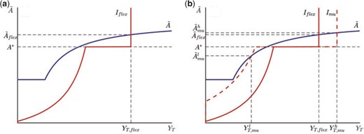
Exchange rate regime and capital flows.

Notes: Left panel: Unique equilibrium with flexible exchange rates. Right panel: Multiple equilibria in a monetary union.

Open in new tab Download slide

Imagine that under flexible exchange rates there is a unique equilibrium characterized by capital inflows toward the home country. This case is shown by Figure 1(a). As highlighted by Proposition 4, a capital inflow equilibrium exists under flexible exchange rates if |$G < (A-A^*) (N + \bar{D}_{flex}/A^*)$|⁠. Intuitively, this condition ensures that with capital inflows the tax base in the home country is large enough to guarantee that the after-tax return from investing at home is higher than the interest rate.

It is useful to pause for a second and consider why the capital flight equilibria are instead ruled out. Imagine that agents anticipate that the after-tax return from investing at home will be lower than |$A^*$|⁠. In this case, the home country will experience a capital flight. However, if foreign agents’ debt limit is tight, the capital flight will be small, and so it will have a small impact on investment, on the tax base and so on the tax rate. But then the return from investing at home will not fall below |$A^*$|⁠, contradicting the initial pessimistic expectations.³⁶ In this scenario, therefore, under flexible exchange rates expectations-driven capital flights cannot take place because international capital mobility is too low.

What might happen if the two countries adopt a common currency? A possible outcome is displayed by Figure 1(b). Once a currency union is formed financial integration increases, leading to a rise in the borrowing limits |$\bar{D}$| and |$\bar{D}^*$|⁠. Domestic agents can now sustain a higher amount of foreign debt. Hence, if |$\tilde{A} > A^*$|⁠, home agents increase their foreign borrowing and more capital is installed in the home country. Graphically, this is captured by the rightward shift in the |$I$| schedule. This implies that, if expectations coordinate on the capital inflow equilibrium, forming a monetary union leads to a more efficient international allocation of capital and to higher global production of tradable goods.

But forming a monetary union also increases the borrowing capacity of foreign agents, as captured by the leftward shift of the |$I$| schedule for |$\tilde{A} < A^*$|⁠. Now consider what happens if expectations coordinate on a capital flight equilibrium. Since the borrowing capacity of foreign agents is now higher, more capital flies out of the home country. If |$G > (A-A^*) (N - \bar{D}^*_{mu}/A^*)$|⁠, the capital flight is large enough to push the after-tax return on home investment below |$A^*$|⁠. Pessimistic expectations thus become self-fulfilling, and the capital flight indeed occurs. Forming a monetary union therefore creates the possibility of coordination failures in investment decisions. The following corollary to Proposition 4 collects these results.

Corollary 1.

Suppose that assumption 2 holds and that |$(A-A^*)(N - \bar{D}_{mu}^*/A^*)< G < (A-A^*)(N - \bar{D}_{flex}^*/A^*)$|⁠. Then under flexible exchange rates the equilibrium is unique and features capital inflows. Instead, in a monetary union there is a stable capital inflows equilibrium and at least one stable capital flight equilibrium.

In this example, the case in favour of forming a monetary union is not clear cut, and depends on expectations and animal spirits. If agents are optimistic, giving up exchange rate flexibility to join a monetary union leads to an increase in welfare, by fostering a more efficient allocation of capital across countries. However, in a monetary union self-fulfilling episodes of inefficient capital flights are possible. In particular, a wave of pessimism can induce capital flows toward the country characterized by the lowest productivity. When this happens, global production and welfare drop.

This example illustrates one of the potential dangers of forming a monetary union. The easiness with which capital can flow across countries in a monetary union, in fact, can generate financial instability and capital misallocation. Moreover, inefficient capital flights are more likely to happen when a monetary union is hit by large shocks requiring a fiscal response, such as during the ongoing Covid-19 pandemic. In this respect, the model suggests that participating in a common currency might hamper national governments’ ability to react to shocks through fiscal policy. This is the case because, due to high capital mobility, a large increase in government expenditure creates the conditions for capital flights driven by pessimistic animal spirits.³⁷

5. Policy Implications

A natural question to ask is whether there exist policy interventions that can rule out capital flight equilibria, so as to ensure that increasing financial integration by forming a monetary union leads to a rise in the union’s welfare. I will now show that several policies can accomplish this objective. But I also argue that implementing them, due to their distributive implications, might require a high degree of international cooperation.

5.1. Capital controls and fiscal transfers

Let us start by considering capital controls. Suppose that the home government can impose a limit to lending abroad by home agents. During a capital flight, home investment is given by

$$ \begin{equation}\label{theta} I = N - \min\left(\frac{\bar{D}^*}{\tilde{A}}, \theta\right)\!, \end{equation}$$

(15)

where |$\theta$| denotes the upper limit on lending to foreign agents imposed by the home government. Effectively, by managing |$\theta$| the government can impose a floor on investment in domestic capital. As illustrated by Figure 2, by setting |$\theta$| low enough the government coordinates expectations on the capital inflow equilibrium.³⁸ Intuitively, capital flight equilibria are possible only if pessimistic expectations trigger large falls in domestic investment. Controls on capital outflows rule out capital flight equilibria, by reducing the sensitivity of investment to changes in expectations.

Figure 2

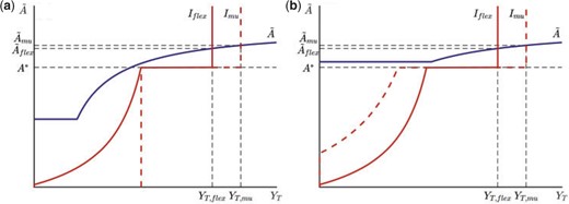
Managing capital flows in a monetary union.

Notes: Left panel: Capital controls. Right panel: Fiscal transfers.

Open in new tab Download slide

In practice, however, imposing controls on capital outflows might be challenging. The reason is that private agents have strong incentives to elude them. Ultimately, whether a government can successfully implement controls on outflows is an empirical question. While the jury is still out, existing evidence suggests that controlling capital outflows is a complicated task. For instance, Edwards (1999) summarizes the experience of emerging markets with controls on outflows, and concludes that they had a very limited impact on actual flows. Moreover, due to the complexity of their financial systems, successfully implementing controls on outflows in advanced economies might represent an even bigger challenge. In fact, Ilzetzki et al. (2019) document that controls on capital outflows have essentially been absent in advanced economies since the early 1990s.³⁹

Another possibility is to rule out capital flight equilibria through fiscal transfers. This resonates with the idea that monetary unions need to be complemented with fiscal solidarity (Kenen, 1969; Farhi and Werning, 2017). To see this point, suppose that in period 1 the foreign government makes a transfer |$T$| to the home government. The home government budget constraint then becomes

$$ \begin{equation*} G = \tau Y_T + T. \end{equation*}$$

Let us also assume that the transfer is indexed to home production of tradable goods, according to the function |$T=\max\left(G-\tilde{\tau} Y_T, 0\right)$|⁠. This policy effectively imposes an upper bound on the capital tax equal to |$\tilde{\tau}$|⁠. As long as |$A(1-\tilde{\tau}) > A^*$|⁠, capital flight equilibria are ruled out. The reason is that, as shown by Figure 2(b), with this policy in place the return to investment at home never falls below the foreign one.

So a system of sufficiently strong countercyclical transfers eliminates inefficient capital flights, by anchoring expectations on the good equilibrium in which capital flows toward high-productivity countries. Notice that, as long as the transfer scheme is credible, inefficient capital flights are ruled out without the need to actually transfer resources across countries in equilibrium. Aside from the benefits already highlighted by the literature, complementing a monetary union with a system of fiscal transfers has thus the additional advantage of preventing episodes of capital flights driven by pessimistic animal spirits.

5.2. The importance of international cooperation

There is, however, a fundamental problem with the policies proposed above. The foreign government, in fact, has an incentive to oppose them. The reason is that capital flights out of the home country increase foreign citizens’ welfare. This happens because capital flights depress the interest rate, allowing foreign agents to profit from the spread between the interest rate and the return to investment. More formally, under Assumption 2, in a capital inflows equilibrium foreign agents’ consumption of tradable goods is equal to |$A^* N^*$|⁠. Instead, in a capital flight equilibrium foreign households tradable consumption is |$A^* N^* + (A^*/\tilde{A} - 1)\bar{D}^* > A^* N^*$|⁠, since in a capital flight equilibrium |$\tilde{A} < A^*$|⁠. Hence, from a global perspective implementing policies that rule out capital flight equilibria makes sense. But these policies have important redistributive implications, and so not all countries might support them.⁴⁰

The general lesson here is that there are several policies that can eliminate episodes of self-fulfilling capital flights. Implementing them, however, might be difficult due to their distributive implications. Indeed, during episodes of inefficient capital flights, some countries—which can be thought of as safe-haven countries—benefit from inflows of cheap foreign capital. Safe-haven countries might then end up loosing from policies that anchor expectations on the equilibrium that maximizes global welfare. This result suggests that successfully managing the high degree of capital mobility characterizing monetary unions requires close cooperation among member countries.

6. Conclusion

We have thus seen that forming a monetary union is likely to lead to an increase financial integration across member countries. With a single currency, the reason is, national governments cannot use monetary policy to expropriate foreign investors. However, boosting financial integration by forming a monetary union might have an ambiguous impact on welfare. This happens because high capital mobility opens the door to episodes of expectation-driven inefficient capital flights, especially during periods of large asymmetric fiscal shocks. While there are several policies that can eliminate pessimistic equilibria, most notably countercyclical fiscal transfers, their implementation requires international cooperation because of their redistributive implications.

This article represents a first step of a larger research program connecting the exchange rate regime to financial integration. To conclude, let me mention three questions that could be addressed in future research. The first one is about boom-bust cycles in capital flows. The model suggests that countries with low net worth positions are particularly vulnerable to episodes of capital flights driven by animal spirits. According to Proposition 4, in fact, capital flights out of the home country can materialize only if |$N$| is low enough. The interesting point here is that a low |$N$| might be the result of legacy external debt. In this case, a period of large capital inflows—if it leads to a deterioration of national net worth—might create the conditions for future financial instability. This reasoning hints at the possibility that monetary unions might be particularly vulnerable to boom–bust cycles in capital flows driven by animal spirits. To investigate this hypothesis, one would need to extend the model to a fully dynamic setting, which is a very exciting topic for future research.

The second one is motivated by the fact that, in the run up to the 2008 global financial crisis, capital flows toward peripheral euro area countries were associated with a slowdown in productivity growth. Several explanations have been advanced by the literature. Benigno and Fornaro (2014) show that capital inflows might lead to lower productivity growth by discouraging innovation activities by firms in the tradable sector.⁴¹ In Gopinath et al. (2017) and Reis (2013), instead, capital inflows depress productivity by inducing misallocation of capital across firms. This literature thus suggests that capital inflows might be detrimental to productivity growth. It would be interesting to revisit the benefits and costs from forming a currency union in light of this insight.

Third, in this article, I have focused on the impact of financial integration on net capital flows and on the international allocation of capital. International financial integration, however, also affects risk sharing across countries. In this respect, the model in this paper suggests that forming a currency union might facilitate international risk sharing, by increasing the potential for gross capital flows across member countries. Investigating the relationship between the exchange rate regime, gross capital flows and international risk sharing is a promising area for future research.

The editor in charge of this paper was Veronica Guerrieri.

APPENDIX

A. Proofs

A.1. Proof of Proposition 1

Proposition 1.

Under flexible exchange rates, default does not occur if and only if |$D \leq \bar{D}_{flex}$|⁠. Moreover, in absence of default monetary policy sets |$p = Y_N = 1$|⁠. Analogous expressions hold for the foreign country.

Proof.

The home government chooses |$p$|⁠, |$Y_N$| and |$C_T$| to maximize home households’ utility

$$ \begin{equation} C_T + \frac{Y_N^{1-\eta}}{1-\eta} - Y_N, \end{equation}$$

(A.1)

subject to

$$ \begin{equation} Y_N = p^{-\frac{1}{\eta}} \end{equation}$$

(A.2)

$$ \begin{equation} C_T = Y_T - \min \left[ D, \kappa \left(Y_T + p^{1-\frac{1}{\eta}}\right) \right]\!. \end{equation}$$

(A.3)

Substituting the constraints in the objective function, the government problem reduces to choosing |$p$| to maximize

$$ \begin{equation} Y_T - \min \left[ D, \kappa \left(Y_T + p^{1-\frac{1}{\eta}}\right) \right] + \frac{p^{1-\frac{1}{\eta}}}{1-\eta} - p^{-\frac{1}{\eta}}. \end{equation}$$

(A.4)

Let us start by assuming that |$D \leq \kappa \left(Y_T + p^{1-\frac{1}{\eta}}\right)$|⁠, so that default does not occur. In this case, the objective function is maximized by setting

$$ \begin{equation} p = Y_N = 1 \equiv p_{nd}. \end{equation}$$

(A.5)

A necessary condition for this to be an equilibrium is |$D \leq \kappa \left(Y_T + 1\right)$|⁠.

Now turn to the case |$D > \kappa \left(Y_T + p^{1-\frac{1}{\eta}}\right)$|⁠, so that home households default. In this case, the objective function is maximized by setting

$$ \begin{equation} p = \left(1 + \kappa (\eta - 1)\right)^{-1} \equiv p_d. \end{equation}$$

(A.6)

A necessary condition for this to be an equilibrium is |$D > \kappa \left(Y_T + \left(1 + \kappa (\eta - 1)\right)^{\frac{1}{\eta}-1} \right)$|⁠.

The final step consists in finding the value of |$D$| for which default is avoided. Defaulting gives higher utility compared to repaying |$D$| whenever

$$ \begin{equation} Y_T - D+ \frac{p_{nd}^{1-\frac{1}{\eta}}}{1-\eta} - p_{nd}^{-\frac{1}{\eta}} < Y_T - \kappa \left(Y_T + p_d^{1-\frac{1}{\eta}}\right)] + \frac{p_d^{1-\frac{1}{\eta}}}{1-\eta} - p_d^{-\frac{1}{\eta}} \end{equation}$$

(A.7)

After a bit of algebra, the condition above can be written as

$$ \begin{equation} D > \kappa Y_T + \frac{\eta}{\eta-1} \left[ \left( 1+ \kappa (\eta-1)\right)^{\frac{1}{\eta}}-1 \right] \equiv \bar{D}_{flex}. \end{equation}$$

(A.8)

One can show that |$\kappa \left(Y_T + \left(1 + \kappa (\eta - 1)\right)^{\frac{1}{\eta}-1} \right) < \bar{D}_{flex} < \kappa \left(Y_T + 1\right)$|⁠.⁴² It follows that default is avoided if and only if |$D \leq \bar{D}_{flex}$|⁠. The problem of the government in the foreign country is symmetric. □

A.2. Proof of Proposition 2

Proposition 2.

In a monetary union, the home country does not default if and only if |$D \leq \bar{D}_{mu}$|⁠. Moreover, monetary policy sets |$p = Y_N = 1$|⁠. Analogous expressions hold for the foreign country.

Proof.

The central bank of the union chooses |$p$|⁠, |$p^*$|⁠, |$Y_N$|⁠, |$Y_N^*$|⁠, |$C_T$|⁠, |$C_T^*$| to maximize households’ utility

$$ \begin{equation} C_T + C_T^* + \frac{Y_N^{1-\eta}}{1-\eta} + \frac{Y^*_N{}^{1-\eta}}{1-\eta} - Y_N - Y_N^*. \end{equation}$$

(A.9)

Since |$Y_N = Y_N^*$| and |$C_T + C_T^* = Y_T + Y_T^*$|⁠, the objective function can be written as

$$ \begin{equation} Y_T + Y_T^* + 2\left(\frac{Y_N^{1-\eta}}{1-\eta} - Y_N\right)\!, \end{equation}$$

(A.10)

which is maximized subject to |$Y^N = p^{\frac{1}{\eta}}$|⁠. The solution is |$p = Y_N = 1$|⁠. The home country therefore does not default if and only if

$$ \begin{equation} D \leq \kappa \left(Y_T + 1\right) \equiv \bar{D}_{mu}. \end{equation}$$

(A.11)

Analogous expressions hold for the foreign country. □

A.3. Proof of Proposition 3

Proposition 3.

Suppose that |$A > A^*$| and that assumption 1 holds. Then moving from flexible exchange rates to a monetary union produces an increase in global output of tradable goods and welfare.

Proof.

Let us start by deriving the equilibrium under flexible exchange rates. Clearly it must be that |$R \geq A^*$|⁠, otherwise demand for credit would exceed credit supply. Now suppose that |$R> A^*$|⁠. Then it must be that all the funds are invested in the home country, but Assumption 1 rule out this possibility. Then it must be that |$R=A^*$| and, again by Assumption 1, investment at home is given by

$$ \begin{equation} I = N + \frac{\bar{D}_{flex}}{A^*} < N + N^*. \end{equation}$$

(A.12)

Following the reasoning outlined above, in a monetary union it must be that

$$ \begin{equation} I = N + \min\left(\frac{\bar{D}_{mu}}{A^*}, N^*\right)\!. \end{equation}$$

(A.13)

So output of tradable goods is higher in a monetary union compared to flexible exchange rates. Since production of non-traded goods does not depend on the exchange rate regime, welfare is higher in a monetary union compared to the case of flexible exchange rates.

A.4. Proof of Proposition 4

Proposition 4.

Proof.

To prove the first part of the proposition, imagine that a capital inflows equilibrium exists. In a capital inflows equilibrium the after-tax return on home investment is higher than the interest rate. Let us guess that in this equilibrium the interest rate is equal to |$A^*$|⁠. Since home agents maximize investment in domestic capital they borrow up to the limit and so

$$ \begin{equation*} I = N + \frac{\bar{D}}{A^*} < N + N^*, \end{equation*}$$

where the inequality follows from assumption (13) and the fact that |$\bar{D}_{flex} < \bar{D}_{mu}$|⁠. The tax rate is then equal to

$$ \begin{equation*} \tau = \min\left( \frac{G}{A\left(N + \frac{\bar{D}}{A^*}\right)}, \bar{\tau}\right)\!. \end{equation*}$$

Condition |$G < (A-A^*) (N + \bar{D}/A^*)$| ensures that |$\tilde{A} > A^*$|⁠. This proves that a capital inflow equilibrium exists. To see why this equilibrium is stable, imagine that there was a slight fall in aggregate investment in domestic capital. The after-tax return to investing at home would still be higher than the interest rate, meaning that home agents would have an incentive to increase investment until the initial equilibrium is restored. We do not need to consider upward movements in aggregate investment, since the borrowing constraint rules them out.

To prove the second part of the proposition, imagine that a capital flight equilibrium exists. In a capital flight equilibrium |$\tilde{A} < A^*$|⁠. Let us guess that in this equilibrium investment in home capital is positive, and so the interest rate is equal to |$\tilde{A}$|⁠. Since home agents maximize lending to foreign agents, investment in foreign capital will be equal to

$$ \begin{equation*} I^* = N^* + \frac{\bar{D}^*}{\tilde{A}} < N + N^*, \end{equation*}$$

where the inequality follows from assumption (14) and the fact that |$\bar{D}^*_\textit{flex} < \bar{D}^*_{mu}$| and |$\tau \leq \bar{\tau}$|⁠. The tax rate is then equal to

$$ \begin{equation*} \tau = \min\left( \frac{G}{A\left(N - \frac{\bar{D}^*}{\tilde{A}}\right)}, \bar{\tau}\right)\!. \end{equation*}$$

Condition |$G > (A-A^*) (N - \bar{D}^*/A^*)$| then ensures that |$\tilde{A} < A^*$|⁠. This proves that a capital flight equilibrium exists. To prove that this equilibrium is stable, consider a slight fall in aggregate investment at home. This triggers an increase in taxes and a drop in the interest rate. In turn, the drop in the interest rate increases borrowing from foreign agents leading to an increase in capital flights and a fall in home investment. The equilibrium is stable if the fall in investment drive by capital flight is smaller than the initial deviation. A symmetric argument holds for upward deviations. Therefore, an equilibrium is stable if around the equilibrium point the |$A(1-\tau)$| schedule is flatter than the |$I$| schedule. Looking at Figure 1 one can see that if a capital flight equilibrium exists, there is always going to be a capital flight equilibrium that satisfies this property.

The third part of the proposition follows from the fact that |$(A-A^*) (N - \bar{D}^*/A^*)< (A-A^*) (N + \bar{D}/A^*)$|⁠. Finally, If multiple equilibria are possible the capital inflow equilibrium will feature the highest investment in home capital. Then the capital inflow equilibrium will also be the one with the highest global production of tradable goods. Since global production of non-tradables is the same across all the equilibria, the capital inflow equilibrium will also be the one with the highest global welfare. □

B. Multiple Equilibria with Technological Spillovers

In this Appendix, I consider a scenario in which coordination failures can happen due to the presence of technological spillovers. This is the case in the classic contributions by Bryant (1987) and Murphy et al. (1989). In these frameworks, agents can invest in two technologies, one of which is characterized by a higher return. However, investing in the high-return technology is profitable only if enough agents do so. Agents can thus coordinate on an optimistic equilibrium, in which everybody ends up adopting the high-return technology. But expectations can also coordinate on a pessimistic equilibrium, in which every agent remains stuck with the low-return inefficient technology.

To capture this idea, assume that the return on home capital depends on aggregate domestic investment

$$ \begin{equation} A = \begin{cases} A_l & \quad \text{if } I < \bar{I}\\ A_h & \quad \text{if } I \geq \bar{I}. \end{cases} \end{equation}$$

(B.1)

In words, the return to investing in domestic capital experiences an upward jump once the threshold level of aggregate investment (⁠|$\bar{I}$|⁠) is reached. This is the case if switching from a low-return to a high-return technology entails positive spillovers across agents, so that the high-return technology is profitable only if it is adopted on a large-enough scale. For simplicity, assume that the return from investing in foreign capital is constant and equal to |$A^*$|⁠. Moreover, to make things interesting, consider the case |$A_l < A^* < A_h$|⁠. Hence, investing in the home economy is efficient only if the threshold level of investment |$\bar{I}$| is reached.

Individual investment decisions now depend on expectations of aggregate investment. In particular, if agents expect that |$I \geq \bar{I}$| they anticipate that capital will yield a higher return in the home country compared to the foreign one. It will then be optimal for home households to maximize investment in domestic capital by borrowing up to the limit. Conversely, if agents expect that |$I < \bar{I}$| it will be optimal for home agents to minimize investment in domestic capital by shipping as much capital as possible abroad.

Rather than fully characterizing all the possible equilibria of this version of the model, let me provide an example in which forming a monetary union reduces welfare. Again, restrict attention to equilibria in which the borrowing limit is always binding.⁴³ Now consider a case in which the equilibrium under flexible exchange rates is as depicted in the left panel of Figure B.1.

Figure B.1

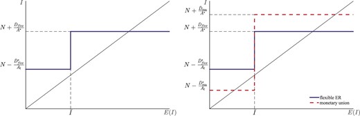
Equilibrium with aggregate increasing returns from investment.

Notes: left panel refers to flexible exchange rates, right panel shows impact of creating a monetary union.

Open in new tab Download slide

Figure B.1 plots actual investment |$I$| as a function of expected investment |$E(I)$|⁠. If |$E(I) \geq \bar{I}$| then it is more profitable to invest in home rather than in foreign capital. In this case, home agents borrow up to the limit to maximize investment in domestic capital. The equilibrium interest rate is |$R=A^*$|⁠, so that foreign agents are indifferent between investing in foreign capital or lending to home agents. If instead |$E(I) < \bar{I}$|⁠, it is foreigners who will maximize borrowing from domestic agents to invest in foreign capital. The borrowing capacity of foreign agents, however, is not large enough to fully absorb savings from home households, and so there is positive investment in home capital. The equilibrium interest rate is then |$R= A_l$|⁠, so that home agents are indifferent between investing in capital or on the credit market.

In the case shown in the figure, the only possible equilibrium is one in which investment in home-country capital is large enough so that the high-return technology is adopted. It is useful to pause for a second and consider why the pessimistic equilibrium, in which the low-return technology is adopted, is ruled out. Imagine that agents anticipate that the low-return technology will be adopted. In this case, home agents will ship capital abroad until the borrowing constraint of foreign households ends up binding. But, in the case shown in the figure, the borrowing limit of foreign agents is so tight that investment in home capital exceeds the threshold |$\bar{I}$| even if expectations coordinate on the pessimistic equilibrium. For this reason, under flexible exchange rates the pessimistic equilibrium cannot materialize.

The right panel illustrates what may happen once a monetary union is formed. Domestic agents can now sustain a higher amount of foreign debt. Hence, if the high-return technology is adopted home agents increase their foreign borrowing and more capital is be installed in the home country. Graphically, this is captured by the upward shift in the investment curve for the range |$E(I) \geq \bar{I}$|⁠. Therefore, if expectations coordinate on the optimistic equilibrium the efficiency in the international allocation of capital is higher in a monetary union compared to the case of flexible exchange rates.

But now consider what happens if agents expect that the low-return technology is adopted. Since the borrowing capacity of foreign agents is now higher, more capital flies out of the home country compared to the case of flexible exchange rates. In the case shown in the figure, this capital flight is large enough so that investment in home capital is lower than the threshold |$\bar{I}$|⁠. Hence, the low-return technology ends up being adopted, validating agents’ initial pessimistic expectations. Forming a monetary union thus creates the possibility of coordination failures in investment decisions.⁴⁴

C. Outside Investors

The model in the main text abstracts from financial flows between the monetary union and the rest of the world. This appendix revisits the analysis in Section 3, allowing agents in the monetary union to trade in financial assets with outside investors.

Imagine that there exists a third country, called rest of the world. This country does not join the monetary union, in case one is formed, but it is otherwise symmetric to the home and foreign countries considered in the main text. Denote by |$\mathcal{D}$| and |$\mathcal{D}^*$| the debt to be repaid in period 1 to investors in the rest of the world, respectively by the home and foreign country. We are interested in understanding how the presence of this external debt affects the impact of forming a monetary union on financial integration.

C.1. Flexible exchange rates

Clearly, the presence of debts toward the rest of the world does not affect in any way the analysis under flexible exchange rates. In particular, it is still the case that agents in the home country can borrow at most |$\bar{D}_\textit{flex}$| from foreign investors. The only wrinkle is that now this limit applies to the sum of loans received from investors inhabiting the foreign country and the rest of the world (i.e. default is avoided if and only if |$D+\mathcal{D} \leq \bar{D}_{flex}$|⁠). From the point of view of the home country, in fact, such flows are perfect substitutes. Likewise, the foreign country faces a ceiling on its external debt equal to |$\bar{D}^*_{flex}$|⁠. Finally, agents in the rest of the world face a borrowing limit |$\bar{D}^{\rm row}_\textit{flex}$|⁠, applying to the sum of debt owed to investors in the home and foreign countries.

C.2. Monetary union

Now turn to the case in which the home and foreign countries form a monetary union. As we will see, the interesting result here is that capital flows within the union become imperfect substitute with respect to those between the union and the rest of the world. In particular, forming a monetary union increases the borrowing capacity among member countries. But it does not affect how much the monetary union can borrow from the rest of the world, nor how much the rest of the world can borrow from the union.

As in the main text, I consider a benevolent central bank that attaches equal weight to the welfare of every citizen of the union, and that operates under discretion. I also maintain the assumption |$W=W^*$|⁠, which implies |$p = p^*$| and |$Y_N = Y_N^*$|⁠. In addition, I need to take a stance on how collateral is split between different creditors upon default. For simplicity, assume that creditors from the rest of the world are senior. This means that rest-of-the-world creditors are either repaid in full, or they appropriate all the collateral available. Luckily, the key results hold also assuming that creditors from within the union are senior, or that all creditors have the same seniority.

The problem of the union’s central bank now consists in maximizing

$$ \begin{equation*} Y_T + Y_T^* - \min\left(\mathcal{D}, \kappa(Y_T + p Y_N)\right) - \min\left(\mathcal{D}^*, \kappa(Y_T^* + p Y_N)\right) + 2 \left(\frac{Y_N^{1-\eta}}{1-\eta} - Y_N\right)\!, \end{equation*}$$

subject to

$$ \begin{equation*} Y_N = p^{-\frac{1}{\eta}}. \end{equation*}$$

As in the baseline model, the central bank has no incentives to use monetary policy to redistribute wealth between citizens of the union. This is why |$D$| and |$D^*$| do not enter the objective function of the union’s central bank. But now monetary policy can be used to reduce the payment made by citizens of the monetary union toward outside investors, and hence the presence of debt toward outside investors (⁠|$\mathcal{D}$| and |$\mathcal{D}^*$|⁠) might influence the monetary policy stance.

To solve this problem, we can follow the same strategy pursued in Section 3. The only difference is that now default might occur either in just one country of the union or in both. There are thus three cases to consider. First, if neither the home or the foreign country default, it is optimal for the central bank to replicate the natural allocation by setting |$p=1$|⁠. The second possibility is that just one member country defaults. In this partial default scenario, it is optimal for the central bank to engineer a moderate devaluation and set |$p = (1+k(\eta-1)/2)^{-1} <1$|⁠. The third case is one in which both member countries default. In this full default scenario, it is optimal to engineer a large devaluation by setting |$p = (1+k(\eta-1))^{-1}<(1+k(\eta-1)/2)^{-1}$|⁠.⁴⁵

Again following the steps described in Section 3, one can show that investors from the rest of the world are repaid in full if and only if the following conditions are satisfied

$$ \begin{equation}\label{ou1} \mathcal{D} + \mathcal{D}^* \leq \kappa(Y_T + Y_T^*) + \frac{2\eta}{\eta-1} \left(\left(1+\kappa (\eta-1)\right)^{\frac{1}{\eta}} -1\right) \equiv \bar{\mathcal{D}}^{mu} \end{equation}$$

(C.1)

$$ \begin{equation}\label{ou2} \mathcal{D} \leq \kappa Y_T + \frac{2\eta}{\eta-1} \left(\left(1+\frac{\kappa}{2} (\eta-1)\right)^{\frac{1}{\eta}} -1\right) \equiv \bar{\mathcal{D}} \end{equation}$$

(C.2)

$$ \begin{equation}\label{ou3} \mathcal{D}^* \leq \kappa Y^*_T + \frac{2\eta}{\eta-1} \left(\left(1+\frac{\kappa}{2} (\eta-1)\right)^{\frac{1}{\eta}} -1\right) \equiv \bar{\mathcal{D}}^*. \end{equation}$$

(C.3)

The first condition ensures that the aggregate debt of the union toward outside investors is small enough to avoid a full default. The second condition ensures that the debt owed by the home country toward investors from the rest of the world is small enough to prevent the home country from defaulting. The third condition ensures that the same holds for the foreign country.

Since investors from the rest of the world are rational, they will never lend a sum large enough to trigger a default. It follows that conditions (C.1)–(C.3) describe the endogenous debt ceilings imposed by investors from the rest of the world on countries member of the monetary union. Notice that the first condition can be also written as |$\mathcal{D} + \mathcal{D}^* \leq \bar{D}_\textit{flex} + \bar{D}^*_\textit{flex}$|⁠, meaning that forming a monetary union does not affect the maximum debt toward the rest of the world that the union can sustain without defaulting.

What about loans among member countries? Recall that the central bank has no incentives to redistribute wealth inside the union. Since conditions (C.1)–(C.3) are satisfied in equilibrium, the union’s central bank then sets |$p = Y_N = 1$| to replicate the allocation under flexible wages, regardless of the amount of debt that member countries owe to each other. Hence, member countries are able to borrow from investors within the union up to their full collateral value. For instance, agents in the home country are able to borrow from investors in the foreign country up to

$$ \begin{equation} D < \kappa (Y_T +1) - \mathcal{D} \equiv \bar{D}_{mu} - \mathcal{D}, \end{equation}$$

(C.4)

without triggering a default. Since |$\bar{D}_{mu} > \bar{D}_\textit{flex}$|⁠, forming a monetary union increases the total amount of external debt (i.e. |$D+\mathcal{D}$|⁠) that the home country can sustain without defaulting. The same applies to the foreign country.

Interestingly, forming a monetary union creates an endogenous segmentation in the international credit markets. Let’s once again take the perspective of the home country. After a monetary union is formed, the maximal external debt that the home country can sustain without defaulting is equal to |$\bar{D}_{mu}$|⁠. But conditions (C.1) and (C.2) imply that investors from outside the union are willing to lend to the home country at most |$\min \left(\bar{\mathcal{D}}^{mu} - \mathcal{D}^*, \bar{\mathcal{D}}\right)$|⁠, which is strictly lower than |$\bar{D}_{mu}$|⁠. Therefore, any external borrowing in excess of |$\min \left(\bar{\mathcal{D}}^{mu} - \mathcal{D}^*, \bar{\mathcal{D}}\right)$| has to be obtained from investors within the monetary union. The reason why loans from investors outside and within the union are not perfect substitutes, of course, is that the central bank of the union has an incentive to use monetary policy to expropriate outside investors, but not investors within the union.

In a similar fashion, when a country joins a currency union the potential for capital outflows increases, but only toward other members of the union. Before a monetary union is formed, for instance, home agents can lend to the foreign country at most |$\bar{D}^*_\textit{flex}$|⁠. This threshold increases to |$\bar{D}^*_{mu}$| once a monetary union is formed. But the amount that they can safely lend to the rest of the world, |$\bar{D}^{\rm row}_\textit{flex}$|⁠, is not affected by whether the home and foreign countries form a monetary union or not.

The key lesson here is that forming a monetary union increases financial integration among member countries, but not between the monetary union and the rest of the world.⁴⁶ This implication of the model squares well with the experience of the euro area, in which member countries receive the majority of their capital inflows from within the union (Gros, 2017).

D. Diminishing Returns from Consuming Tradable Goods

In this Appendix, I study an economy in which households’ utility from consuming tradable goods is subject to diminishing returns. The analysis of this case is quite complex, and this version of the model does not lend itself to the clean characterization of the baseline one. Nonetheless, even in this case it is possible to derive some analytical insights. The main result is that the presence of concave utility introduces an incentive for the central bank of the union to redistribute wealth across countries. In this respect, the model with concave utility yields similar insights to the one studied in Section 3.4.1. Here, however, the union’s central bank has an incentive to redistribute wealth toward the poorer countries of the union. The implication is that forming a monetary union has an asymmetric impact on financial integration. That is, while forming a monetary union increases the foreign borrowing capacity for all member countries, this effect is stronger for the wealthier countries of the union, and it is weaker for the poorer ones.

Suppose that the utility function of home households is

$$ \begin{equation*} \log C_T + \frac{C_N^{1-\eta}}{1-\eta} - L, \end{equation*}$$

so that the utility from consuming tradable goods is subject to diminishing returns. The utility function of foreign households is symmetric. In this case, the relative price of the non-tradable good is given by

$$ \begin{equation*} p = \frac{C_T}{Y_N^\eta}. \end{equation*}$$

Hence, keeping everything else constant, a higher consumption of tradables produces an increase in the relative price of the non-traded good. Using |$p Y_N = C_T Y_N^{1-\eta}$|⁠, consumption of tradable goods by home agents is then given by

$$ \begin{equation*} C_T = Y_T - \min\left(D, \kappa \left(Y_T + C_T Y_N^{1-\eta}\right)\right)\!. \end{equation*}$$

This expression embeds the fact that home agents default whenever collateral value is smaller than the repayment promised to creditors, i.e., when |$D > \kappa C_T Y_N^{1-\eta}$|⁠. As in the baseline model, assuming |$\eta > 1$|⁠, a higher production of non-tradables depresses |$p$| and lowers the value of collateral that creditors repossess upon default. That is why, conditional on defaulting, there is a positive relationship between |$C_T$| and |$Y_N$|⁠. Conversely, a higher |$C_T$| increases collateral value, reducing households’ disposable income in the default state.

D.1. Flexible exchange rates

Let us start by considering the case of flexible exchange rates. It is useful to write the problem of the home government as

$$ \begin{equation*} \max_{C_T, Y_N} \log C_T + \frac{Y_N^{1-\eta}}{1-\eta} - Y_N, \end{equation*}$$

subject to

$$ \begin{equation}\label{concon} C_T =Y_T - \min\left(D, \kappa \left(Y_T+ C_T Y_N^{1-\eta}\right)\right)\!. \end{equation}$$

(D.1)

Conditional on debt repayment, the solution to this problem is simply to replicate the natural allocation by setting |$Y_N = 1$|⁠. In case of default, instead, the optimality conditions are

$$ \begin{equation*} \frac{1}{C_T} = \lambda \left(1+ \kappa Y_N^{1-\eta}\right) \end{equation*}$$

$$ \begin{equation*} Y_N^{-\eta} = 1- \lambda \kappa (\eta-1) C_T Y_N^{-\eta}, \end{equation*}$$

where |$\lambda$| denotes the Lagrange multiplier on constraint (D.1). The left hand-side of the first optimality condition captures the marginal rise in welfare from increasing |$C_T$|⁠. The right-hand side, instead, captures the associated marginal cost. Intuitively, a rise of one unit of |$C_T$| requires a rise in the income of tradable goods of |$1+\kappa Y_N^{1-\eta}>1$| units, because as |$C_T$| rises so does collateral value, and hence the repayment made to creditors. The second optimality condition encapsulates the optimal choice of |$Y_N$|⁠, taking into account the impact of changes in |$Y_N$| on collateral value and hence on |$C_T$|⁠.

Combining the two optimality conditions above gives that the optimal production of non-tradable goods solves

$$ \begin{equation}\label{YNcon} Y_N^{-\eta} \left(1+\frac{\kappa (\eta-1)}{1+\kappa Y_N^{1-\eta}}\right) = 1. \end{equation}$$

(D.2)

Denoting the solution to this equation by |$Y_{N, \rm dflex}$|⁠, one can see that |$Y_{N, \rm dflex} >1$|⁠. Just as in the baseline model, in case of default the national government has an incentive to depreciate the exchange rate and push production of non-tradable goods beyond its natural level, in order to reduce collateral value and the payment made to foreign creditors. Given this result, the maximum amount of external debt that the home country can sustain without defaulting |$\bar{D}_\textit{flex}$| is implicitly defined by

$$ \begin{equation}\label{Dflexcon} \log\left(Y_T - \bar{D}_{flex}\right) - \frac{\eta}{\eta-1} = \log\left(\frac{(1-\kappa)Y_T}{1+\kappa Y_{N, \rm dflex}^{1-\eta}}\right) + \left(\frac{Y_{N, \rm dflex}^{1-\eta}}{1-\eta} - Y_{N, \rm dflex}\right)\!. \end{equation}$$

(D.3)

D.2. Monetary union

Solving the model in the case of a monetary union is, unfortunately, much more complex. Rather than fully characterizing the solution to this version of the model, a task that I leave for future research, here I would like to highlight an interesting insight. For this reason, I will make a simplifying assumption. Let us consider a case in which the home country is a debtor and the foreign one is a creditor. From now on, I will assume that wages in the creditor country are flexible. This assumption implies that output of non-tradable goods in the foreign country is always at its natural level, so that |$Y_N^* = 1$|⁠.⁴⁷

The maximization problem of the union’s central bank can then be written as

$$ \begin{equation*} \max_{C_T, C_T^*, Y_N} \log C_T + \log C_T^* + \frac{Y_N^{1-\eta}}{1-\eta} - Y_N \end{equation*}$$

subject to

$$ \begin{gather}\label{concon1} C_T = Y_T - \min\left(D, \kappa \left(Y_T + C_T Y_N^{1-\eta}\right)\right)\\ \end{gather}$$

(D.4)

$$ \begin{gather} C_T^* = Y_T + Y_T^* - C_T. \end{gather}$$

(D.5)

Conditional on debt repayment by the home country, it is optimal for the central bank to replicate the natural allocation by setting |$Y_N = 1$|⁠. In case of default, instead, the optimality conditions are

$$ \begin{gather*} \frac{1}{C_T} - \frac{1}{C_T^*} = \lambda_{mu} \left(1+ \kappa Y_N^{1-\eta}\right)\\ Y_N^{-\eta} = 1 - \lambda_{mu} (\eta-1) \kappa C_T Y_N^{-\eta}, \end{gather*}$$

where |$\lambda_{mu}$| denotes the Lagrange multiplier on constraint (D.4). The intuition behind these optimality conditions follows closely the one for the optimality conditions under flexible exchange rates. There is, however, one important difference. In fact, now the impact on welfare of a marginal rise in |$C_T$|—captured by the left-hand side of the first optimality condition—is equal to |$1/C_T - 1/C_T^*$|⁠. The reason is that a rise in |$C_T$| is associated with an equivalent drop in |$C_T^*$|⁠. The ratio |$C_T/C_T^*$| determines whether this has a positive or negative impact on the aggregate welfare of the union. If |$C_T < C_T^*$| then redistributing tradable consumption toward the home country leads to a rise in welfare, while the opposite occurs if |$C_T>C_T^*$|⁠. Hence, the central bank of the union has a motive to redistribute wealth toward the poorer member countries.

Combining the two optimality conditions gives

$$ \begin{equation}\label{dan} Y_N^{-\eta} \left(1+ \left(1-\frac{C_T}{C_T^*}\right) \frac{\kappa (\eta-1)}{1+\kappa Y_N^{1-\eta}}\right) = 1. \end{equation}$$

(D.6)

This equation implies that—conditional on the home country defaulting—|$Y_N$| is decreasing in |$C_T/C_T^*$|⁠. The reason is simple. A lower ratio |$C_T/C_T^*$| magnifies the union’s central bank incentive to expropriate foreign creditors so as to increase consumption by home agents. So if |$C_T = C_T^*$| it is optimal for the central bank to set |$Y_N=1$|⁠, because redistributing wealth across the two countries would not change the aggregate utility of the union. If |$C_T > C_T^*$|⁠, then the central bank sets |$Y_N<1$|⁠, because doing so boosts collateral value and redistributes wealth toward the poorer country, that is the creditor one. Finally, if |$C_T<C_T^*$| then the central bank sets |$Y_N>1$|⁠, so as to dilute collateral value and redistribute wealth toward the debtor country, which is now poorer than the creditor one.

Moreover, comparing (D.6) with (D.2), one can see that in case of default the union’s central bank will always choose a lower |$Y_N$| compared to the national government of the home country. Intuitively, the union’s central bank has a weaker incentive to dilute collateral and expropriate creditors, because creditors’ welfare enters its objective function. Therefore, as in the baseline model, the incentive to use monetary policy to expropriate creditors is always weaker in a currency union compared to the case of flexible exchange rates.

Using the market clearing conditions for |$C_T$| and |$C_T^*$|⁠, one can rewrite the optimality condition for |$Y_N$| as

$$ \begin{equation*} Y_N^{-\eta} \left(1+ \left(1-\frac{(1-\kappa) Y_T}{(Y_T+ Y_T^*)(1+\kappa Y_N^{1-\eta}) - (1-\kappa)Y_T}\right)\frac{\kappa (\eta-1)}{1+\kappa Y_N^{1-\eta}}\right) = 1. \end{equation*}$$

Denote the solution to this equation by |$Y_{N, dmu}$|⁠. The maximum amount of external debt that the home country can sustain without defaulting |$\bar{D}_{mu}$| is implicitly defined by

$$ \begin{equation}\label{Dmucon} \log\left(Y_T - \bar{D}_{mu}\right) - \frac{\eta}{\eta-1} = \log\left(\frac{(1-\kappa)Y_T}{1+\kappa Y_{N, dmu}^{1-\eta}}\right) +\frac{Y_{N, dmu}^{1-\eta}}{1-\eta} - Y_{N, dmu} + \log\left( \frac{C_{T, dmu}^*}{Y^*_T + \bar{D}_{mu}}\right), \end{equation}$$

(D.7)

where |$C_{T, dmu}^*$| denotes consumption of tradable goods by the foreign country conditional on default by the home country, which is equal to

$$ \begin{equation*} C_{T, dmu}^* \equiv Y_T^*+\frac{\kappa Y_T\left(1+Y_{N,dmu}^{1-\eta}\right)}{1+\kappa Y_{N, dmu}^{1-\eta}}. \end{equation*}$$

D.3. Impact of forming a monetary union on financial integration

We are now ready to derive the impact on financial integration from forming a currency union. Comparing (D.3) and (D.7) one can see that |$\bar{D}_{mu}>\bar{D}_\textit{flex}$| if

$$ \begin{equation*} \log\left(\frac{(1-\kappa)Y_T}{1+\kappa Y_{N, \rm dflex}^{1-\eta}}\right) + \frac{Y_{N, \rm dflex}^{1-\eta}}{1-\eta} - Y_{N, \rm dflex} > \log\left(\frac{(1-\kappa)Y_T}{1+\kappa Y_{N, dmu}^{1-\eta}}\right) +\frac{Y_{N, dmu}^{1-\eta}}{1-\eta} - Y_{N, dmu} + \log\left( \frac{C_{T, dmu}^*}{Y^*_T + \bar{D}_{mu}}\right)\!. \end{equation*}$$

This inequality always holds (as long as |$Y_T^*<+\infty$|⁠).⁴⁸ Therefore, the first result is that forming a monetary union always has a positive impact on financial integration.

Another interesting insight is that quantitatively the impact of forming a monetary union on financial integration depends on the relative wealth of the two countries. This is best seen by considering how |$\bar{D}_{mu}$| varies as |$Y_T^*$| changes. First, consider that if |$Y_T^*\rightarrow +\infty$| then |$\bar{D}_{mu} \rightarrow \bar{D}_\textit{flex}$|⁠.⁴⁹ This corresponds to a scenario in which the creditor country is extremely wealthy compared to the debtor one, and so the union’s central bank has a very strong incentive to use monetary policy to expropriate creditors. This effect explains why moving from flexible exchange rates to a monetary union has only a marginal impact on the credit ceiling imposed by foreign investors on the home country.

Second, one can show that |$\bar{D}_{mu}$| is decreasing in |$Y_T^*$|⁠.⁵⁰ This means that as the creditor country gets poorer the temptation of the union’s central bank to dilute collateral to expropriate creditors gets weaker, and the maximum amount of foreign debt that the home country can sustain rises. This result points toward an asymmetric impact of forming a monetary union on financial integration. Since the incentives to expropriate are weaker when the borrower is relatively rich, forming a monetary union relaxes more the borrowing limit for rich countries, compared to poor ones.

Acknowledgments

I thank the Editor, Veronica Guerrieri, three anonymous referees, Daria Finocchiaro, Jeffry Frieden, Pierre-Olivier Gourinchas, Matteo Maggiori, Tommaso Monacelli, Dmitry Mukhin, Julia Oliva, Luis Rojas, Dmitriy Sergeyev, Olivier Wang, and seminar/conference participants at CREI, the Oxford/New York Fed Monetary Economics Conference, Université Catholique de Louvain, University of Vienna, the CEPR IMF Programme meeting, Università Bocconi, ETLA, the ADEMU workshop on A Dynamic Economic and Monetary Union, IMF, University of Wisconsin and Columbia University for very helpful comments. Andrea Chiavari, Lauri Esala, and Luigi Falasconi provided excellent research assistance. Financial support from the European Research Council under the European Union’s Horizon 2020 research and innovation program, Starting Grant (851896-KEYNESGROWTH) and the Spanish Ministry of Economy and Competitiveness, through the Severo Ochoa Programme for Centres of Excellence in R&D (SEV2015-0563 and CEX2019-000915-S), and from the Generalitat de Catalunya, through CERCA and SGR Programme (2017-SGR-1393), is gratefully acknowledged. An earlier version of this paper has circulated under the title “Monetary Union and Financial Integration.”

Footnotes

In fact, euro area peripheral countries enjoyed large capital inflows after adopting the euro, which were then followed by sharp capital flights in the aftermath of the 2008 global financial crisis (Lane, 2012; Shambaugh, 2012; Fornaro, 2018). Interestingly, Keynes anticipated that currency unions, due to their high degree of capital mobility, could be particularly prone to financial instability and volatility in capital flows (see Keynes, 1930, Chapter 36). This reasoning made him skeptic of the notion that increasing financial integration by forming a monetary union would necessarily have a positive impact on welfare.

Pegging the exchange rate, conversely, does not help mitigating the time-consistency problem studied by the literature on nominal debt, since real or foreign currency debt can be issued even under flexible exchange rates. See Araujo et al. (2013), Engel and Park (2018), and Ottonello and Perez (2019) for some recent examples of the literature on domestic currency debt and limited commitment over monetary policy.

The expression vincolo esterno—meaning external constraint in Italian—was introduced by Italian policymakers during the negotiations leading to the Maastricht treaty (Dyson and Featherstone, 1999). Back then, it was a widespread belief among Italian policymakers that the euro would carry a desirable external constraint on domestic policy. In the model, I capture this notion by assuming that member countries commit not to exit the monetary union. Alternatively, one could allow countries to exit the union upon paying an exit cost. This alternative assumption would not alter substantially the results of the article.

The union’s central bank, instead, has an incentive to expropriate creditors from outside the monetary union. For this reason, the model predicts that forming a monetary union should increase financial integration among member countries, while leaving largely unaffected capital mobility between the union and the rest of the world. This result helps explain why euro area countries receive the majority of their capital inflows from within the union (Gros, 2017).

The reason is that the presence of taxes on capital gives rise to private increasing returns to investment. In fact, the main results of the article would go through as long as the private return to investment is increasing in aggregate investment. For instance, in Appendix B, I study a version of the model in which investment complementarities arise from the presence of technological spillovers across firms.

Araujo et al. (2013) and Corsetti and Dedola (2016) show that countries with fixed exchange rates are particularly prone to experience self-fulfilling runs on sovereign debt, of the type first studied by Cole and Kehoe (2000). The underlying logic is that fixed exchange rates prevent the monetary authority from ruling out self-fulfilling crises by making the real value of domestic-currency debt state contingent. The reason why monetary unions are exposed to the risk of self-fulfilling crises in this article is very different. Here, in fact, forming a monetary union might give rise to multiple equilibria because it increases capital mobility among member countries.

In a very interesting recent paper, Itskhoki and Mukhin (2021) study a framework in which pegging the exchange rate leads to higher financial integration. Similar to Doepke and Schneider (2017), in Itskhoki and Mukhin (2021) the exchange rate regime affects financial integration because households are allowed to trade in domestic currency bonds only, and international financial intermediaries have limited arbitrage capacity. Moreover, also in Itskhoki and Mukhin (2021) central banks follow simple rules, and the optimal monetary policy is not considered.

The assumption that utility is linear in consumption of the tradable good is key in order to solve the model analytically (Appendix D considers the case of concave utility). Instead, the assumption that disutility from labour effort is linear is made purely to simplify notation and could be easily relaxed.

Notice that here, in line with the sovereign default literature and with Kiyotaki and Moore (1997), collateral is provided by the household’s income in the period in which debt repayment is due. Another possibility, first explored by Mendoza (2002), is to assume that collateral is given by the household’s income in the period in which the debt contract is signed. As long as the monetary authority acts after the credit contracts are signed, the key results of the paper would hold true also under this alternative financial friction.

10.

Assuming a constant elasticity of substitution aggregator for consumption, |$\eta$| would capture the elasticity of substitution between tradable and non-tradable goods. As discussed by Ottonello (2021), the empirical evidence points toward values of |$\eta$| greater than one.

11.

Imagine that in period 1 the monetary authority in the home country sets the money supply |$M$|⁠. Now suppose that households need money to purchase consumption goods, so that

$$ \begin{equation*} P_T C_T + P_N C_N = M.\end{equation*}$$

Using (4), (5), and (8), the expression above can be written as

$$ \begin{equation*} P_T \left(Y_T - \min \left[D, \kappa \left(Y_T + W^{1-\frac{1}{\eta}} P_T^{\frac{1}{\eta}}\right)\right] \right)+ W^{1-\frac{1}{\eta}} P_T^{\frac{1}{\eta}} = M.\end{equation*}$$

Since |$Y_T, D,$| and |$W$| are all predetermined in period 1, by setting |$M$| the monetary authority controls |$P_T$|⁠.

12.

See Appendix A.1 for a detailed derivation of the solution to the government problem.

13.

In fact, notice that when |$Y_N=1$| the marginal utility of non-tradable consumption (⁠|$Y_N^{-\eta}$|⁠) and the marginal disutility from working (⁠|$1)$| are equalized.

14.

Appendix A contains all the proofs.

15.

Foreign creditors impose the borrowing limit |$D\leq \bar{D}_\textit{flex}$| on each individual household because I focus on symmetric equilibria, in which every household is treated equally. In Section 3.4.3 I briefly discuss asymmetric equilibria, in which creditors enforce the foreign debt ceiling through rationing.

16.

Obstfeld and Rogoff (1996) show that a similar result applies when the return from investment in physical capital is used as collateral, and agents decide their investment strategy after credit contracts are signed (see Chapter 6, Section 2). In their setting, debtors have an incentive to reduce investment in order to decrease the value of collateral, and thus the resources that creditors repossess in case of default. This implies that a small increase in debt can trigger a discrete fall in investment and collateral value.

17.

Ottonello (2021) studies the optimal monetary policy under commitment in an economy in which, as in this paper, creditors repossess a fraction of the country’s income upon default. He finds that the debt ceiling imposed by foreign investors coincides with the equilibrium value of collateral.

18.

In accordance with most of the literature on monetary unions, I assume that exiting the union is prohibitively costly, so that countries can credibly commit to their participation. It would not be hard to extend the analysis to cases in which exit costs are finite.

19.

In Section 3.4.1, I consider how the presence of redistributive motives affect the behaviour of the union’s central bank.

20.

With |$W\neq W^*$|⁠, it would not be possible for the central bank of the union to replicate the natural allocation. In this case, up to a first-order approximation, the optimal monetary policy would be such that |$(Y_N + Y_N^*)/2 = 1$| (see Benigno (2004) for a derivation of an analogous result in the standard New-Keynesian open-economy model). The optimal monetary policy would thus essentially eliminate the impact of nominal rigidities on the aggregate output of the union. Still, the central bank of the union would have no incentives to affect the value of collateral in order to redistribute wealth across the two countries.

21.

To be precise, forming a monetary union does not completely solve the time-consistency problem. In fact, in period 0 the central bank of the union might have an incentive to promise a deviation of output from its natural level in period 1, so as to increase collateral value. When period 1 comes, however, it will be optimal for the central bank to renege on its past promises, and to replicate the natural allocation.

22.

This contrasts with the models studied by Fornaro (2015) and Ottonello (2021). There changes in the exchange rate regime affect international borrowing constraints precisely because they have an impact on the real exchange rate and on collateral value in equilibrium. This difference is due to the fact that Fornaro (2015) and Ottonello (2021) consider national governments that operate under commitment.

23.

Here I am assuming that the union’s central bank, perhaps for political reasons, deviates from the objective function of a benevolent planner that maximizes the sum of all agents’ utilities. Another possibility is to introduce heterogeneity in the utility that agents derive from the consumption of tradable goods. If the utility that home (foreign) agents derive from the consumption of tradable goods is equal to |$\xi C_T$| (⁠|$(1-\xi) C_T^*$|⁠), then the objective function considered in this section corresponds to the one of a benevolent planner seeking to maximize the sum of all agents’ utilities. As long as |$W$| and |$W^*$| are such that |$Y_N = Y_N^*$|⁠, all the results below apply also to this case.

24.

See the proof to Proposition 1.

25.

To prove that the debt ceiling implied by (11) is higher than |$\bar{D}_\textit{flex}$|⁠, start by observing that it is decreasing in |$\xi$|⁠, and that |$\xi$| reaches its maximum at 1. It is then sufficient to prove that

$$ \begin{equation*} 2\left( (1+\frac{\kappa}{2} (\eta-1))^{\frac{1}{\eta}}-1\right) - \left( (1+\kappa (\eta-1))^{\frac{1}{\eta}}-1\right)>0.\end{equation*}$$

The expression above holds as an equality for |$\kappa=0$| and it is increasing in |$\kappa$|⁠, which completes the proof.

26.

This is not visible in the baseline model, which focuses on symmetric equilibria in which every borrower is treated equally. But foreign creditors may enforce the aggregate debt ceiling through rationing. That is, they could allow some domestic agents to borrow up to |$\kappa(Y_T +1 )$|⁠, while denying access to credit to the rest.

27.

To be sure, some changes in financial regulation might be geared toward facilitating flows within the union. But most legal reforms aiming at increasing protection of creditors’ rights do not discriminate on the base of the creditors’ nationality.

28.

In accordance with most of the literature, here I assume that households can commit to an investment plan designed before credit contracts are signed. See Obstfeld and Rogoff (1996) (Chapter 6, Section 2) for a discussion of this assumption.

29.

Gourinchas and Jeanne (2006) find that the welfare gains strictly related to a better allocation of physical capital across countries are small, especially if compared to the welfare gains from increasing productivity. However, it is not hard to think of channels through which higher financial integration can lead to an increase in total factor productivity. For instance, as in Howitt and Aghion (1998), one could assume that investment in physical capital and innovation are complements. In Gourinchas and Jeanne (2005), instead, inflows of foreign capital can induce the government to implement reforms aiming at increasing productivity.

30.

Formally, this is captured by the conditions stated in assumption 1, which hold for sufficiently low values of |$\kappa$|⁠.

31.

See, for instance, Chapter 2 of the October 2012 edition of the IMF Global Financial Stability Report.

32.

To be clear, the results presented below do not restrict themselves to the case of fiscal externalities. In fact, one can think of many other sources of coordination failures in investment decisions that would lead to similar results. For instance, in Appendix B, I consider a setting in which increasing returns in investment arise from technological spillovers. Another possibility, following Gourinchas and Jeanne (2005), is to consider a case in which the return from investment depends on some productivity-enhancing reform that the government might implement after investment decisions are taken.

33.

There are thus some similarities with Lamont (1995), who shows that private debt overhang can give rise to equilibrium multiplicity by inducing agents to make socially inefficient investment decisions.

34.

For instance, imagine that the government had to finance its expenditure by taxing deposits in the domestic banking sector, without being able to tax deposits held abroad by domestic agents.

35.

This assumption is required to rule out an extreme equilibrium in which agents anticipate a 100% tax on capital, inducing them to completely avoid investing in the home country. Alternatively, one could rule out this extreme equilibrium by assuming that investment in capital is irreversible, and that the home country enters period 0 with some pre-installed capital.

36.

Formally, this is the case if |$G < (A-A^*) (N - \bar{D}^*_\textit{flex}/A^*)$|⁠.

37.

These results also apply to other sources of high capital mobility. For instance, following Section 3.4.3, consider financial reforms leading to an increase in |$\kappa$| and |$\kappa^*$|⁠. Graphically, the impact of these reforms looks exactly like the movement from flexible exchange rates to a monetary union as illustrated by Figure 1. Therefore, also legal reforms aiming at achieving higher financial integration can open the door to multiple equilibria and inefficient capital flows. This is an application of the general insight that partially relaxing financial frictions in economies with market incompleteness might have an ambiguous impact on welfare.

38.

More precisely, in order to rule out capital flight equilibria |$\theta$| must be such that |$G < (A-A^*) (N - \theta)$|⁠.

39.

That said, recently controls on outflows have been imposed inside the euro area by Cyprus (Michaelides, 2014) and Greece. Moreover, Benediktsdottir et al. (2017) argue that in Iceland controls on outflows were successful in mitigating capital flights in the aftermath of the 2008 financial crisis.

40.

Matters would be even more complex with within-country heterogeneity. For instance, imagine that foreign agents are split between productive agents and savers. The income of productive agents is increasing in investment in foreign capital, either because they directly own capital or because they supply some factor of production (for instance land or labour) whose return is increasing in the capital stock. Savers, instead, can only earn income by lending their savings on the credit markets. In this case, foreign productive agents would gain from an episode of capital flight out of the home country. But savers would lose, because they would enjoy a lower return on their savings.

41.

42.

To prove the left part of the inequality, consider that it can be written as

$$ \begin{equation*} \eta \left( x^{\frac{1}{\eta}} - 1 \right) > \left(1-\frac{1}{x}\right) x^{\frac{1}{\eta}}, \end{equation*}$$

where |$x \equiv 1 +\kappa (\eta-1) > 1$|⁠. Rearranging gives

$$ \begin{equation*} x^{\frac{1}{\eta}} \left(\eta - 1 +\frac{1}{x}\right) > \eta.\end{equation*}$$

To complete the proof, notice that the left-hand side is increasing in |$x$| for |$x>1$| and the expression holds as an equality if |$x=1$|⁠. To prove the right part of the inequality, consider that it can be written as

$$ \begin{equation*} \eta x^{\frac{1}{\eta}} - x < \eta - 1.\end{equation*}$$

To complete the proof, notice that the left-hand side is decreasing in |$x$| for |$x>1$| and the expression holds as an equality if |$x=1$|⁠.

43.

This requires that |$N$| and |$N^*$| are sufficiently large.

44.

There are some similarities with the results highlighted by Bryant (1987). In Bryant’s model agents can invest in capital, which is characterized by increasing aggregate returns, and cash, which offers a fixed return. The option to invest in cash makes it possible for agents to coordinate on pessimistic equilibria in which the increasing returns from investing in capital are not exploited. The key difference is that in the model of this article the exchange rate regime determines the extent to which agents can divert their savings away from investment in domestic capital, and thus whether multiple equilibria are possible.

45.

Intuitively, the marginal gain from lowering |$p$| below 1 is increasing in the number of member countries that default on their debts toward outside investors. Instead, the marginal cost, given by the distortion in the production of non-tradable goods, does not depend on how many member countries default. This explains why the optimal |$p$| is lower in the full default scenario, compared to the partial default one.

46.

A caveat is in order. Condition (C.1) implies that forming a monetary union does not change the maximal amount of external debt that the monetary union as a whole can take. But conditions (C.2) and (C.3) imply that, after a monetary union is formed, individual countries might increase their borrowing from outside the union (since |$\bar{\mathcal{D}} > \bar{D}_\textit{flex}$| and |$\bar{\mathcal{D}}^* > \bar{D}^*_\textit{flex}$|⁠). In any case, forming a monetary union always has a larger impact on borrowing capacity from investors within the union (since |$\bar{\mathcal{D}} < \bar{D}_{mu}$| and |$\bar{\mathcal{D}}^* <\bar{D}^*_{mu})$|⁠.

47.

Alternatively, I could have assumed that the government in the foreign country, or even the central bank of the union, is endowed with enough fiscal instruments to determine |$Y_N^*$| independently of the monetary stance chosen by the central bank of the union. In fact, in the analysis that follows it would be optimal for the foreign government, as well as for the union’s central bank, to set |$Y_N^*=1$| if it could be chosen independently of |$Y_N$|⁠. See Farhi et al. (2014) for an analysis of the fiscal instruments needed to replicate the impact of nominal devaluations in a monetary union.

48.

To see this, consider that |$C_{T, dmu}^*/(Y^*_T +\bar{D}_{mu})<1$|⁠, since debtors default only if this reduces creditors’ consumption. Moreover, |$Y_{N,\rm dlfex}$| is precisely the value of |$Y_N$| that maximizes the term

$$ \begin{equation*} \log\left(\frac{(1-\kappa)Y_T}{1+\kappa Y_{N}^{1-\eta}}\right) + \frac{Y_{N}^{1-\eta}}{1-\eta} - Y_{N}.\end{equation*}$$

49.

Consider that if |$Y_T^*\rightarrow +\infty$| then |$C_T/C_T^*\rightarrow 0$|⁠, and so |$Y_{N,dmu} \rightarrow Y_{N,\rm dflex}$|⁠. Moreover, |$Y_T^*\rightarrow +\infty$| implies |$C_{T, dmu}^* /(Y_T^* + \bar{D}_{mu} ) \rightarrow 1$|⁠.

50.

The proof is by contradiction. Imagine that instead |$\bar{D}_{mu}$| is increasing in |$Y_T^*$|⁠. For this to happen, the right-hand side of (D.7) must be decreasing in |$Y_T^*$|⁠. First consider that a fall in |$Y_T^*$| is associated with a drop in |$C_T^*/C_T$| and, by (D.6), with a fall in |$Y_{N,dmu}$|⁠. Since the first three terms on the right-hand side of (D.7) reach their maximum when |$Y_N= Y_{N, \rm dflex}$|⁠, and since by (D.6) |$Y_{N,dmu}<Y_{N, \rm dflex}$|⁠, then a fall in |$Y_T^*$| leads to a drop in the first three terms of the right-hand side of (D.7). But then for |$\bar{D}_{mu}$| to be decreasing in |$Y_T^*$| it must be that |$C_{T, dmu}/(Y_T^* + \bar{D}_{mu})$| is increasing in |$Y_T^*$|⁠. Since we are supposing |$\partial\bar{D}_{mu}/\partial Y_T^* > 0$| and since |$C_{T, dmu} < Y_T^* + \bar{D}_{mu}$| (because otherwise there would be no default in the first place), this cannot be the case. Hence we have found a contradiction, which proves that |$\partial\bar{D}_{mu}/\partial Y_T^* < 0$|⁠.

REFERENCES

AGUIAR,

AMADOR,

FARHI,

et al. (

2015

), “

Coordination and Crisis in Monetary Unions

”,

Quarterly Journal of Economics

130

1727

–

1779

Month:	Total Views:
September 2021	66
October 2021	148
November 2021	145
December 2021	70
January 2022	61
February 2022	53
March 2022	175
April 2022	116
May 2022	107
June 2022	115
July 2022	775
August 2022	232
September 2022	180
October 2022	165
November 2022	151
December 2022	158
January 2023	183
February 2023	114
March 2023	285
April 2023	151
May 2023	75
June 2023	86
July 2023	108
August 2023	97
September 2023	124
October 2023	102
November 2023	119
December 2023	56
January 2024	115
February 2024	100
March 2024	155
April 2024	134
May 2024	134
June 2024	127
July 2024	109
August 2024	68
September 2024	67
October 2024	147
November 2024	134
December 2024	79

Article Contents

A Theory of Monetary Union and Financial Integration

Abstract

1. Introduction

2. Model

2.1. Households

2.2. Nominal wage rigidities

2.3. Non-tradable production and the real exchange rate

2.4. Market clearing and equilibrium

2.5. Discussion of assumptions

3. Exchange Rate Regime and Financial Integration

3.1. Flexible exchange rates

3.2. Monetary union

3.3. Impact of forming a monetary union on financial integration

3.4. Redistribution within the union, outside investors, and financial reforms

3.4.1. Redistribution within the union

3.4.2. Outside investors

3.4.3. Financial reforms

4. Capital flows and welfare

4.1. The benign view

4.2. The not-so-benign view

5. Policy Implications

5.1. Capital controls and fiscal transfers

5.2. The importance of international cooperation

6. Conclusion

APPENDIX

A. Proofs

A.1. Proof of Proposition 1

A.2. Proof of Proposition 2

A.3. Proof of Proposition 3

A.4. Proof of Proposition 4

B. Multiple Equilibria with Technological Spillovers

C. Outside Investors

C.1. Flexible exchange rates

C.2. Monetary union

D. Diminishing Returns from Consuming Tradable Goods

D.1. Flexible exchange rates

D.2. Monetary union

D.3. Impact of forming a monetary union on financial integration

Acknowledgments

Footnotes

REFERENCES

Citations

Views

Altmetric

Email alerts

Citing articles via

Latest

Most Read

Most Cited

This Feature Is Available To Subscribers Only