


Abstract
This article establishes a new fact about educational production: ordinal academic rank during primary school has lasting impacts on secondary school achievement that are independent of underlying ability. Using data on the universe of English school students, we exploit naturally occurring differences in achievement distributions across primary school classes to estimate the impact of class rank. We find large effects on test scores, confidence, and subject choice during secondary school, even though these students have a new set of peers and teachers who are unaware of the students’ prior ranking in primary school. The effects are especially pronounced for boys, contributing to an observed gender gap in the number of Maths courses chosen at the end of secondary school. Using a basic model of student effort allocation across subjects, we distinguish between learning and non-cognitive skills mechanisms, finding support for the latter.
1. Introduction
Education is an important determinant of welfare, both individually and nationally. As a result, there exists an encyclopaedic body of literature examining educational choices and production. Yet the lasting impacts of a student’s ordinal rank within their class, conditional on achievement, have not been considered. Why might rank matter? It is human nature to make social comparisons in terms of characteristics, traits, and abilities (Festinger, 1954), and people often use cognitive shortcuts when doing so (Tversky and Kahneman, 1974). One such heuristic is to use simple ordinal rank information.
Recent papers have shown that an individual’s rank impacts their well-being and job satisfaction, conditional on their cardinal relative position (Brown et al., 2008; Card et al., 2012). In other words, people are influenced not only by their position relative to their peers but also by their ordinal ranking amongst them. This influence may ultimately impact beliefs and outcomes through its effects on an individual’s actions and investment decisions, or those of others around them.
We apply this idea to education and present the first empirical evidence that a student’s academic rank during primary school has a lasting impact on their secondary school performance. Our analysis proposes a novel approach for isolating rank effects by exploiting idiosyncratic variation in the test score distributions across primary school classes. This variation occurs because classes are small and students vary in ability. As a result, students with the same test scores may have different ranks depending upon which class they attend.
A key concern is that test scores are not comparable across classes. Classes with better resources may be able to generate higher test scores, and we account for this by including class fixed effects. We estimate rank effects based on the remaining variation in peer achievement distributions across classes. This means we are now effectively comparing students in different classes who have the same test score relative to their class mean, but different rankings due to the test score distributions of their classes. We discuss in detail the variation and assumptions required to estimate rank effects in Section 2.
We use administrative data on five cohorts of the entire English state school population covering almost 2.3 million students attending 14,500 different primary schools. All students are tested in national exams in three subjects (English, Maths, and Science) at the end of primary school at age 11 and twice more during secondary school at ages 14 and 16. We calculate the rank of each student in every primary school in each subject. As the median primary school has only 27 students per cohort and the legal maximum primary class size is 30, we consider these school-subject-cohort (SSC) groupings as classes. Therefore, when we refer to “classes,” we are referring to SSCs (e.g. a maths class in school A in cohort 1).
Our main finding is that students achieve higher test scores in a subject throughout secondary school if they had a higher rank in that subject during primary school. A one standard deviation increase in rank in primary school improves age-14 and age-16 test scores by around 0.08 standard deviations. This is comparable to estimates of the impact on test scores of being taught by a teacher one standard deviation better than the average (Rivkin et al., 2005; Aaronson et al., 2007). This rank impact is four times larger than the presence of a single disruptive peer in a class throughout elementary school on high school outcomes (Carrell et al., 2018). These effects vary by pupil characteristics. Boys are more affected by their primary rank than girls. Students who are free school meal eligible (FSME) are not negatively impacted by low ranks, but gain more from high ranks compared to non-FSME students. This heterogeneity allows for the possibility of net gains in test scores from regrouping students. We discuss this in the conclusion.
Having an observation for each student in each subject also allows us to analyse subject-specific effects and spillovers. We find the impact of rank to be similar for English, Maths, and Science, and there are considerable spillover effects across subjects. While these spillover effects are positive for student achievement, we also show that students who are highly ranked in maths are less likely to specialize in English at the end of secondary school. The choice of subjects taken at the end of secondary school in England is important as it determines which degree courses can then be taken at university. We find that being at the top of the class in a subject during primary school, rather than at the median, increases the probability of an individual choosing that subject by almost 20 percent. We provide evidence that this previously undiscovered channel contributes to the well-documented gender gap in the STEM (Science, Technology, Engineering, and Mathematics) subjects (Guiso et al., 2008; Joensen and Nielsen, 2009; Bertrand et al., 2010). Equalizing the primary rankings in subjects across genders would reduce the total STEM gender gap by about 7%.
Claiming that these rank effects are causal requires two key assumptions. The first is that student rank, conditional on student test scores, demographics, and SSC effects, is “as good as” random. To test this, we provide evidence that parents are not sorting to primary schools on the basis of rank, and that systematic measurement error in test scores is not driving the results. The second assumption is that any specification error is orthogonal to rank. To test this, we show that our estimates are robust to a range of functional forms for prior test scores, including higher order polynomials and even non-parametric specifications. We also examine the effects of allowing the impact to vary by school, subject, or cohort.1
We go on to consider several explanations for what could be causing these rank effects. By combining the administrative and survey data of 12,000 students, we test the channels of competitiveness, parental investment (through time or money), school environment favouring certain ranks (i.e. tracking), and confidence. We find that primary school rank in a subject has an impact on self-reported confidence in that subject during secondary school. In parallel to what we find with regard to academic achievement, we also find that boys’ confidence is more affected by their school rank than girls’.
This higher confidence could be indicative of two distinct mechanisms. First, confidence could be reflective of students learning about their own strengths and weaknesses. This is similar to Azmat and Iriberri, (2010) or Ertac, (2006), where students use their relative test scores to update beliefs, but in our case they additionally use their rank. Alternatively, confidence due to rank could improve non-cognitive skills and lower the cost of effort in that subject. This is commonly known as the Big-Fish-Little-Pond effect, a phenomenon which has been identified in many countries and institutional settings (Marsh et al., 2008). Using a stylized model where students try to maximize test scores across subjects for a given total effort and subject ability levels, we derive a test to distinguish the Big-Fish-Little-Pond effect from the learning mechanism and find evidence in favour of the former.
It is important to point out how this article relates to a number of existing literatures. First, the classic peer effects papers typically consider the mean characteristics of others in the group (Sacerdote, 2001; Whitmore, 2005; Kremer and Levy, 2008; Carrell et al., 2009; Lavy et al., 2012). While other studies have examined more complex relationships (Lavy et al., 2012), the common theme amongst them all is that individuals benefit from being surrounded by higher-performing peers. In contrast, we find that having had a higher rank (and therefore worse-performing peers) during primary school increases secondary school test scores.2 Our approach departs from those found in the existing peer effects literature in that we estimate the impacts of previous peers on individuals’ outcomes when surrounded by new peers, rather than the direct impact of contemporaneous peers. Doing so averts issues relating to reflection, and establishes that these effects are long-lasting in students.3 This is similar to Carrell et al., (2018), who use cohort variation during elementary school to estimate the causal effect of disruptive peers on long-run outcomes.
Second, this study is also related to the literature on status concerns and relative feedback. Tincani, (2015) and Bursztyn and Jensen, (2015) find evidence that students have status concerns and will invest more effort if gains in ranks are easier to achieve, while Kuziemko et al., (2014) find evidence for last-place aversion in laboratory experiments.4 These results are similar to findings from non-education settings where individuals may have rank concerns, such as in sports tournaments (Genakos and Pagliero, 2012) or in firms with relative performance accountability systems (i Vidal and Nossol, 2011). We differ from this literature because we estimate the effects of rank in a new environment, where status concerns about prior ranks have already been resolved.5
Finally, the most closely related literature is that on rank itself. These papers account for relative achievement measures and estimate the additional impact of rank on contemporaneous measures of well-being (Brown et al., 2008) and job satisfaction (Card et al., 2012). We contribute to this literature by establishing lasting effects of rank on objective educational outcomes (e.g. national test scores) and subject choice, and by setting out the framework to estimate these effects non-experimentally.6 We also discuss the policy implications of our findings, and examine how group reorganization can lead to net gains in the presence of rank effects.
Our findings help to reconcile a number of topics in education. Rank effects could speak to why some achievement gaps increase over the education cycle (Fryer and Levitt, 2006; Hanushek and Rivkin, 2006, 2009), as they would amplify small differences in early attainment. The existence of rank effects implies that there is a trade-off from attending a more selective school. In this light, the lack of consensus on the positive effects from attending such schools may not be surprising (Angrist and Lang, 2004; Cullen et al., 2006; Kling et al., 2007; Clark, 2010; Abdulkadiroglu et al., 2014).
The rest of the article is structured as follows: Section 2 discusses the empirical strategy and identification. Section 3 describes the English educational system, the data, and the definition of rank. Section 4 presents the main results. Sections 5 and 6 show robustness and heterogeneity. Section 7 explores potential mechanisms and provides additional survey evidence. In Section 8, we conclude by discussing policy implications and other topics in education that corroborate these findings.
2. A Rank-Augmented Education Production Function
2.1. Specification
To account for any factors that either have a constant impact on outcomes (|$\boldsymbol{x_{i}^{'}\beta}$|, |$\beta_{Rank}R_{ijsc}$|, |$\mu_{jsc}$|, |$\tau_{i}$|) or only impact the initial period (|$\boldsymbol{x_{i}^{'}\beta^{0}}$|, |$\beta_{Rank}^{0}R_{ijsc}$|, |$\mu_{jsc}^{0}$|, |$\tau_{i}^{0}$|), we condition on baseline test scores |$Y_{ijsc}^{0}$| when we estimate effects on |$Y_{ijsc}^{1}$|. Critically, |$Y_{ijsc}^{0}$| accounts for any type of contemporaneous peer effect during primary school, including that of rank. We are not estimating the immediate impact of peers on academic achievement. Instead, we are estimating the effects of peers from a previous environment on outcomes in a subsequent time period. Therefore, we express secondary period outcomes as a function of prior test scores, primary rank, student characteristics, and unobservable effects.
The residual |$\epsilon_{ijsc}^{1}$| is comprised of two components: |$\tau_{i}^{1}$|, the unobserved, individual-specific shocks that occur between |$t=0$| and |$t=1$|, and |$\varepsilon_{ijsc}^{1}$|, an idiosyncratic error term. Since we have repeated observations over three subjects for all students, we stack the data over subjects in our main analysis so that there are three observations per student. In all of our estimations, we allow for unobserved correlations by clustering the error term at the level of the secondary school.8 Having multiple observations over time for each student also allows us to include individual student effects to recover |$\tau_{i}^{1}$|, the average growth of individual |$i$| in secondary period. This changes the interpretation of the rank parameter: it only represents the increase in test scores due to subject-specific rank, rather than due to a general gain across all subjects (which are absorbed by the student fixed effect). Therefore, in our main specification we do not account for individual effects.9
In summary, if individuals react to ordinal information in addition to cardinal information, then we expect the rank parameter |$\beta_{Rank}^{1}$| in Specification 1 and |$\beta_{R=0,\ }^{1}\sum_{\lambda=1,\lambda{{\neq}}10}^{20}\beta_{\lambda}^{1},\ \beta_{R=1}^{1}$| in Specification 2 to have significant effects.
2.2. Identification
Our analysis proposes a novel approach for isolating rank effects by exploiting idiosyncratic variation in the test score distributions across primary school classes. This variation in rank exists conditional on primary school achievement (|$Y_{ijsc}^{0}$| in Specifications 1 and 2) and occurs because classes are small and students vary in ability. As a result, students with the same achievement score in primary school may have different ranks depending upon which class they attend. Panel A of Figure 1 shows students in Class A have higher ranks than students in Class B for the same given test score.
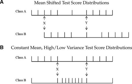
Rank dependent on test score distribution.
Notes: These figures show two classes of eleven students, and each mark represents a student’s test score, increasing from left to right. In (A), the classes have similar score distributions, but the distribution of Class B is shifted higher. This means students with the same absolute scores would have a lower rank in Class B compared to Class A. In (B) the classes have the same mean, minimum, and maximum student test scores, but Class B has a smaller variance. This means students with the same absolute and relative-to-the-class-mean test scores will have different ranks. A student with score Y above the mean will have a higher rank in Class B than Class A, but a student with score X below the mean will have a higher rank in Class A.
However, classes with better resources may be able to generate higher baseline test scores from a given set of students. This is a concern if the impact of such class-level inputs fades differentially to other inputs and if these inputs preserve rank. An extreme example would be if having a good teacher during primary school had a positive impact on baseline test scores, |$Y_{ijsc}^{0}$|, and no impact on secondary outcomes, |$Y_{ijsc}^{1}$|, but being high ability had an impact on both |$Y_{ijsc}^{0}$| and |$Y_{ijsc}^{1}$|. If this were the case, then there would be a problem comparing the test scores of students who were taught by teachers of different effectiveness, because test scores would no longer be a sufficient statistic for all prior inputs.10 Moreover, as any class-level shock would be rank preserving, student rank would become correlated with student ability, even conditional on attainment. The consequence is that transitory, class-level shocks could make class rank a proxy measure for ability, and so confound the estimated rank parameter.
To account for factors that would additively impact all students in a class, such as peers, teachers, or unexpected events on test day, we include fixed effects at the primary class level, denoted by |$\boldsymbol{\mu_{jsc}^{1}}$| in Specifications 1 and 2. These allow for the effects of such class inputs on secondary school outcomes to fade out differentially. In doing so, they account for the mean differences in test scores between Class A and Class B in Panel A. The inclusion of these class effects impacts on the variation that we use for identification. We are now effectively comparing students who have the same test score achievement relative to their class mean during primary school, but different primary ranks due to the test score distribution of their class. We exploit the differences in the test score distributions across schools, cohorts, and subjects.
This follows a similar strategy used by Hoxby (2000), among others, to compare the outcomes of students in adjacent cohorts within the same school. The critical difference is that in these papers, the variation in the treatment is at the school-cohort level (e.g. proportion female), while in our article, there is variation in treatment (rank) within each SSC. Therefore, even though the variation in the test score distribution is at the class level, the variation in the treatment is at the “relative test score by class distribution” level.
As an example, consider a low- and a high-variance class and students at a fixed distance above and below the mean in each class. We have illustrated such a scenario in Panel B of Figure 1. Both classes have the same mean, or have mean differences accounted for via class effects. Here, a student with a test score of Y in Class A would have a lower rank (R = 5) than a student with the same relative test score in Class B (R = 2). In this setting, students above the mean would have a higher rank if they were in the low-variance class compared to if they were in the high-variance class. In contrast, students below the mean would have a lower rank if they were in the low-variance class. So the same change in distribution (from high to low variance) impacts students within the same class differently depending on their relative test scores. That said, this simple illustration only uses variation in the second moment of the test score distribution; in reality, there is considerably more variation at higher moments.11
Note that if the ability distribution of students in a class has an immediate impact on student achievement, this will be captured in the baseline test scores, |$Y_{ijsc}^{0}$|. If the ability distribution of the class impacts the growth in student test scores in that class, then this will be accounted for through the inclusion of class effects, |$\boldsymbol{\mu_{jsc}^{1}}$|.
In our setting, this means we assume that rank is unrelated to potential outcomes conditional on a function of past test scores |$f(Y_{ijsc}^{0})$|, student observables |$\boldsymbol{x_{i}}$|, and SSC attended |$\mu_{jsc}^{1}$| for all ranks. The relation to the thought experiment is that a student’s rank is “as good as” random after conditioning on these factors. There are two types of potential violations. The first type is if |$Y_{ijsc}^{0}$| does not sufficiently capture prior inputs during primary school conditional on primary class fixed effects, |$\boldsymbol{\mu_{jsc}^{1}}$|, which we assume to be additively separable. This would mean that unobserved shocks at |$t=0$| could affect |$Y^{0}$| and |$Y^{1}$| differentially and correlate with rank at the individual-subject level. An example of such a transitory shock would be primary school teachers who teach to specific parts of the achievement distribution and whose impact is only revealed in secondary school outcomes. The second type is if students sort into classes based on what their rank would be. Note, conditioning on |$\boldsymbol{\mu_{jsc}^{1}}$| accounts for any sorting on the basis of class characteristics. Violations of both types are tested for in the robustness analyses in Sections 5.3 and 5.1, respectively.
3. Institutional Setting, Data, and Descriptive Statistics
This section explains the administrative data and institutional setting in England that we use to estimate the rank effect using the specifications of Section 2.1.
3.1. The English school system
The compulsory education system in England is comprised of four key stages. At the end of each stage, students take national exams. Key Stage 2 is taught during primary school, when students are between the ages of 7 and 11. Within each primary school year group, students are further divided into classes of no more than 30 students. English primary schools are typically small, with a median cohort size of 27 students. Coincidentally, the mean class size of a primary school is also 27 students (Falck et al., 2011), so while we do not have data on student class assignment within a primary school-cohort, in the vast majority of cases there will be only one class per school-cohort. We therefore consider a SSC primary rank to be equivalent to the class rank in that subject.12 At the end of the final year of primary school, when the students are age 11, they take tests in English, Maths, and Science. These national tests are externally scored on a scale of 0 to 100, and these results from our baseline measure of achievement.
After completing primary school, students enrol in secondary school and start working towards Key Stage 3. The average primary school sends students to six different secondary schools, while the typical secondary school receives students from 16 different primary schools. Hence, upon arrival at secondary school, the average student has 87% new peers. This large re-mixing of peers allows us to estimate the impact of rank from a previous peer group on subsequent outcomes. If this were not the case and students instead kept their same peers from primary school, our primary rank measure would be correlated with rank in secondary school, and so the rank parameter would also capture the impact of contemporaneous rank.13 Importantly, since 1998, it has been unlawful for schools to select students on the basis of ability; therefore, admission into secondary school does not depend on end-of-primary test scores or student ranking.14 This means that the age-11 exams are low-stakes with respect to secondary school choice. Key Stage 3 takes place over three years; at the end of the final year, at age 14, students take another set of national examinations in the same three subjects. Like the age-11 exams, the age-14 exams are externally scored on a scale of 0 to 100.15
At the end of Key Stage 3, students can choose to take a number of GCSE (General Certificate of Secondary Education) subjects for the Key Stage 4 assessment, which occurs two years later at the age of 16 and marks the end of compulsory education in England. The final grades consist of nine levels (A{*}, A, B, C, D, E, F, G, and U), to which we have assigned points according to the Department for Education’s guidelines (Falck et al., 2011). However, students have some discretion in choosing the number, subject, and level of GCSEs they study. Thus, GCSE grade scores are inferior measures of student achievement compared to age-14 examinations, which are scored on a finer scale and examine all students in the same compulsory subjects. Therefore, we focus on age-14 test scores as the main outcome measure, but also present results for the higher-stakes age-16 examinations.
After Key Stage 4, some students choose to stay in school to study A-Levels for two years, which are a precursor for university-level education. This constitutes a high level of specialization, as students typically only enrol in three A-Level subjects out of a set of 40. For example, a student could choose to study biology, economics, and geography, but not English or maths. Importantly, the A-Level courses they choose will determine the majors they can enrol in during university, which have longer run effects on careers and earnings (Kirkeboen et al., 2016). For example, chemistry as an A-Level is required to apply for medicine degrees and maths is a prerequisite for studying engineering.16 To study the lasting impact of rank, we examine how primary school rank in three subjects affects the likelihood that a student will choose to stay on at school and study those subjects at A-Level.
3.2. Student administrative data
The Department for Education collects data on all students and all schools in the English state education system in the National Pupil Database (NPD).17 The NPD contains data for each individual student, including the schools they attended and their demographic information [gender, Free School Meals Eligibility (FSME), and ethnicity]. It also tracks each student’s attainment data throughout their key stage progression.
Our sample follows the population of five cohorts of students from age 10/11, when they took their Key Stage 2 examinations, through to age 17/18, when they completed their A-Levels. This student sample took their age-11 exams in the academic years 2000–01 to 2004–05; hence, it follows that their age-14 exams took place in 2003–04 to 2007–08, and that the data from completed A-Levels comes from the years 2007–08 to 2011–12.18
We impose a set of restrictions on the data to obtain a balanced panel of students. We use only students who can be tracked with valid age-11 and age-14 exam information and background characteristics. This constitutes 83% of the five cohort population. Next, we exclude students who appear to be double counted (1,060). We also remove students whose school identifiers do not match within a year across datasets, which excludes approximately 0.6% of the remaining sample (12,900). Finally, we remove all students who attended a primary school where the cohort size was less than 10, as these small schools are likely to be atypical in a number of dimensions (e.g. classes formed of students from more than one cohort/year-group). This represents 2.8% of students.19 This leaves us with approximately 454,000 students per cohort, with a final sample of just under 2.3 million students, or 6.8 million student-subject observations.
Descriptive statistics of the main estimation sample
| Mean | SD | Min | Max | |
|---|---|---|---|---|
| Panel A: Student test scores | ||||
| |$\quad$| Age-11 national test scores percentile | ||||
| |$\qquad$| English | 50.285 | 28.027 | 1 | 100 |
| |$\qquad$| Maths | 50.515 | 28.189 | 1 | 100 |
| |$\qquad$| Science | 50.005 | 28.026 | 1 | 100 |
| |$\quad$| Age-11 rank | ||||
| |$\qquad$| English | 0.488 | 0.296 | 0 | 1 |
| |$\qquad$| Maths | 0.491 | 0.296 | 0 | 1 |
| |$\qquad$| Science | 0.485 | 0.295 | 0 | 1 |
| |$\qquad$| Within student rank SD | 0.138 | 0.087 | 0 | 0.577 |
| |$\quad$| Age-14 national test scores percentile | ||||
| |$\qquad$| English | 51.233 | 28.175 | 1 | 100 |
| |$\qquad$| Maths | 52.888 | 27.545 | 1 | 100 |
| |$\qquad$| Science | 52.908 | 27.525 | 1 | 100 |
| |$\quad$| Age-16 national test scores percentile | ||||
| |$\qquad$| English | 41.783 | 26.724 | 1 | 94 |
| |$\qquad$| Maths | 43.074 | 27.014 | 1 | 96 |
| |$\qquad$| Science | 41.807 | 26.855 | 1 | 94 |
| |$\quad$| Age-18 subjects completed | ||||
| |$\qquad$| English | 0.123 | 0.328 | 0 | 1 |
| |$\qquad$| Maths | 0.084 | 0.277 | 0 | 1 |
| |$\qquad$| Science | 0.108 | 0.31 | 0 | 1 |
| Panel B: Student background characteristics | ||||
| |$\quad$| FSME | 0.146 | 0.353 | 0 | 1 |
| |$\quad$| Male | 0.499 | 0.5 | 0 | 1 |
| |$\quad$| Minority | 0.163 | 0.37 | 0 | 1 |
| Panel C: Observations | ||||
| |$\quad$| Students | 2,271,999 | |||
| |$\quad$| Primary schools | 14,500 | |||
| |$\quad$| Secondary schools | 3,800 | |||
Notes: 6,815,997 student-subject observations over 5 cohorts. Cohort 1 takes age-11 examinations in 2001, age-14 examinations in 2004, age-16 examinations in 2006, and A-levels at age 18 in 2008. Test scores are percentalized by cohort-subject and come from externally marked national exams. Age-16 test scores mark the end of compulsory education. Age-18 information could be merged for a sub-sample of 5,147,193 observations from cohorts 2 to 5. For a detailed description of the data, see Section 3.
The key stage test scores at each age group are transformed to have a uniform distribution by subject and cohort. Specifically, test scores are converted into a national test score percentile, so that each individual has nine test scores between zero and 100 (ages 11, 14, and 16). This does not impinge on our estimation strategy, which relies only on variation in test score distributions at the SSC level.20
Table 1 shows descriptive statistics for the estimation sample. Given that the test scores are represented in percentiles, all three subject test scores at age 11, 14, and 16 have a mean of around 50, with a standard deviation of about 28. Recall that the age-11 and age-14 exams are graded out of 100, while the age-16 exam is scored on a much coarser letter-grade scale. This difference explains why the age-16 average percentile scores are lower. Almost 60% of students decide to stay and continue their education until the A-Levels, which are the formal gateway requirement for university admission. Although there are many subjects to choose from, about 14% of students choose to sit an A-Level exam in English, while in maths and science the proportions are about 9% and 11%, respectively.
Information relating to the background characteristics of the students is shown in Panel B of Table 1. Half of the students in the population are male, and more than four-fifths are white British. About 15% are FSME students, which is used as a standard measure of low parental income. The within-student standard deviation across the three subjects (English, maths, and science) is 12.68 national percentile points at age 11, with similar variation in the age-14 tests. This is important, as it shows that there is within-student variation, which is used in student fixed effects regressions.
3.3. Measuring ordinal rank
As explained in Section 3.1, all students take the end-of-primary national exam at age 11. For each subject, we transform the score into national student percentiles by cohort. We use these percentiles to rank students in each subject within their primary school cohort. We take this rank measure as a proxy for perceived ranking based on interactions with peers over the previous six years of primary school, along with repeated teacher feedback. We assume test performance to be highly correlated with everyday classroom performance, and representative of previous performance on any informal class examinations.21
This percentile class rank remains ordinal in nature and still does not carry cardinal information (i.e. information about relative ability distances). For the ease of exposition, we will refer to |$R_{ijsc}$| as the ordinal class rank for the remainder of this article. Panel A of Table 1 shows descriptive statistics of the rank variable.
Now that we have defined our measurement of rank, it is relevant to consider what students will know about their academic rank. While we have complete access to the finely graded test score data, students are instead given only one of five broad attainment levels, with 85% of students achieving one of the top two levels.23 Therefore, neither the students nor their teachers are informed of our ranking metric based on these age-11 test scores. This means our main dependent variable is prone to measurement error due to student perception.
While we cannot know for certain if our measurement of rank based on students’ academic achievement is a good proxy for student perceptions, we have three facts that support this claim. First, a longstanding body of literature from the field of psychology has established that individuals have accurate perceptions of their rank within a group but not of their absolute ability (e.g. Anderson et al., 2006). Second, using merged survey data we find that, conditional on test scores, students with higher ranks in a subject have higher confidence in that subject (Section 7.4.1). And third, if individuals (students, teachers, or parents) had no perception of the rankings, then we would expect not to find an impact of our rank measurement at all. To this extent, the rank coefficient |$\beta_{Rank}^{1}$| from Section 2 will be attenuated, and we are estimating a reduced form of perceived rank using actual rank. In Section 5.3, we also simulate increasingly large measurement errors in the age-11 test scores, which we use to calculate rank, to document what would occur if these tests were less representative of students’ abilities and social interactions. We show that increased measurement error in baseline achievement slightly attenuates the rank estimate, which is consistent with students having a poor perception of their academic rank.
3.4. Survey data: the longitudinal study of young people in England
We have additional information about a sub-sample of students through a representative survey of 16,122 students from the first cohort. The Longitudinal Survey of Young People in England (LSYPE) is managed by the Department for Education and follows a single cohort of teenagers, collecting detailed information on their parental background, academic achievements, and subject confidence.
We merge survey responses with our administrative data using a unique student identifier. Not all students could be matched, as the LSYPE also surveys students attending private schools that are not included in the national datasets, and not all students could be accurately tracked over time. A total of 3,731 survey responses could not be matched. Additionally, 823 state school students did not fully answer the relevant questions and so could not be used in the analysis. This leaves us with 11,558 usable student observations. Even though this does not contain information on each student in a school-cohort, by matching the main data, we can calculate where each LSYPE-student is ranked during primary school.
Students taking the LSYPE survey at age 14 are asked how good they consider themselves in the subjects of English, maths, and science. We code five possible responses in the following way: (2) – Very Good; (1) – Fairly Good; (0) – Don’t Know; (|$-$|1) – Not Very Good; (|$-$|2) – Not Very Good At All. We use this simple scale as a measure of subject-specific confidence (Table 2, Panel A).24 The LSYPE respondents are very similar to students in the main sample, with the mean age-11 scores always being within one national percentile point. That said, the two samples do have differences, with the LSYPE sample having a higher proportion of FSME (18% versus 14.6%) and minority (33.7% versus 16.3%) students. This is to be expected, however, as the LSYPE intended to over sample students from disadvantaged groups.25
LSYPE sample: descriptive statistics
| Mean | SD | Min | Max | |
|---|---|---|---|---|
| Panel A: Student descriptive statistics | ||||
| |$\quad$| How good do you think you are at... | ||||
| |$\qquad$| English | 0.928 | 0.928 | -2 | 2 |
| |$\qquad$| Maths | 0.944 | 0.917 | -2 | 2 |
| |$\qquad$| Science | 0.904 | 1.008 | -2 | 2 |
| |$\quad$| Age-11 national test scores percentile | ||||
| |$\qquad$| English | 50.114 | 27.725 | 1 | 100 |
| |$\qquad$| Maths | 50.783 | 28.378 | 1 | 100 |
| |$\qquad$| Science | 49.453 | 28.287 | 1 | 100 |
| |$\quad$| Age-11 rank | ||||
| |$\qquad$| English | 0.496 | 0.295 | 0 | 1 |
| |$\qquad$| Maths | 0.501 | 0.297 | 0 | 1 |
| |$\qquad$| Science | 0.489 | 0.294 | 0 | 1 |
| |$\qquad$| Within student rank SD | 0.137 | 0.089 | 0 | 0.575 |
| |$\quad$| Student characteristics | ||||
| |$\qquad$| FSME | 0.180 | 0.384 | 0 | 1 |
| |$\qquad$| Male | 0.498 | 0.500 | 0 | 1 |
| |$\qquad$| Minority | 0.337 | 0.473 | 0 | 1 |
| Panel B: parental descriptive statistics | ||||
| |$\quad$| Any post-secondary qualification | 0.323 | 0.468 | 0 | 1 |
| |$\quad$| Gross household income>£33,000 | 0.219 | 0.413 | 0 | 1 |
| |$\quad$| Occupation | ||||
| |$\qquad$| English | 0.014 | 0.119 | 0 | 1 |
| |$\qquad$| Maths | 0.031 | 0.175 | 0 | 1 |
| |$\qquad$| Science | 0.036 | 0.185 | 0 | 1 |
| |$\quad$| Parental time investment in schooling | ||||
| |$\qquad$| Number attending parents evening | 1.213 | 0.713 | 0 | 2 |
| |$\qquad$| Special meeting with teacher about child | 0.235 | 0.424 | 0 | 1 |
| |$\qquad$| Frequency of talking with child’s teacher | 2.124 | 0.957 | 1 | 5 |
| |$\qquad$| Involved in child’s school life | 2.969 | 0.782 | 1 | 4 |
| |$\quad$| Parental financial investment in schooling | ||||
| |$\quad$| Paying for any out of school tuition | 0.234 | 0.423 | 0 | 1 |
| |$\qquad$| English tuition | 0.057 | 0.232 | 0 | 1 |
| |$\qquad$| Maths tuition | 0.027 | 0.163 | 0 | 1 |
| |$\qquad$| Science tuition | 0.019 | 0.137 | 0 | 1 |
| Panel C: Observations | ||||
| |$\quad$| Students | 10,318 | |||
| |$\quad$| Primary schools | 4,137 | |||
| |$\quad$| Secondary schools | 780 | |||
Notes: The LSYPE sample consists of 34,674 observations from the cohort 1 who took age-11 exams in 2001 and age-14 exams in 2004. For a detailed description of the data see Section 3.
The LSYPE also contains detailed parental information (Table 2, Panel B). These characteristics are represented by a set of indicator variables, such as parental qualifications (defined by any parent having post-secondary qualification) and gross household income above £33,000. We use information on parent characteristics to test for sorting to primary schools on the basis of rank conditional on performance in Section 5.1. To test if there is additional sorting to primary schools by subject, we have classified the parental occupation of each parent to each subject. Then, we create an indicator variable for each student-subject pair to capture if they have a parent who works in that field. For example, a child of a librarian and a science technician would have parental occupations coded as English and science, respectively.26
Finally, information regarding parental time and financial investments in schooling is used to explore possible mechanisms in Section 7.2. It is possible that parents may adjust their investments according to student rank during primary school. Therefore, we have coded four forms of self-reported parent time investment: the number of parents attending the most recent parent evening27; whether a parent has arranged a meeting with the teacher; how often a parent talks to the teacher; and how personally involved the parent feels in their child’s school life.28 In our sample, on average, 1.2 parents attended the last parents evening, 23.5% had organized a meeting with the teacher, they have meetings less than once a term, and felt fairly involved in the child’s school life.
4. Main Results
Figure 2 replicates the stylized example from Figure 1 using six primary school English classes from our data. Each class has the same minimum, maximum, and mean (dashed line) test score in the age-11 English exam. Each class also has a student at the 92nd national achievement percentile, but because of the different test score distributions, each of those students has a different rank in their class. This rank is increasing from school one to school six with ranks |$R$| of 0.83, 0.84, 0.89, 0.90, 0.93, and 0.94, respectively, despite all six students having the same absolute and relative-to-the-class-mean test scores. Figure 3 extends this example of the distributional variation by using the data from all primary schools and subjects in our sample. Here, we plot age-11 test scores, de-meaned by primary SSC, against the age-11 class ranks in each subject. The vertical thickness of the plot is the support for the rank distribution. For students close to the median in their class, ranks range from |$R=0.2$| to |$R=0.8$|, showing we have wide support for inference in-sample. This variation exists because classes are small and achievement distributions differ.
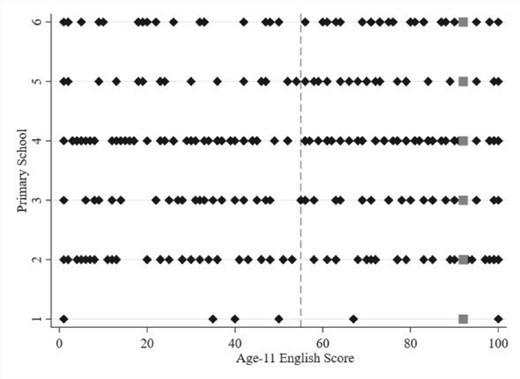
Test score distributions across similar classes
Notes: This graph presents data from six primary school English classes that all have a mean test score of 55 (as indicated by the dashed grey line) and a student scoring the minimum and maximum. Each diamond represents a student score, and grey squares indicate all students who scored 92. Given the different test score distributions, each student scoring 92 has a different rank. This rank is increasing from School 1 to School 6 with ranks of 0.83, 0.84, 0.89, 0.90, 0.925, and 0.94, respectively, despite all students having the same absolute and relative-to-the-class-mean test score. Note that some test scores have been randomly anonymized to protect individuals and schools; this does not affect the interpretation of these figures.
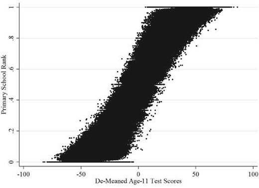
Rank distributions across SSCs
Notes: The Y-axis is the primary rank of students, and the X-axis shows the de-meaned test scores by primary SSC. Note that some test scores have been randomly anonymized to protect individuals and schools; this does not affect the interpretation of these figures.
The main estimates of the impact of primary school rank on secondary school outcomes are presented in Table 3. The first two columns show the impact on age-14 test scores. Column 1 allows for a cubic in prior test scores and primary SSC effects, and column 2 additionally controls for student demographics (ethnicity, gender, ever FSME). The interpretation of the estimate from column 1 is that ranking at the top of class compared to the bottom, ceteris paribus, is associated with a gain of 7.946 national percentiles (0.29 standard deviations). When accounting for student characteristics, there is an insignificant reduction to 7.894, implying that characteristics are not correlated with rank.
This rank parameter is large in comparison with other student characteristics. For example, females score 1.398 national percentiles higher than males, and FSME students on average score 3.107 national percentiles lower than non-FSME students. To gauge the size of this rank effect, we scale it by the standard deviation of rank. A one standard deviation increase in rank is associated with increases in later test scores by 0.084 standard deviations, or 2.35 national percentiles.29
Columns 3 and 4 of Table 3 show an equivalent set of results for the same students two years later, after taking the national exams at the end of compulsory education. The impact of primary school rank on test performance has decreased by a small amount between ages 14 and 16. Comparing columns 2 and 4, being at the top of class compared to the bottom during primary school increases age-16 test scores by 6.389 national percentiles compared with 7.894 at age 14. Here, a one standard deviation increase in primary rank improves later test scores by 1.89 national percentiles.
Rank effects on student outcomes
| Age-14 test scores | Age-16 test scores | Complete subject age-18 | ||||
|---|---|---|---|---|---|---|
| (1) | (2) | (3) | (4) | (5) | (6) | |
| Primary rank | 7.946*** | 7.894*** | 6.468*** | 6.389*** | 0.025*** | 0.025*** |
| 0.147 | 0.147 | 0.154 | 0.152 | 0.002 | 0.002 | |
| Male | -1.398*** | -2.526*** | -0.012*** | |||
| 0.045 | 0.056 | 0.000 | ||||
| FSME | -3.107*** | -4.329*** | -0.017*** | |||
| 0.030 | 0.041 | 0.000 | ||||
| Minority | 1.978*** | 4.329*** | 0.045*** | |||
| 0.054 | 0.083 | 0.001 | ||||
| Cubic in age 11 test scores | |$\surd$| | |$\surd$| | |$\surd$| | |$\surd$| | |$\surd$| | |$\surd$| |
| Primary SSC effects | |$\surd$| | |$\surd$| | |$\surd$| | |$\surd$| | |$\surd$| | |$\surd$| |
Notes: Results obtained from six separate regressions based on 2,271,999 student observations and 6,815,997 student-subject observations. In columns 1 and 2, the dependent variable is by-cohort-by-subject percentalized KS3 test scores. In columns 3 and 4, the dependent variable is by-cohort-by-subject percentalized KS4 test scores. In columns 5 and 6, the dependent variable is an indicator for completing an A-Level at age 18 in the corresponding subject. SSC effects are fixed effects for each primary school-by-subject-by-cohort combination. Standard errors in italics and clustered at the secondary school level (3,800). Significance levels *** 1%,** 5%, * 10%.
After the examinations at age 16, students can choose to study for A-Levels, the qualifications required to study at university. We estimate the impact of primary school rank in a specific subject on the likelihood of choosing to study that same subject for A-Levels.30 These results are presented in columns 5 and 6 of Table 3, with the binary outcome variable being whether or not the student completed an A-Level related to that subject. In this linear probability model, conditional on prior test scores, student characteristics, and SSC effects, students ranked at the top of the class in a subject compared to the bottom are 2.5 percentage points more likely to choose that subject as an A-Level. Assuming a linear relationship, a one standard deviation increase in rank increases the likelihood of choosing that subject by 0.74 percentage points. As one in ten students complete these subjects at A-Level, a one standard deviation increase in class rank during primary school represents a 7% increase in the probability of choosing the associated A-Level seven years later.
5. Robustness
This section examines the robustness of our main results in four dimensions. First, we test the conditional independence assumption by testing if student characteristics are correlated with rank, conditional on test scores and SSC effects. Second, we test if the estimates are robust to alternate functional forms of prior achievement. Third, we examine if systematic or non-systematic measurement error in the age-11 achievement test scores would result in spurious rank effects. Finally, we address miscellaneous concerns such as school sizes, classroom variance, and the proportion of new peers at secondary school.
5.1. Rank-based primary school sorting
Our first key assumption (A1) is that a student’s rank in a subject is effectively random conditional on achievement and primary school-cohort attended. This would not be the case if parents were selecting primary schools based on the rank that their child would have. However, parents typically want to get their child into the best school possible in terms of average grades (Rothstein, 2006; Gibbons et al., 2013). This would work against any positive sorting by rank, the parents most motivated to do this would be enrolling their child in the schools with higher attainment, and so the child would have a lower rank. Regardless, in order for parents to sort on the basis of rank, they would have to know the ability of their child and of all their child’s potential peers by subject, which is unlikely to be the case when parents are making this choice when their child is only four years old.31
Appendix Section A.1 details two sets of tests which provide evidence against sorting. First, we use the LSYPE sample to show that pre-determined parental characteristics that impact future achievement, such as occupation, qualifications, or income, are uncorrelated with student rank conditional on age-11 test scores and SSC effects. This implies that parents are not selecting primary schools on the basis of rank. Second, we use the main sample to test whether pre-determined student characteristics are correlated with student rank, conditional on age-11 test scores and SSC effects. There are small correlations between student rank and characteristics; however, the coefficients are inconsistent and small. For example, using the largest treatment change possible, students ranked at the top of the class compared to the bottom are 0.8% more likely to be female and 0.8% more likely identify as a minority. To assess the cumulative effect of these small imbalances, we test whether predicted age-14 test scores are correlated with primary rank. We obtain the predicted test scores by re-estimating the main specification without the rank parameter and using the resulting parameters. We find that primary rank does have a small positive relationship with predicted test scores, albeit only about 1/70th of the magnitude of our main coefficient. A one standard deviation increase in rank increases predicted test scores by 0.001 standard deviations. These results are consistent with the fact that our main estimates in Table 3 hardly change when including student characteristics.32
In summary, it appears that parents are not choosing schools on the basis of rank, but there are small imbalances in predetermined student characteristics. These imbalances could be caused by students with certain characteristics having rank concerns during primary school (Tincani, 2015), and who therefore exert just enough effort to gain a higher rank. We return to this subject when discussing specifications that include individual effects that would absorb student competitiveness (Section 5.4) and having competitiveness as a potential mechanism (Section 7). Regardless of the sources of these imbalances, they do not significantly affect our results, as they are precisely estimated to be extremely small.
5.2. Specification checks
Recall that our second main assumption (A2) is that we have not misspecified the main equation such that it generates a spurious result. To test this, Appendix Table A.4 shows rank estimates from six specifications with increasing higher order polynomials for prior test scores. We find that once there is a cubic relationship, the introduction of additional polynomials makes no significant difference to the parameter estimate of interest. The final column replaces these polynomials with an indicator variable for each national test score percentile. With this flexible way of conditioning on prior achievement, we again see no meaningful change in the rank parameter, with an estimate of 7.543 (0.146).
Specification 1 also requires that the test score parameters be constant across schools, subjects, and cohorts, after allowing for mean shifts in outcomes through the inclusion of SSC effects. In Appendix Table A.5, we relax this requirement and allow the impact of the baseline test scores to be different by school, subject, or cohort by interacting the polynomials with the different sets of fixed effects. We again find that allowing the slope of prior test scores to vary by these groups does not significantly impact our estimates of the rank effect.33
5.3. Test scores as a measure of ability
To ensure that rank is conditionally orthogonal to potential outcomes, we account for student characteristics, SSC effects, and age-11 test scores. The intention is to have conditional test scores as an accurate measure of the underlying ability of the student. The inclusion of SSC effects accounts for any factor that impacts the growth of test scores between age 11 and age 14 at the class level. However, there may be other factors that occur during primary school that could cause these test scores to be a poor measure of ability. These sources of measurement error are a concern if they are rank preserving, as it would mean that the rank parameter could pick up the underlying student ability rather than the impact of rank itself. In the following, we outline situations where test scores do not reflect the underlying student ability due to systematic measurement error and the general case of non-systematic measurement error (noise).
5.3.1. Systematic measurement error
We consider two types of systematic measurement error in test scores that would be rank preserving. The first type is measurement error that impacts the level of measured student attainment. Such error could be generated from primary school peer effects. The second type is measurement error that impacts the spread of measured student achievement, which could be generated by primary school teachers. In either case, if these factors caused a permanent change in student ability, they would be fully accounted for by conditioning on the end-of-primary-school test scores.
The concern is that if these factors cause measurement error in observed ability, but preserve rank, then rank could pick up mismeasured ability. Appendix Section A.2 discusses the issue of primary school peer effects in more detail and provides tests to establish that the inclusion of SSC effects accounts for a range of inflated peer effects. Appendix Section A.3 sets out how teacher effects could generate a spurious correlation through increasing the spread of test scores.34 We provide three distinct tests that demonstrate teacher scaling effects are not driving the results. In doing so, we also establish that we do not need to rely on second central moment differences in classroom ability distributions to estimate the rank effect.
5.3.2. Non-systematic measurement error
When students take a test, their scores will not be a perfect representation of how well they perform academically on a day-to-day basis; they instead provide a noisy measure of ability. This type of non-systematic measurement error is potentially problematic for our estimation strategy, as it could generate a spurious relationship between student rank and gains in test scores. This is because they are both subject to the same measurement error but to different extents.
The intuition for this bias is as follows: when measurement errors are relatively large, they will impact both test scores and rank measures. Individuals with a mistakenly high (or low) test score also have a falsely high (or low) rank. Then, as we are estimating the growth in test scores, these students would have lower (higher) observed growth, which would downward bias the rank parameter. At low levels of measurement error, rankings would not change and it would be possible for the rank measure to pick up some information about ability that is lost in the test score measure.
Consider the simplest of situations where there is only one group and two explanatory variables, individual |$i's$| ability |$X_{i}^{*}$|, and class ability ranking |$R_{i}^{*}$|. Assume |$X_{i}^{*}$| cannot be measured directly, so we use a test score |$X_{i}$| as a baseline, which is a noisy measure of true ability and has measurement error |$X_{i}=l_{i}(X_{i}{}^{*},e_{i})$|. We also use this observed test score |$X_{i}$| in combination with the test scores of all others in that group |$X_{-i}$| to generate the rank of an individual, |$R_{i}=k(X_{i},X_{-i})$|. We know this rank measure is going to be measured with error |$e_{i2}$|, such that |$R_{i}=h_{i}(R_{i}^{*},e_{i2})$|. The problem is that this error, |$e_{i2}$|, is a function of their ability |$X_{i}^{*}$| and their own measurement error |$e_{i}$|, but also depends on the ability and measurement errors of all other individuals in their group (|$X_{-i}^{*}$| and |$e_{-i}$|, respectively): |$R_{i}=k(l_{i}(X_{i}^{*},e_{i}),l_{-i}(X_{-i}^{*},e_{-i}))=f(X_{i}^{*},e_{i},X_{-i}^{*},e_{-i}). $| Therefore, any particular realization of |$e_{i}$| not only causes noise in measuring |$X_{i}^{*}$|, but also in |$R_{i}^{*}$|. This means we have correlated, non-linear, and non-additive measurement error, where |$COV(e_{i},e_{i2})\ne0$|. This specific type of non-classical measurement error is not a standard situation, and it is unclear how this would impact the estimated rank parameter.35
We gauge the importance of this problem by performing a data-driven bounding exercise. This involves a set of Monte Carlo simulations where we add additional measurement error drawn from a normal distribution (|$\mu=0$|) to the test score measure of each student, then recalculate student ranks and re-estimate the specification at ever-increasing variances of measurement error. In doing so, we are informed of the direction and the approximate magnitude of any measurement error-induced bias. The variance of this distribution increases from 1% of the standard deviation in test scores up to 30%. In terms of test scores, this represents an increase in the standard deviation from 0.28 to 11.2. For each measurement error distribution, we simulate the data 1000 times and estimate the rank parameter.
Figure 4 shows the simulated estimates of the mean and the 2.5th and 97.5th percentiles from the sampling distribution of beta for each measurement error level. We see that as measurement error increases, there is a slight downward bias. Consistent with our stated intuition, this bias grows non-linearly with measurement error. Small additional measurement error has little impact on the results. The amount of downward bias from increasing the additional error from 1% to 20% of a standard deviation amounts to the same level of bias as increasing the error from 20% to 25%.
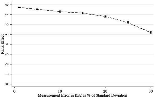
Estimates from Monte Carlo simulations with additional measurement error in baseline test scores
Notes: This figure plots the mean rank estimate from 1000 simulations of Specification 1 with increasing additional measurement error added to student baseline test scores 7 with increasing additional measurement error added to student baseline test scores before computing ranks. The measurement error is drawn from a normal distribution with mean zero and a standard deviation that is proportional to the standard deviation in baseline test scores (28.08). The measurement error of each subject within a student is independently drawn. The error bars represent the 2.5th and the 97.5th percentiles from the sampling distribution of beta for each measurement error level.
Appendix Figure A.1 repeats this process with alternative types of measurement errors. Panel A presents mean estimates from a heterogeneous measurement error process, where the impact of the normally distributed error increases as the test score is farther away from the national mean. This is reflective of the examinations potentially being less precise at extreme values. This slightly exacerbates the downward bias and the non-linearity of the bias. Next, Panel B draws the additional measurement error from the uniform distribution, which results in smaller downward bias. Given that these national tests have been designed to measure ability in a subject and additive measurement error causes only a small downward bias, we conclude that our main estimates are attenuated, at most, very little.
Finally, we show that multiplicative measurement error (rather than additive measurement error) also does not bias our results. Specifically, we consider measurement error that increases as students’ ability is further from the average. This result is dependent on the achievement distribution being uniformly distributed. With a normally distributed achievement distribution, there can be large measurement error in the tails of the distribution without changes in ranks (real or observed). As a result, the rank parameter picks up some measure of ability that has been masked by the measurement error. One way this can be undone is to transform the observed ability distribution into a uniform distribution. This means that the measurement error in observed test scores always has the same impact on student rank (in expectation), regardless of where they are in the observed ability distribution. This removes the spurious rank effect. We present data-generating processes confirming this result in Appendix Section A.4. As we use the uniformly distributed national student percentiles to rank students, we are immune from this source of bias.
5.4. Further robustness checks: within-student estimates, class size, re-mixing of students, and prior peers
To address potential remaining concerns, we present four further robustness checks. First, we have seen some student demographics predict rank conditional on prior test scores. Despite their apparent economically insignificant size, they may reflect larger unobservable differences between high- and low-ranked students. To address such concerns, we exploit the fact that we have measures for student achievement across three subjects. This allows us to estimate the main specification with the addition of student fixed effects, |$\tau_{i}^{1}$|, which is a component of the error term in Specification 1. This will account for any student-level unobservable characteristic or shock that impacts growth between age-11 and age-14 test scores, such as competitiveness, parental investment, or school investments. Note that this will also absorb any general growth in achievement across all subjects due to student rank, which should be considered part of the rank effect. This estimate is providing a lower bound on the rank effect, because it is only representing the additional gains in a subject due to the prior rank in that same subject in primary school. One could interpret it as the extent of subject specialization due to primary school rank.
Alternative specifications: age-14 test scores
| Main effect | Effect within student | ||
|---|---|---|---|
| (1) | (2) | ||
| (1) | Main specifications - benchmark | 7.894*** | 4.562** |
| 0.147 | 0.107 | ||
| (2) | Small primary schools (single class) only | 6.469*** | 3.646*** |
| 0.176 | 0.146 | ||
| (3) | Randomized school within cohort | -0.099 | -0.227 |
| 0.130 | 0.150 | ||
| (4) | No prior peers in secondary school | 10.461** | 5.011*** |
| 0.449 | 0.415 | ||
| (5) | Excluding specialist secondary schools | 7.875*** | 4.586*** |
| 0.155 | 0.112 | ||
| (6) | Accounting for secondary-cohort subject FX | 7.942*** | 4.471*** |
| 0.146 | 0.106 | ||
| Student characteristics | |$\surd$| | Abs | |
| Cubic in age 11 test scores | |$\surd$| | |$\surd$| | |
| Primary SSC effects | |$\surd$| | |$\surd$| | |
| Student effects | |$\surd$| | ||
Notes: This table is discussed in Section 5 (rows 1–4) and in Section 7.2 (rows 5 and 6). Results obtained from 12 separate regressions. Rows 1, 2, 3, 4, 6 and 9 use the main sample of 6,815,997 student-subject observations. Row 5 uses a reduced sample of 2,041,902 student-subject observations who attended primary schools with cohort sizes of less than 31. Row 7 is estimated using a sample of 452,088 student-subject observations from students who had no primary peers in secondary school. Row 8 uses a reduced sample of 6,235,806 student-subject observations from students who did not attend a secondary school classified as specialist. The dependent variable is by-cohort-by-subject percentilised KS3 test scores. Student characteristics are ethnicity, gender, and Free School Meal Eligibility (FSME). SSC effects are fixed effects for each school-by-subject-by-cohort combination. The second column presents corresponding estimates for rank effects within student only. Standard errors in italics and clustered at the secondary school level. Significance levels *** 1%,** 5%, * 10%.
Table 4 contains two columns of estimates. The first column presents rank estimates from the indicated specifications. The second column presents the same estimates including student effects. This column is a series of tests to determine if student-level unobservables are driving the effect, which would be evidenced by the effect becoming insignificant. As expected, the within-student estimates in column 2 are considerably smaller. The first row of Table 4 shows the estimate from the main specification on age-14 test scores is 7.894. When accounting for student-level unobservables, including general rank effects, this falls to 4.562. In terms of effect size, the within-student standard deviation of the national percentile rank is 11.32, the standard deviation of the rank within student is 0.138, and therefore a one standard deviation increase in rank increases test scores by 0.056 standard deviations.36 Despite the reduction, the within-student estimate continues to be statistically significant when the main estimate is significant.
Second, we have been describing our estimates as the impact of academic standing within one’s primary school class. This is because we rank students within their SSC, and the median cohort size of primary schools is 27. Given that the legal maximum class size for 11 years old students is 30, we argue that primary SSCs are effectively equivalent to classes. However, some schools have larger cohorts and so our rank measure would represent their position within their SSC rather than their classroom. Row 2 of Table 4 presents estimates that restrict the sample to only those students who attended a primary school of less than 31 students per cohort. Here, the estimate falls slightly to 6.469 and the standard errors increase due to a smaller sample, but the rank effect remains.
Third, one might be concerned that there is an mechanical relationship between rank and later achievement due to the way rank is measuring underlying ability. To address this, row 3 of Table 4shows estimates from the main specification, but using data where we have randomly allocated students to primary schools within a cohort and recalculated their ranks. Here, students are very unlikely to be assigned to a class with their actual peers. As expected, this generates precise zero effects, reflecting that rank metrics do not innately predict future outcomes, but are setting dependent.
The fourth and final robustness check that we perform relates to the re-mixing of peers when students leave primary school and enter into secondary school. We claim we are estimating the impact of primary school rank, but if rank in primary school and secondary school are correlated, then we may be estimating the cumulative impact of rank. For example, a student having exactly the same peer group in primary and secondary school would likely have the same rank in both settings, and so the primary school rank parameter would reflect the impact of rank in primary and secondary school on age-14 outcomes.
To test this, we calculate the correlation between primary and secondary ranks based on primary school test scores, conditional on test scores, SSC, and student demographics. On the subsample of students who have no old peers (451,000), there is an extremely low correlation between primary and secondary ranks of 0.02.37 Using this same subsample, we find that the rank effect does not decrease (Table 4, Row 7), implying that the main estimates are not driven by a continuation of the rank treatment, but rather the rank in primary school.38
6. Heterogeneity of the Impact of Rank
6.1. Impact by subject
Our main specification stacks student achievement across subjects and assumes a constant impact across subjects. Panel A of Table 5 shows the estimates of the rank parameter separately for English, science, and maths (e.g. the impact of a student’s rank in English at age 11 on their test scores at age 14). We can see that the impact is similar across subjects, ranging from 7.400 for English up to 8.820 for maths.39
Subject-specific educational production
| Age-14 test scores | |||
|---|---|---|---|
| English (1) | Science (2) | Maths (3) | |
| Panel A: same subject effects | |||
| |$\quad$| Rank | 7.400*** | 8.373*** | 8.820*** |
| 0.202 | 0.192 | 0.188 | |
| Panel B: cross subject effects | |||
| |$\quad$| English rank | 5.423*** | 1.417*** | -0.140 |
| 0.189 | 0.163 | 0.138 | |
| |$\quad$| Science rank | 0.597*** | 5.566*** | 3.233*** |
| 0.171 | 0.167 | 0.137 | |
| |$\quad$| Maths rank | 0.788*** | 3.612*** | 7.753*** |
| 0.178 | 0.174 | 0.173 | |
| Student characteristics | |$\surd$| | |$\surd$| | |$\surd$| |
| Cubic in age-11 test scores | |$\surd$| | |$\surd$| | |$\surd$| |
| Primary SSC effects | |$\surd$| | |$\surd$| | |$\surd$| |
Notes: Each column of Panel A estimates Specification 1 separately by subject. Each column of Panel B additionally allows for cross-subject effects of ranks and test scores. Standard errors in italics and clustered at the secondary school level (3,800 schools). Significance levels ***1%,**5%, *10%.
The main specification also does not allow for spillovers between subjects. The lower half of Table 5 allows for these effects. Each column in Panel B represents a single student-subject level estimation, where we condition on the rank and prior test scores in each subject separately. The impacts of rank on the same-subject outcomes are on the main diagonal, and the impacts of rank on outcomes in other subjects are off the diagonal. For each subject, once we allow for the impact of rank from another subject, the main coefficient reduces in size. One explanation for this could be that ranks are positively correlated across subjects, and there are positive spillovers across subjects. We also see that the nature of the spillover effects depends on the subject pairing. Science and maths ranks have a negligible impact on English test scores (0.597 and 0.788, respectively); on the other hand, the impacts of maths rank on science test scores and science rank on maths scores are considerably larger at 3.612 and 3.233, respectively.40
6.2. Non-linearities and heterogeneity
6.2.1. Age-14 outcomes
We replace the single linear rank parameter |$\beta_{Rank}^{1}$| with the impact of rank at each ventile of primary rank (|$\lambda=1,...,20$|) plus two indicators for the highest- and lowest-ranked students. The reference group is the tenth ventile, comprised of those in the middle of the rank distribution (Specification 2). Figure 5.1 shows these rank estimates for the impact on age-14 test scores without and with and without student fixed effects. The effect of rank appears to be linear throughout the rank distribution, with small flicks in the tails. Students ranked just above the median perform better three years later than those at the median. The within-student estimates are smaller in magnitude throughout and have a smaller gain for being top of the class.
Continuing to use this non-linear specification without student fixed effects, we estimate the heterogeneity by gender and Free School Meal Eligibility by interacting the rank variables with these two characteristics. Figure 5 shows how rank relates to the gains in later test scores by gender. Males are more positively affected by having an above-median rank, gaining almost twice as much from being at the top of class. In contrast, males are less effected by rank in the bottom half of the distribution, meaning that females are marginally more negatively affected by having a low rank compared to males.41
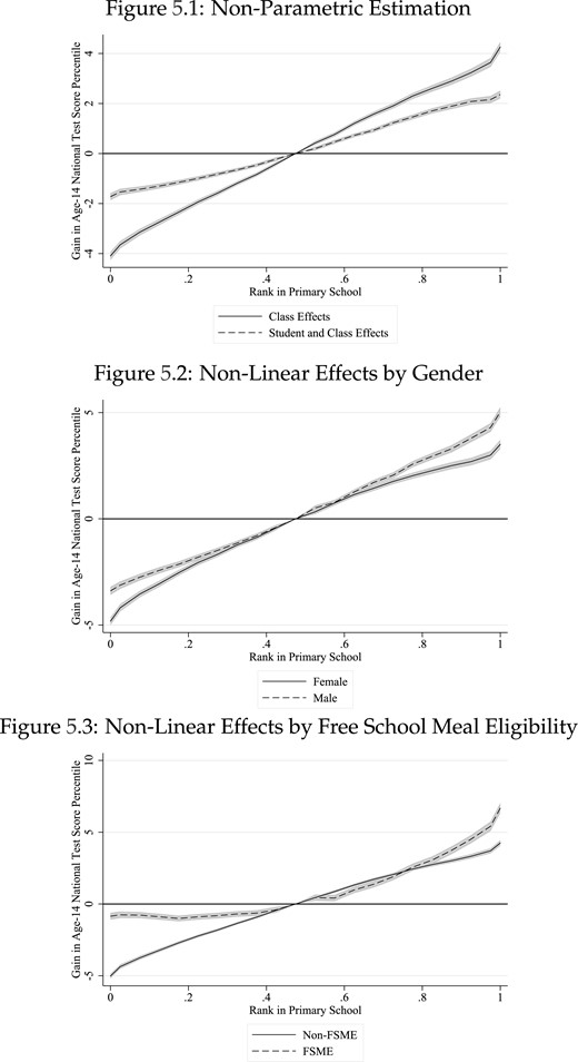
Impact of primary rank on age-14 test scores
Notes: The figures show the impact of rank in primary school using versions of Specification 2, allowing the effect of rank to vary by ventile and including a dummy for being top or bottom of class (SSC). The reference ventile is composed of those students from the 45–50th percentiles. Effects obtained from estimating the effect of rank on non-FSME (female) students and the interaction term with FSME (male) students. All estimates have cubic controls for baseline test scores and condition on SSC effects and student effects. Shaded area represents 95% confidence intervals. Standard errors are clustered at the secondary school level.
That males gain more from being high-ranked and lose less from being low-ranked could be due to differential perception of rank by gender. It is entirely possible that males perceive themselves to be higher-ranked than they actually are. In this reduced form specification, we cannot separate the impact of actually being highly ranked from the perception of higher rank, and heterogeneity could result from either.
Finally, Figure 5 shows the relationship between rank and future test scores by FSME status. Both types of students show a positive relationship between rank and later test scores; however, FSME students are less negatively affected by a low rank and more positively affected by a high rank. The relationship is approximately flat for FSME students in the bottom half of the rank distribution but becomes much steeper in the top half of the distribution. In fact, we find that FSME students gain almost twice as much as non-FSME students from having the highest rank in a class.
One possible explanation for this is that FSME students may lack confidence in their abilities and thus the idea of being low-ranked is not as disconcerting to them. On the other hand, the shallower gradient for non-FSME students in the top half of the rank distribution suggests that they are less positively affected by higher class rank, but more negatively affected by lower rank. These students’ academic confidence may be influenced more by factors outside of school. We will return to the interpretation of these effects at the end of the mechanisms section.
6.2.2. A-level subject choices
Figure 6 presents the non-linear impacts of primary school rank on A-Level subject choices. The three panels in this figure present the impact of rank in each subject on the likelihood of choosing an English, maths, or science A-Level. In each panel, we see a positive relationship between the rank in the subject in question and taking that A-Level at the end of secondary school. Unlike the impact on test scores, these impacts are non-linear with the majority of the impacts occurring in the top decile. There are differences across subjects. For maths, students are just as likely to choose this subject at A-Level if they were at the bottom of their primary class as in the middle; it is only the students at the very top for whom rank has an effect. For both English and science, students are always more likely to choose those subjects as primary rank increases.
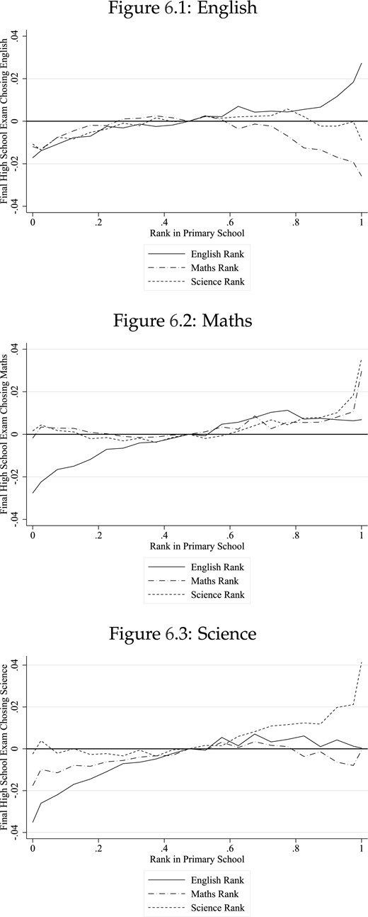
Impact of primary subject-rank on A-level choices
Notes: The figures show the impact of rank in each of the three subjects in primary school on the likelihood of completing each of the subjects at the A-Level. The estimates come from a version of Specification 2, allowing the effects of rank to vary by ventile. The reference ventile is composed of those students from the 45–50th percentiles. Each panel represents the results from three separate regressions for each subject rank (and baseline test scores) in primary school. The take-up rates for the A-level subjects are English 12.3%, maths 8.4%, and science 10.8%.
Figure 6 also plots spillover effects across subject. Being low-ranked in English reduces the chances of students choosing any A-Level subject. Students are also less likely to take A-Level English if they are highly ranked in either science or maths. This type of negative spillover across subjects does not occur with test scores. An explanation for this is that students are limited to taking only three A-Levels in total, therefore having a high rank in one subject might crowd out other subjects.
7. Mechanisms
A number of different mechanisms related to the rank of the student may produce these results, including competitiveness, parental investment, environmental favourability to certain ranks, students learning about their ability, and development of non-cognitive skills. In the following section, we discuss how each of these channels might explain the findings presented in the previous sections.
7.1. Mechanism 1: competitiveness
Recent research indicates that students may have rank concerns during primary school and that they adjust their effort accordingly (see Tincani, 2015; Hopkins and Kornienko, 2004; Kuziemko et al., 2014). In our setting, if students work harder during primary school because of these concerns, it will be reflected in higher end-of-primary school achievement scores, which we control for. However, if students want to maximize rank at minimal cost of effort, this potentially could produce the slight imbalances found in Section 5.1 but not negative effects of low ranks. One could consider this as a form of measurement error in ability, but one that is caused by the rank of the student.
To illustrate this point, consider students attending primary schools where they face little competition for being at the top of the class. These students could spend less effort and get by with lower test scores while still remaining at the top of the class. Then, when facing a more competitive secondary school environment, these previously “coasting” students may exert more effort and will appear to have high growth in test scores. This would generate a positive rank effect, as those at the top of class have high gains in test scores. Extending this thought experiment to the rest of the class, lower-ranked students would be consistently exerting effort in primary and secondary school and so would not generate this type of rank effect. Therefore, if this type of rank concern is driving the results, we would only see these effects near the top of the rank distribution. However, we find that there is an impact of rank throughout the rank distribution (Figure 5); as such, we do not believe competition for top of class is driving the results..42
7.2. Mechanism 2: parental investment
Parents may react to the academic rank of their child by altering their investment decisions. For instance, parents may assist the child at home with homework or extra-curricular activities, or choose a school that specializes in a certain subject. If the parents know that their child is ranked highly in one subject, they may have a tendency to encourage the child to do more activities and be more specialized in that subject. If parental investment focused on the weaker subject (Kinsler et al., 2014), this would reverse the rank effect for these students
We use information from the LSYPE survey to show that while parental investments during secondary school are correlated with a student’s rank during primary school, this is only true when not conditioning on achievement. The same is true for secondary school choice. We take this as direct evidence against rank-based parental investments as a cause of the positive long-run effects of primary rank during secondary school. More generally, parents of children in the English school system are unlikely to be accurately informed of their child’s specific class rank. Teacher feedback to parents will convey some information, such as the student being the best or worst in class, but it is doubtful that they would be able to discern a difference from being near the middle of the cohort rankings. Our results, however, show significantly different effects from the median for all ventiles with SSC effects. Taken together, parental investments are an unlikely mechanism.
To test for increased parental investment by subject, we categorize information from the LSYPE survey on parental investments during secondary school in terms of time and money. Panel A of Table 6 shows the relationship rank has with parental time investments during secondary school. The first column shows the correlation with rank without conditioning on student achievement. The second column shows estimates from our main specification (1). Rank in primary school is positively correlated with time investments, but once we condition on primary school achievement, there is no longer a significant relationship. This is true of all the measures of time investment and of the index of these measures.43 Panel B of Table 6 shows how parental financial investments during secondary school are related to primary rank. Again we find that investments are correlated with student rank, until we condition on prior achievement.
Parental investments and secondary schools
| (1) | (2) | |
|---|---|---|
| Panel A: parental time investments | ||
| |$\quad$| Number of parents attending parents evening | 0.248*** | -0.167 |
| 0.033 | 0.102 | |
| |$\quad$| Special meeting with teacher about child | -0.119*** | 0.053 |
| 0.018 | 0.062 | |
| |$\quad$| Frequency of talking with child’s teacher | -0.215*** | 0.170 |
| 0.041 | 0.129 | |
| |$\quad$| Involved in child’s school life | 0.028 | -0.114 |
| 0.034 | 0.110 | |
| |$\quad$| Index of parental school involvement | -0.224*** | 0.042 |
| 0.086 | 0.146 | |
| Panel B: parental financial investments | ||
| |$\quad$| Paying for any out of school tuition | 0.148*** | -0.066 |
| 0.018 | 0.062 | |
| |$\quad$| Paying for out of school tuition by subject | -0.029*** | -0.007 |
| 0.006 | 0.026 | |
| Panel C: sorting to secondary by subject value added | ||
| |$\quad$| Unconditional value added | |$\it 0.365^{***}$| | -0.002 |
| 0.016 | 0.009 | |
| |$\quad$| Conditional value added | |$\it 0.367^{***}$| | -0.002 |
| 0.016 | 0.010 | |
| |$\quad$| Cubic in age 11 test scores (excluding panel A) | |$\surd$| | |
| |$\quad$| Primary SSC effects | |$\surd$| | |$\surd$| |
Notes: Results obtained from 18 separate regressions. Regressions in Panels A and B are based on 11,558 student observations and 34,674 student-subject observations from the LSYPE sample. For descriptives, see Table 2. Regressions from Panel C use the main sample. Secondary school subject specific value added is calculated in terms of age-11 to 14 growth in test score percentiles recovered from a secondary school subject fixed effect. These fixed effects have been standardised to mean zero and standard deviation one. Cohort effects are not included because the LSYPE data is only available for one cohort. Standard errors in parentheses and clustered at the secondary school level (796/3800), Significance levels *** 1%,** 5%, * 10%.
In the final panel of Table 6, we test for sorting to secondary schools by subject according to primary rank rather than additional parental investment. Our goal here is to answer the question, “Do parents send their children to schools with higher value-added measures in the subjects they are ranked highly in?” We calculate each secondary school’s subject-specific, value-added measure in terms of growth in test score percentiles from age 11 to age 14. The first row uses a raw value-added measure, and the second uses one that conditions on student demographics; each has been standardized to mean zero and standard deviation one. Both measures provide similar results: students ranking high in a subject tend to enrol in schools with a high value-added measure in that subject. Like the previous panels, though, when we account for age-11 achievement, there is no significant relationship.44
Instead of testing for sorting directly, the final two rows of Table 4 explore how the main rank coefficient changes when we condition on secondary school characteristics. As secondary school characteristics can be interpreted as possible outcomes of primary rank in their own right, these parameters should be interpreted with caution. We proceed by first removing from the sample all students who attend secondary schools specializing in English, maths, or science.45 Excluding these students has a negligible impact on the rank effects (Row 5, Table 4). Second, we consider that parents may not be reacting to labels but are instead choosing schools because of the school’s high actual gains in certain subjects. If the rank effect is due to this type of parental sorting, then conditioning on secondary SSC effects would reduce the size of the rank parameter. In Row 6 of Table 4, we show that these additional controls only have a small impact on the rank effect, as would be expected given the results from Panel C of Table 6.
7.3. Mechanism 3: rank-based investments
Another possible explanation for the positive impact of rank is that there are rank-based investments by schools. For example, one can imagine primary school teachers focusing additional attention on low-ranked students or schools providing such students with extra resources. These investments would not impact our results if they had a permanent impact on student achievement, as they would be captured in end-of-primary-school test scores. This mechanism requires that any improvement in test scores be transitory; that is, the improvement is realized in either primary school or secondary school, but not both. Like the competitive mechanism, one can consider this as a form of rank-generated measurement error.
For example, if teachers provide additional attention to low-ranked students, these students would achieve higher age-11 test scores than otherwise, but their low ranking would be preserved. These students would also have low achievement growth between ages 11 and 14, which would generate a positive rank correlation at the bottom of the distribution.46 For positive rank correlation to occur at the top of the distribution would require the opposite, that is, increased investment in top students during primary school would not be reflected in primary school test scores but only in later achievement. This would be captured by our rank effect, |$\beta_{Rank}^{1}$|, and would be considered a potential mechanism.
Both of these channels require the targeting of teacher effort. However, in our setting teachers work within a performance-related pay system, where principals and teachers agree on a target achievement level for each individual student, and teachers are then rewarded for generating better-than-average improvements in performance (Atkinson et al., 2009). Much like the pay-for-percentile system discussed by Barlevy and Neal, (2012), this pay system offers no additional financial incentive for teachers to target low-performing or low-ranked students. Moreover, Chakrabarti, (2014) and Reback et al., (2014) have demonstrated that teachers fail to target specific groups of students even when offered explicit incentive schemes. Ultimately, as awards are based on student growth, primary schools teachers are incentivized to generate gains in contemporaneous test scores rather than gains that will only be realized in secondary school. Between these incongruencies and the required assumption that any beneficial effects be transitory, we feel rank-based investment is unlikely to be the dominant mechanism behind the rank effect.
7.4. Mechanism 4: student confidence
A simple mechanism to explain the rank effect is that being highly ranked among peers makes an individual more confident in school either generally or in a specific subject. We first provide evidence that rank, conditional on test scores, increases confidence, and the heterogeneity of these results mirrors that found with the test score outcomes. To explain the positive effects of primary rank on confidence and attainment, we then propose and test two models of student effort based on learning and non-cognitive skills.
7.4.1. Impact on confidence
The LSYPE sample responded to questions regarding student confidence in each of the subjects of interest at the age of 14. This allows us to test directly if rank position within primary school has a lasting effect on subject confidence. The specification for this test is equivalent to Specification (1) with the dependent variable now being subject-specific confidence. Since this survey was run for only one cohort, the SSC effects are replaced with school-by-subject effects.
The first column of Table 7 presents our main result using only the students from the LSYPE sample. We obtain a rank effect of 8.977, a slight but not statistically significant increase over our baseline estimates. The second column shows that students with a higher primary school rank are significantly more likely to say that they are good in that subject. Moving from the bottom of the class to the top increases a student’s confidence by 0.196 points (0.2 standard deviations) on a five-point scale. A one standard deviation increase in student rank increases later confidence by 5.8% of a standard deviation. This suggests that students develop a lasting sense of their strengths and weaknesses based on their local rank position, conditional on relative test scores.47 Columns 3 and 4 present results separately for boys and girls. In line with our results from the administrative data, we find that boys’ confidence is more strongly affected by primary rank.
Overall, given the effects of rank on the direct measures of student confidence and the heterogeneity of effects found in the main results, it seems likely that confidence matters.48 This is in line with the psychological literature, which finds that academic confidence is thought to be especially malleable at the primary school age (Tidemann, 2000; Leflot et al., 2010; Rubie-Davies, 2012).
Student confidence on rank
| Age-14 | Subject | Male—subject | Female—subject | |
|---|---|---|---|---|
| test scores | confidence | confidence | confidence | |
| (1) | (2) | (3) | (4) | |
| Primary rank | 8.977*** | 0.196** | 0.285* | -0.009 |
| 1.602 | 0.093 | 0.168 | 0.210 | |
| Male | -1.939*** | 0.124*** | ||
| 0.259 | 0.014 | |||
| FSME | -2.588*** | 0.046** | 0.032 | 0.026 |
| 0.383 | 0.019 | 0.037 | 0.038 | |
| Minority | 2.107*** | 0.159*** | 0.113*** | 0.219*** |
| 0.414 | 0.022 | 0.038 | 0.045 | |
| Cubic in age-11 test scores | |$\surd$| | |$\surd$| | |$\surd$| | |$\surd$| |
| Primary SSC effects | |$\surd$| | |$\surd$| | |$\surd$| | |$\surd$| |
Notes: Results obtained from four separate regressions based on 11,558 student observations and 34,674 student-subject observations from the LSYPE sample (17,415 female, 17,259 male). For descriptives, see Table 2. The dependent variable is a coarse measure of confidence by subject. Cohort effects are not included because the LSYPE data is only available for one cohort. Standard errors in parentheses and clustered at the secondary school level (796). Significance levels ***1%,**5%, *10%.
7.4.2. Learning or non-cognitive skills?
Increased confidence could improve student test scores via two channels: learning about ability and non-cognitive skills.
The first channel entails students using their ordinal class ranking in addition to their absolute achievement to learn about their own subject-specific abilities, similar to a model proposed by Ertac, (2006). Students then use this information when deciding how to allocate effort by subject in secondary school. Critically, we assume that this mechanism does not change an individual’s education production function, only their perception of it. We will argue below that this feature allows us to test the learning model.
The second channel supposes that a student’s ordinal ranking during primary school has an impact on their academic confidence and hence non-cognitive skills. In the educational literature, this effect is known as the Big-Fish-Little-Pond Effect, and it has been found to occur in many different countries and institutional settings (see Marsh et al., (2008) for a review).49 This confidence can differ between subjects, so a student could, for example, consider herself good in English, but bad in maths (Marsh et al., 1988; Yeung and Lee, 1999). Confidence generates non-cognitive skills in a subject such as grit, resilience, and perseverance Valentine et al., (2004).50 We assume that these increased non-cognitive skills reduce the student’s cost of effort for that task.51
Students maximize total grades subject to a cost function. This cost function is determined by their cost of effort in each subject |$C_{is}$| and a general cost of academic effort |$C_{ig}$|. This general cost reflects a student’s attitude towards education in general and is linear in the sum of effort applied across all subjects, |$E_{im}+E_{ie}$|. The total cost of effort |$T$| that a student can apply is fixed; however, the inclusion of a general cost of academic effort term means that the total effort applied by a student is very flexible.
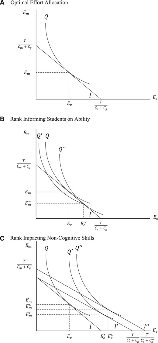
Optimal allocation of effort across subjects, confidence model
Notes: These figures show students’ optimal effort allocation between maths (|$E_{m}$|) and English (|$E_{e}$|). Students have costs of effort for each subject, |$C_{m}$| and |$C_{e}$|, and a general cost of effort, |$C_{g}$|. Students are willing to provide a total cost of effort |$T$|, have perceived iso-quants |$Q$| and iso-costs |$I$|. In (B), under the learning-about-abilities model, |$Q^{\sim}$|represents perceived iso-quant, where |$E_{e}^{\sim}$| and |$E_{m}^{\sim}$| are the resulting chosen effort levels in English and maths, respectively. In (C), under the non-cognitive skills model, |$Q'$| and |$I'$| represent the iso-quant and iso-cost lines with lower costs of English effort, where |$E_{e}^{'}$| and |$E_{m}^{'}$| are the resultant chosen effort levels. Finally, |$Q''$| and |$I''$| represent the iso-quant and iso-costs with lower costs of English effort and lower costs of general academic effort, where |$E''_{e}$| and |$E''_{m}$| are the resultant chosen effort levels. For more details, see Section 7.4.2.
In the learning-about-ability model, students know their costs of effort but do not know their abilities. Therefore, in the experience phase, students use their test scores and relative ranking to form beliefs about their abilities, which determines the shape of their isoquant. Students experiencing a high rank in English in the primary period believe that they have a high ability |$A_{e}^{\sim}$| in that subject. They therefore optimize according to the new isoquant |$Q^{\sim}$|and devote more effort to English in the secondary period (|$E_{e}^{\sim}$|) because they believe this will generate high marginal returns to effort (Figure 7, Panel B).
In the non-cognitive skills model, students know about their costs of effort and their abilities in each subject. Here, in the experience phase, students develop confidence in the subjects in which they are ranked highly and develop positive non-cognitive skills in that subject, which we model as reducing the cost of effort |$C_{e}>C_{e}^{'}$|. This shifts the students’ iso-cost line out along the |$E_{e}$|-axis to point |$T/(C_{e}^{'}+C_{g})$|. Consequently, they are able to reach higher isoquant |$Q^{'}$|, and optimally invest more effort in English, |$E_{e}^{'}>E_{e}$| (Figure 7, Panel C). Rank can also impact students’ general cost of effort |$C_{g}$|, which we assume to be a decreasing function of ranks in all subjects. If there are any general gains in confidence due to having a high rank in English, they will reduce the cost of any academic effort |$C_{g}>C_{g}^{'}$| and cause a parallel shift out of the iso-cost line, with intercepts |$T/(C_{m}+C_{g}^{'})$| and |$T/(C_{e}^{'}+C_{g}^{'})$|. This results in the students providing more effort to all subjects |$E_{e}^{''}>E_{e}^{'}>E_{e}$|. Note that with this channel, it will be impossible for students to misallocate effort across subjects, as they are perfectly informed about their costs and abilities.
Given these two ways of interpreting confidence, we now consider the case where students have a high rank locally, in their class, but a low rank globally. Under the learning hypothesis, students with large differences between local and national ranks would have more distorted information about their true abilities, assuming national test scores are a good measure of ability. These students would then be more likely to misallocate effort across subjects, thereby achieving lower average grades compared to students whose local ranks happen to closely align with national ranks. Turning back to Panel B of Figure 7, this is represented by the student believing that she is on iso-quant |$Q^{\sim}$| with resulting effort choices |$E_{e}^{\sim}$|and |$E_{m}^{\sim}$|, which are not optimal because her perceptions are incorrect. Such a student would therefore over-invest effort in English. The local rank provides a distortion that shifts effort allocation from the optimal allocation (|$E_{e}$| and |$E_{m}$|) to a non-optimal allocation (|$E_{e}^{\sim}$| and |$E_{m}^{\sim}$|). This means that due to the misinformation about relative abilities, students ultimately end up on a lower iso-quant than they could achieve |$Q^{'}<Q$|.
This gives rise to a testable hypothesis to distinguish between the learning and non-cognitive skills channels. In situations where local ranks are very different from national ranks, and thus less informative about actual abilities, the misinformation can result in students obtaining lower total grades. Conversely, if the rank effects are caused by actual changes in the costs associated with the education production function, even if local rank were different from national rank, this would not lead to a misallocation of effort in terms of maximising grades, and so total grades would not decrease. To summarize, if a student experiences a local rank in English higher than their national rank, under both models they allocate more effort into English in the second period, but under the non-cognitive skills hypothesis this would not lead to a misallocation of effort and lower average grades.
Here, |$\bar{Y}_{ijc}^{1}$| denotes the average test scores across subjects in period |$1$|, |$\bar{R}_{ijc}$| is average rank in primary school, |$\bar{M}$| the additional misinformation variable, |$\boldsymbol{x_{i}}$| is a vector of individual characteristics, and |$\boldsymbol{\varphi_{jc}^{1}}$| represents primary school-cohort fixed effects. To clearly restate our hypothesis: if the amount of misinformation causes students to misallocate effort across subjects, we expect |$\beta_{M}^{1}<0$|. Alternatively, the null hypothesis that local rank causes changes to the actual production function means |$\beta_{M}=0$|.
For benchmarking purposes, we first estimate a version of Specification (8) without the additional misinformation variable (Table 8, Column 1). The effect of average rank on average test score is estimated at 10.765, and is statistically significant at the 1% level. Column 2 adds the coefficient for the effect of misinformation. The misinformation coefficient is slightly positive but statistically insignificant at conventional levels while the rank parameter remains almost unchanged. We repeat this in columns 3 and 4 controlling for student characteristics and find no meaningful differences. Given these results, we fail to reject the null hypothesis that the degree of misinformation does not cause students to misallocate effort. Therefore, we conclude that the learning mechanism alone is unlikely to generate our results.
With this in mind, we turn back to reinterpret the main results. The non-cognitive skills model is consistent with the empirical results found in Section 4. We can then interpret the smaller estimates from the individual fixed effects specifications as being due to the absorption of any general confidence effects, |$C_{g}$| (or |$I^{''}$| to |$I^{'}$| in Figure 7). These within-student estimates only capture the change in effort allocation due to changes in the relative costs of effort across subjects.
Is the degree of misinformation harmful?
| Age-14 test scores | ||||
|---|---|---|---|---|
| (1) | (2) | (3) | (4) | |
| Primary rank | 10.765*** | 10.768*** | 10.678*** | 10.672*** |
| 0.226 | 0.225 | 0.225 | 0.224 | |
| Misinformation | 0.103 | -0.172 | ||
| 0.266 | 0.264 | |||
| Student characteristics | |$\surd$| | |$\surd$| | ||
| Cubic in age-11 test scores | |$\surd$| | |$\surd$| | |$\surd$| | |$\surd$| |
| Primary-cohort effects | |$\surd$| | |$\surd$| | |$\surd$| | |$\surd$| |
Notes: Results obtained from four separate regressions based on 2,271,999 student observations averaged over subjects where columns 2 and 4 include an additional explanatory variable of the degree of misinformation. The dependent variable is age-14 test scores. Rank is the average rank across English, maths, and science in primary school. The misinformation measurement is the average absolute difference between local rank and national percentile rank for each student in the end-of-primary school test score as explained in Section 7.4.2. Student characteristics are ethnicity, gender, and Free School Meal Eligibility (FSME). Standard errors in italics and clustered at 3,800 secondary schools. Significance levels *** 1%,** 5%, * 10%.
8. Conclusion
We establish that an individual’s ordinal position within a group impacts later objective outcomes, controlling for cardinal achievement. In doing so, we have introduced a new factor in the education production function. Rank position within primary school has significant effects on secondary school achievement and the likelihood of completing STEM subjects. There is significant heterogeneity in the effect of rank, with males being influenced considerably more. Moreover, a higher rank is linked to important non-cognitive skills, such as confidence.
These findings lead to a natural question for parents deciding where to send their child: Should my child attend a “prestigious school” where she will have a lower rank, or a “worse school” where she will have a higher rank? Rank is just one of the many factors in the education production function, so choosing solely on the basis of rank is unlikely to be a prudent approach.
To gauge the relative importance of rank for choosing a primary school, we follow an approach similar to Chetty et al., (2011) to estimate the aggregate effect of all class inputs (class size, teacher quality, peer quality, etc.) on long-run outcomes, using the size of our SSC effects from Specification 1 as a benchmark. Attending a primary school with a one standard deviation higher impact is associated with a 0.269 standard deviation increase in age-14 test scores. In contrast, a one standard deviation increase in rank increases age-14 test scores by 0.084 standard deviations. Therefore, the impact of rank is about 30% of the size of lasting class effects.
We now make some comparisons with effect sizes found by the literature. We first compare the rank effect to the impact of teachers for one academic year. Being taught by a teacher who is one standard deviation better than average for one academic year improves student test scores by 0.1 to 0.2 standard deviations (Rivkin et al., 2005; Aaronson et al., 2007). Comparatively, we find that having a one standard deviation higher rank throughout six years of primary school increases age-14 achievement by 0.08 standard deviations. Note however, that these teacher effects on test scores are contemporaneous and fade out over time (Chetty et al., 2014), whereas the rank effect is long-lasting.
There are few papers that look directly at the long-run impact of elementary school peers on later outcomes, with one notable exception being Carrell et al., (2018). They estimate that the presence of a single disruptive peer in a class of 25 throughout elementary school has the causal effect of reducing test scores in Grades 9 and 10 by 0.02 standard deviations. In comparison, we estimate the long-run effect of a one standard deviation increase in rank throughout primary school to be equivalent in magnitude to the addition of four disruptive peers.
Our results also show that primary school rankings affect A-Level subject choices and thus have long-run implications, as A-Level choices are linked directly to university admissions.53 If males and females, on average, had the same primary rankings across all subjects, these findings would not contribute to the STEM gender gap. However, females outrank males in English subjects during primary school, so females have on average higher ranks in non-STEM subjects.54 Taking absolute differences in combined maths and science versus English ranks, males have a 0.166 higher rank in STEM subjects than females. This difference means that males are 0.66 percentage points more likely choose a STEM subject as an A-Level. Given the low share of students taking STEM subjects, if we were to equalize the primary rankings in subjects across genders, this would reduce the total STEM gender gap by about 7%. One direct way to achieve this would be to separate primary schools by gender, ensuring an equal number of females and males at the top of their class for all subjects.
The existence of heterogeneity in the rank effects means that there are potential gains to be made from re-grouping students across classes. To illustrate this point, consider two types of students: Type A that is highly impacted by rank, and Type B that is not impacted. Assume both have abilities drawn from the same uniform distribution. As in our setting, each class contains a small number of students, which results in varying test score distributions across classes. Thus, some classes will have higher average attainment than others.
In this example, swapping an average-ability Type A student in a class with high mean test scores with an average-ability Type B student in a class with low mean test scores would improve net grades. The Type A student would increase in rank, which would improve their test scores. The Type B student would have a lower rank, but their test scores would be unaffected by this. Note that the other students would be unaffected because this swapping of students of the same ability preserves the rank and ability distributions of both classrooms. This is different from the linear-in-means peer effects model, where gains for one student would be offset by losses of other students.
These results may also have implications for what information should be shared. To improve productivity, it would be optimal for managers or teachers to highlight an individual’s local rank position if that individual has a high local rank. If an individual is in a high-performing peer group (where they may have a low local rank but high global rank), a manager should make the global rank more salient. For individuals who have low local and global ranks, managers should focus on absolute attainment or on other tasks where the individual has higher ranks.
Our findings also help to reconcile a puzzle in education research. These persistent rank effects could explain why some achievement gaps increase over the education cycle, such as widening education gaps by race (Fryer and Levitt, 2006; Hanushek and Rivkin, 2006; 2009). With rank effects, small differences in early attainment could negatively affect confidence, leading to decreased investment in education that would exacerbate any initial differences. A similar argument could be made for the persistence of relative age effects, in which older children consistently fare better than their younger counterparts (Black et al., 2011).
Finally, research on selective schools and school integration has shown mixed results from students attending selective or predominantly non-minority schools (Angrist and Lang, 2004; Cullen et al., 2006; Kling et al., 2007; Clark, 2010; Dobbie and Fryer, 2014). Many of these papers use a regression discontinuity design to compare the outcomes of the students that just passed the entrance exam to those that just failed; a majority, though, find that no benefit is derived from attending selective schools.55 However, our findings would speak to why the potential benefits of these schools may be attenuated through the reduction in confidence these students experience upon being placed in a higher-achieving peer group where they have a lower rank. This is consistent with Cullen et al., (2006, p. 1194), who find that those whose peers improve the most gain the least: “Lottery winners have substantially lower class ranks throughout high school as a result of attending schools with higher achieving peers, and are more likely to drop out.”
The editor in charge of this paper was Jerome Adda.
Acknowledgments
We thank Esteban Aucejo, Thomas Breda, David Card, Andrew Clark, Jeff Denning, Susan Dynarski, Ben Faber, Mike Geruso, Eric Hanushek, Brian Jacob, Pat Kline, Steve Machin, Magne Mogstad, Imran Rasul, Jesse Rothstein, Olmo Silva, Kenneth Wolpin, Gill Wyness, and participants of the CEP Labour Market Workshop, UC Berkeley Labor Seminar, the Sussex University, Queen Mary University, and Royal Holloway-University departmental seminars, the CMPO seminar group, the RES Annual Conference panel, IWAEE, the Trondheim Educational Governance conference, the SOLE conference, CEP annual conference, the UCL PhD seminar, the BeNA Berlin seminar, IFS seminar, and the CEE Education Group for valuable feedback and comments. Earlier working paper versions of this article are Murphy and Weinhardt, (2013) and Murphy and Weinhardt, (2014). Weinhardt gratefully acknowledges ESRC seed funding (ES/J003867/1) as well as support from the German Science Foundation through CRC TRR 190 (project number 280092119). All remaining errors are our own.
Supplementary Data
Supplementary data are available at Review of Economic Studies online.
Footnotes
We also address the broader issue of non-systematic measurement error in the baseline test scores. Under certain conditions with non-standard multiplicative measurement error, normally distributed achievement measures would generate a spurious correlation. This is addressed by transforming the outcome measure into percentiles, which we explain in Section 5.3. We also show that non-systematic additive measurement error in achievement would result in a downward bias, which we quantify.
Hoxby and Weingarth, (2005) introduce the invidious comparison peer effect, where being surrounded by better peers also has negative effects.
When students move from primary to secondary school in England, they experience on average 87% new peers. This ensures that our estimate of the effects of primary rank is not confounded by effects of peers, teachers, or rank during secondary school. As a robustness check, we estimate the effects on students with 100% new peers in secondary school and continue to find the impact of primary rank (see Table 4).
Bandiera et al., (2015) find that the provision of feedback improves subsequent test scores for college students. Specifically relating to relative feedback measures, Azmat and Iriberri, (2010) and Azmat et al., (2019) find that their introduction during high school increases productivity in the short run. In contrast, this article does not examine the contemporaneous reaction to a new piece of information but rather examines student reactions to previous ranking.
We show in Section 2.1 that contemporaneous rank effects at primary school are controlled for in our setting, and if these were transitory would lead to a downward bias in the long-run estimate. Cicala et al., (2018) show that status concerns in peer groups can affect students contemporaneous behavioural and academic outcomes.
A nascent and growing literature applies the empirical method set out by this article to estimate contemporaneous (Elsner and Isphording, 2017) and long-run rank effects in education (Denning et al., 2018).
Note these class effects will also account for differential fade out of class-level inputs. This is discussed in more detail in Section 2.2.
The treatment occurs at the primary SSC level, and therefore a strong argument can be made for this being the correct level at which to cluster the standard errors. However, we chose to cluster the standard errors at the secondary school level for two reasons. The first is that all of the outcomes occur during the secondary school phase, where students from different primary schools will be mixing and will be attending the same secondary school for all subjects. Therefore, we thought it appropriate to partially account for this in the error term. Secondly, clustering at the secondary school level rather than the primary SSC is considerably more conservative, generating standard errors that are 50 percent larger. Standard errors are available upon request for other levels of clustering, including primary, primary SSC, and secondary SSC, as well as two-way clustering at the student and SSC level for both primary and secondary schools.
In the robustness section, we show that a rank effect remains after its inclusion to address concerns of shocks occurring at the individual level (e.g. sorting to primary school or parental investment).
This would not be a problem if we make the strong assumption that test scores are a sufficient statistic for all prior inputs. This would mean that all inputs fade at the same rate, or that they do not fade at all, |$\mu_{jsc}^{0}=\mu_{jsc}^{1}$|, only in this case controlling for primary school test scores would be sufficient (Todd and Wolpin, 2003).
In Robustness Section 5.4, we show that the results are largely unaffected by restricting the sample to schools where the maximum number of students per cohort is 30, which is the maximum age-11 class size in England.
In Robustness Section 5.4, we show that the results are unaffected by restricting the sample to students where they have no primary peers. Here, correlation between primary and secondary rank, conditional on age-11 test scores, is extremely low at 0.02.
The Schools Standards and Framework Act 1998 made it unlawful for any school to adopt selection by ability as a means of allocating places. A subset of 164 schools (5%) were permitted to continue to use selection by ability. These grammar schools administer their own admission tests which are independent of KS2 examinations, and admissions are also not based on student ranking within school.
There is no skipping or repeating of grades in the English education system.
For the full overview of subjects that can be chosen, see: http://www.cife.org.uk/choosing-the-right-a-level-subjects.html
The state sector constitutes 93% of the student population in England.
The analysis was limited to five cohorts, as from year 2008–09 on the external age-14 examinations were replaced with teacher assessments.
Estimations using the whole sample are very similar, only varying at the second decimal point.
In addition to ensuring comparability across cohorts, using the national achievement percentile means that any non-systematic measurement error in test scores will not be correlated with the density of students in the achievement distribution. This is important because if such a correlation existed, then it could generate a spurious correlation between rank and test scores. This is discussed further in Section 5.3. We preclude this by using achievement percentiles, which have a uniform distribution.
In English primary schools, it is common for students to be seated at tables of four and for tables to be grouped by pupil ability. Students would be sat at the ‘top table’ or the ‘bottom table’. This would make class ranking, where they rank more salient e.g. “I’m on top table, but I’m the worst; therefore I’m fourth best.”
Other ways of breaking ties produce very similar results. Ranks are computed only for students in our estimation sample.
Using a regression discontinuity design across these achievement levels, with the underlying national score as the running variable, we find no gains for those students who just achieved a higher level. This reaffirms that this is a low-stakes test for the students.
Using more flexible functional forms, such as a dummy for each confidence level, provides evidence that there is an approximately linear relationship between confidence and test scores.
Appendix Table A.5 presents the raw differences and their associated standard errors.
We use the “Parental Standard Occupational Classification 2000” to group occupations into Science, Maths, English, and Other in the following way: Science (3.6%): 2.1 Science and technology, 2.2 Health Professionals, 2.3.2 Scientific researchers, 3.1 Science and Engineering Technicians. Maths (3.2%): 2.4.2 Business And Statistical Professionals, 3.5.3 Business And Finance Associate Professionals. English (1.4%): 2.4.5.1 Librarians, 3.4.1 Artistic and Literary Occupations, 3.4.3 Media Associate Professionals. Other: Remaining responses.
A bi-annual, after-school meeting of students’ parents or guardians to meet with their teachers.
The frequency of meetings with teacher is coded: (1) – Never; (2) – Less than once a term; (3) – At least once a term; (4) – Every 2–3 weeks; (5) – At least once a week. The self-reported parental involvement is coded: (1) – Not Involved At All; (2) – Not Very Involved; (3) – Fairly Involved; (4) – Very Involved.
Another way to gauge the relative importance of rank compared to traditionally important factors is to examine changes in the mean squared error. In a specification with only prior test scores and SSC effects, including a gender term reduces the mean square error by 0.25, an ethnicity term reduces it by 0.28, and the introduction of the rank parameter reduces the mean squared error by 0.31.
Students that did not take on any of the core subjects or have left school are included in the estimations.
Parents could infer the likely distributions of peer ability if there is auto-correlation in student achievement within a primary school. This means that if parents know the ability of their children by subject, as well as the achievement distributions of primary schools, they could potentially select a school on this basis.
Using the methods proposed by Oster, (2017) and conservative assumptions–namely, that it is possible to achieve an |$R^{2}$| equal to one and unobservables are equal to observables in their effect–we cannot generate coefficient bounds that include zero for our main effect.
It would be feasible to estimate the impact of rank within a single group if we assume a smooth relationship between prior and future test scores. The discrete nature of ordinal ranks would generate non-linear jumps in outcomes for marginal increases in baseline achievement. One can consider this to be analogous to a regression discontinuity approach with primary school test scores as the running variable and rank as treatment status, where rank jumps up by one unit whenever the test score exceeds that of the next student in that group. However, this approach would require that students (or whomever is generating the rank effect) know their rank with certainty. This is unlikely to hold in this setting, as in the limit, two students may interpret they have the same rank. Our approach instead only requires that students have an indication of their rank, and classifies students with the same test score as having the same rank. Alternate methods to break ties produce quantitatively similar results.
Note that teacher effects that only cause changes in the level of class achievement are accounted for with the SSC effects, similar to linear-in-means peer effects.
The standard solution to non-classical measurement error is to obtain repeated measurements or instrumental variables (Schennach, 2016). In our case, we do not have another measure of exactly the same test. An alternative would be to use the test scores from another subject as an instrument for |$X_{i}$|. However, as we go on to show in Section 6.1, other-subject ranks do not meet the exclusion restriction, as they have spillover effects across subjects.
For students with similar ranks across subjects, the choice of specialization could be less clear. Indeed, in a sample of the bottom quartile of students in terms of rank differences, the estimated rank effect is 25% smaller than those from the top quartile. Detailed results available on request.
In the full sample, there is a conditional correlation of 0.232. However, some of this is mechanical, as despite students having an average of 87% new peers in secondary school, 13% of peers will be from their primary school, thus primary and secondary ranks cannot be not fully independent.
This also addresses any concerns one may have regarding reflection issues, e.g. one student having a high rank implies another must have a lower rank. Here, we are estimating the impact of rank on students in a setting with entirely new peers. As both the SSC and student effects estimates are larger in size than the benchmark, it implies that any reflection issues would be downward biasing on our estimates.
That the effects are comparable is important for the student fixed effects specifications, which restrict these to be identical.
In Section 5.3, we dealt with concerns regarding measurement error in student test scores. One potential solution would be to instrument test scores in one subject with those from other subjects. The results from Table 5 show that all but one of the subject pairs do not meet the exogeneity criteria. The exception is English rank not impacting maths outcomes. Instrumenting maths rank and test scores with English rank and test scores, we obtain a two-stage least squares estimate of maths rank on maths outcomes of 8.07. This is not significantly different from the main estimate of 7.753 at conventional levels of statistical significance. This again implies that any measurement error in test scores would only cause a small downward bias.
Appendix Figure A.2 shows the equivalent results with a specification that includes individual effects. These effects will absorb any spillover effects across subjects, and so reflect individual specialization. In this setting, males are more affected by rank throughout the rank distribution. Males still gain more from being at the top of the class, but also lose out marginally more from being in the bottom half. These results suggest that males place more importance on relative rank in determining their self-concept than females.
Alternatively, if there were unobserved heterogeneity in competitiveness, this could cause primary school subject rank to be positively correlated with later test scores. However, in the specification that includes student fixed effects, any general competitiveness of an individual is accounted for.
This index is created by principal component analysis of the time investments and standardised to mean zero standard deviation one.
Appendix Table A.6 additionally tests for school level value added, with and without student controls. None of the eight specifications find a significant relationship with rank conditional on prior attainment.
This consists of 8% of all secondary schools at the age of entry, or 575,000 observations in our sample.
Note, if primary teachers taught to the median student in such a transitory way, those at both extremes would lose out. So instead of a linear effect, we would find a U-shaped curve with both students at the bottom and the top of the distribution gaining relatively more during secondary school.
This is despite there being very few LSYPE respondents per primary school (4.5 students, conditional on at least one student being in the survey), which severely limits the degrees of freedom in each primary school subject group.
Note, it is feasible that these effects on confidence are generated through improvement in student performance due to primary rank. As we do not have a measure of student confidence immediately upon leaving primary school, we cannot tell apart the direction of these effects.
The psychological-education literature uses the term “self-concept,” which is formed through our interactions with the environment and peers O’Mara et al., (2006). Individuals can have positive or negative self-concept about different aspects of themselves, and students with a high self-concept would also develop positive non-cognitive skills.
The importance of such non-cognitive skills for both academic attainment and non-academic attainment is now well established (Heckman and Rubinstein, 2001; Borghans et al., 2008; Lindqvist and Vestman, 2011).
The alternative is to have non-cognitive skills impact the ability (returns to effort), by subject, which leads to the same predictions and testable hypothesis.
These comparisons can be in terms of cardinal and ordinal performance.
Hastings et al., (2013) use data from Chile to estimate that choosing STEM subjects at university over humanities increases later earnings by 12%.
The average primary rank for males (females) is 0.440 (0.535) in English, 0.515 (0.468) in maths, and 0.477 (0.474) in science.
Similar effects are found in the higher education literature with respect to affirmative action policies (Arcidiacono et al., 2012; Robles and Krishna, 2012).
Parents could infer the likely distributions of peer ability if there is auto-correlation in student achievement within a primary school. This means that if parents know the ability of their children by subject, as well as the achievement distributions of primary schools, they could potentially select a school on this basis.
Using the methods proposed by Oster, (2017) and conservative assumptions (namely it is possible to achieve an |$R^{2}$| equal to one and unobservables are one-to-one proportional in their effect to observables, we cannot generate coefficient bounds that include zero for our main effect. This includes scenarios where unobservables explain over 125 times more of our remaining unexplained variation compared to student demographics.
References
APPENDIX
A.1. Rank-based sorting to primary school
A core tenet of this article is that a student’s rank in a subject is effectively random conditional on achievement. This would not be the case if parents were selecting primary schools based on the rank that their child would have. To do this parents would need to know the ability of their child and of all their potential peers by subject, which is unlikely to be the case when parents are making this choice when their child is only four years old.56 Moreover, typically parents want to get their child into the best school possible in terms of average grades (Rothstein, 2006; Gibbons et al., 2013), which would work against any positive sorting by rank. We provide two pieces of evidence to test for sorting: by parental characteristics and by student characteristics.
We are most concerned with parental investments that would vary across subjects, because such investments would not be fully accounted for with the student fixed effects specification. One such parental characteristic that could impact investments by subject is the occupation of the parent. Children of scientists may have both a higher initial achievement and a higher growth in science throughout their academic career due to parental investment or inherited ability. The same could be said about children of journalists in English classes and children of accountants in maths classes. This does not bias our results as long as, conditional on age-11 test scores, parental occupation is orthogonal to primary school rank. However, if these parents sort their children to schools such that they will be the top of class and also generate higher than average growth, then this would be problematic.
Differences in characteristics between main and LSYPE samples
| Main sample | LSYPE sample | Difference | Standard error | |
|---|---|---|---|---|
| Panel A: student test scores | ||||
| |$\quad$| Age-11 national test scores percentile | ||||
| |$\qquad$| English | 50.285 | 50.114 | -0.171 | 0.277 |
| |$\qquad$| Maths | 50.515 | 50.783 | 0.268 | 0.278 |
| |$\qquad$| Science | 50.005 | 49.453 | -0.552 | 0.277 |
| |$\quad$| Age-11 rank | ||||
| |$\qquad$| English | 0.488 | 0.496 | 0.008 | 0.003 |
| |$\qquad$| Maths | 0.491 | 0.501 | 0.010 | 0.003 |
| |$\qquad$| Science | 0.485 | 0.489 | 0.004 | 0.003 |
| |$\quad$| Age-14 national test scores percentile | ||||
| |$\qquad$| English | 51.233 | 51.376 | 0.143 | 0.278 |
| |$\qquad$| Maths | 52.888 | 53.779 | 0.891 | 0.272 |
| |$\qquad$| Science | 52.908 | 53.051 | 0.143 | 0.272 |
| Panel B: student background characteristics | ||||
| |$\quad$| FSME | 0.146 | 0.180 | 0.034 | 0.002 |
| |$\quad$| Male | 0.499 | 0.498 | -0.001 | 0.003 |
| |$\quad$| Minority | 0.163 | 0.337 | 0.174 | 0.002 |
| Panel C: Observations | ||||
| |$\quad$| Students | 2,271,999 | |||
| |$\quad$| Primary schools | 14,500 | |||
| |$\quad$| Secondary schools | 3,800 | |||
Notes: The table presents mean characteristics from the main and the LSYPE samples, and their raw differences. The standard errors are unclustered.
Balancing table
| Main effect | Effect within student | |
|---|---|---|
| (1) | (2) | |
| Panel A: parental occupation | ||
| |$\quad$| Age-11 test scores | 8.943*** | 1.534* |
| 1.207 | 0.846 | |
| Panel B: balancing by rank | ||
| |$\quad$| Parental occupation | 0.004 | 0.001 |
| 0.004 | 0.004 | |
| |$\quad$| Parental education | -0.004 | – |
| 0.063 | ||
| |$\quad$| Household income |$>$| £33k | -0.014 | – |
| 0.052 | ||
| |$\quad$| Male | -0.008** | – |
| 0.004 | ||
| |$\quad$| FSME | -0.008*** | – |
| 0.003 | ||
| |$\quad$| Minority | 0.008*** | – |
| 0.002 | ||
| |$\quad$| Predicted age-14 test scores | 0.113*** | – |
| 0.031 | ||
| |$\quad$| Cubic in age-11 test scores (excl. Panel A) | |$\surd$| | |$\surd$| |
| |$\quad$| Primary SSC effects | |$\surd$| | |$\surd$| |
| |$\quad$| Student effects | |$\surd$| | |
Notes: Rows 1 and 2 are based on 31,050 subject-student observations for which parental occupations could be identified from the LSYPE (for details see Section 3.4). Panel A establishes the relevance of the parental occupation variable by estimating effects on age-11 test scores. Panel B shows balancing of rank with the listed student characteristics as dependent variables. Predicted age-14 test scores are generated from a linear projection of student observables and SSC effects. Primary SSC effects are fixed effects for each school-by-subject-by-cohort combination. As parental occupation varies across subjects within a student, regressions in column 2 include additional student fixed effects. Standard errors in italics and clustered at the secondary school level (3,800). Significance levels *** 1%,** 5%, * 10%.
Simulation of rank estimation with peer effects
| Mean peer effects | Non-linear peer effects | |||
|---|---|---|---|---|
| (1) | (2) | (3) | (4) | |
| Panel A: Rank has no effect |$\beta_{rank}= 0.0$| | ||||
| Mean |$\hat{\beta}_{rank}$| | 0.046 | 0.000 | 0.302 | -0.041 |
| Mean SE of |$\hat{\beta}_{rank}$| | 0.014 | 0.018 | 0.015 | 0.019 |
| SE of |$\hat{\beta}_{rank}$| | 0.015 | 0.019 | 0.031 | 0.020 |
| 95{%} lower bound | 0.015 | -0.037 | 0.243 | -0.079 |
| 95{%} upper bound | 0.077 | 0.035 | 0.364 | -0.003 |
| Panel B: Rank has no effect |$\beta_{rank}= 0.1$| | ||||
| Mean |$\hat{\beta}_{rank}$| | 0.099 | 0.100 | 0.304 | 0.068 |
| Mean SE of |$\hat{\beta}_{rank}$| | 0.014 | 0.017 | 0.014 | 0.018 |
| SE of |$\hat{\beta}_{rank}$| | 0.015 | 0.018 | 0.027 | 0.018 |
| 95{%} lower bound | 0.069 | 0.066 | 0.252 | 0.033 |
| 95{%} upper bound | 0.129 | 0.133 | 0.358 | 0.104 |
| KS2 and rank | |$\surd$| | |$\surd$| | |$\surd$| | |$\surd$| |
| School-subject-effects | |$\surd$| | |$\surd$| | ||
Notes: 1,000 iterations; 95% confidence bounds are obtained from 2.5th and 97.5th estimate of ordered rank parameters. For details see Appendix Section A.2.
Specification check 1 of 2: functional form of baseline test scores
| Age-14 test scores | |||||||
|---|---|---|---|---|---|---|---|
| Degree of polynomial | Linear | +Quadratic | +Cubic | +Quartic | +Quintic | +Sextic | Non-linear |
| (1) | (2) | (3) | (4) | (5) | (6) | (7) | |
| Primary rank | 10.704*** | 10.724*** | 7.894*** | 7.859*** | 7.622*** | 7.619*** | 7.543*** |
| 0.178 | 0.151 | 0.147 | 0.147 | 0.146 | 0.146 | 0.146 | |
| Minority | 1.847*** | 1.969*** | 1.978*** | 1.979*** | 1.980*** | 1.980*** | 1.980*** |
| 0.054 | 0.054 | 0.054 | 0.054 | 0.054 | 0.054 | 0.054 | |
| Male | -1.401*** | -1.394*** | -1.398*** | -1.398*** | -1.398*** | -1.398*** | -1.398*** |
| 0.045 | 0.046 | 0.045 | 0.045 | 0.045 | 0.045 | 0.045 | |
| FSME | -3.238*** | -3.167*** | -3.107*** | -3.104*** | -3.104*** | -3.104*** | -3.104*** |
| 0.031 | 0.031 | 0.030 | 0.031 | 0.031 | 0.031 | 0.031 | |
| Primary SSC effects | |$\surd$| | |$\surd$| | |$\surd$| | |$\surd$| | |$\surd$| | |$\surd$| | |$\surd$| |
Notes: The specification in the first row of column 3 corresponds to column 2 of the main results Table 3. The specifications differ in the degree of polynomials that are allowed for the baseline. Significance levels ***1%, **5%, and *10%.
We test for this by using the LSYPE sample, which has information on parental occupation that we have categorized into subjects (for details see Section 3.4). Panel A of Table A.2 establishes that this is an informative measure of parental influence by subject by regressing age-11 test scores on parental occupation and school subject effects. Students have higher test scores in a subject if their parents work in a related field. This is taken one step further in column 2, which shows that even after accounting for additional student fixed effects this measure of parental occupation is a significant predictor of student subject achievement. In the first row of Panel B, we test the balancing of parental occupation for violation of the orthogonality condition by determining if primary school rank predicts predetermined parental occupation, conditional on achievement. We find that there is no correlation between rank and parental occupations, whether the specification accounts for students effects or not. This implies that parents are not selecting primary schools for their child on the basis of rank.
The next two rows of Table A.2 test to see if student rank is predictive of other predetermined parental characteristics. These are (1) parental education, defined as either parent having a post-secondary school qualification (32%) and (2) annual gross household income exceeding £33,000 (21%). Neither of these characteristics vary by subject, and therefore the balancing tests cannot include student fixed effects. We find that neither parental characteristic is correlated with rank, conditional on test scores.
Specification check 2 of 2: interacting past performance with school, subject, and cohort effects
| Linear | Cubic | Fully flexible | |
|---|---|---|---|
| (1) | (2) | (3) | |
| Age-14 test scores | 10.802*** | 7.946*** | 7.589*** |
| 0.179 | 0.147 | 0.147 | |
| Age-14 test scores interacted with primary school FX | 11.393*** | 11.482*** | 12.095*** |
| 0.180 | 0.126 | 0.153 | |
| Age-14 test scores interacted with subject FX | 11.219*** | 8.299*** | 7.890*** |
| 0.179 | 0.147 | 0.146 | |
| Age-14 test scores interacted with cohort FX | 10.809*** | 7.939*** | 7.575*** |
| 0.179 | 0.147 | 0.147 |
Notes: The specification in the first row of column 2 corresponds to column 1 of the main results Table 3. The column headings refer to how we control for prior performance at age 11, moving from linear to cubic to fully flexible. In rows 2, 3, and 4, these age-11 test score controls are additionally interacted with different sets of fixed effects, relaxing the assumption that the baseline test score has identical effects across all primary schools, subjects, or cohorts. Significance level ***1%, **5%, and *10%.
Sorting to secondary schools
| Unconditional value-added | Conditional value-added | |||
|---|---|---|---|---|
| (1) | (2) | (3) | (4) | |
| Panel A: secondary school | ||||
| Primary rank | -0.016 | -0.018* | -0.017 | -0.019 |
| 0.011 | 0.011 | 0.011 | 0.011 | |
| Panel B: Panel A: secondary school subject | ||||
| Primary rank | -0.002 | -0.004 | -0.002 | -0.004 |
| 0.009 | 0.009 | 0.010 | 0.009 | |
| Cubic in age-11 test scores | |$\surd$| | |$\surd$| | |$\surd$| | |$\surd$| |
| Primary SSC effects | |$\surd$| | |$\surd$| | |$\surd$| | |$\surd$| |
| Student characteristics | |$\surd$| | |$\surd$| | ||
Notes: This table shows the results from eight estimations of primary school rank on secondary school value-added measures. In columns 1 and 2 of Panel A, the secondary school value-added measures are the school fixed effects in a raw estimation of age-14 test scores on age-11 test scores. In columns 3 and 4, these are again the school fixed effects in an estimation of age-14 test scores on age-11 test scores, but additionally controlling for student demographics. Panel B uses a parallel set of value-added measures, but are at the secondary school-subject area, and so use the secondary school by subject fixed effects. Significance level ***1%, **5%, and *10%.
The remaining rows of Panel B of Table A.2 perform balancing tests of primary school rank on observable student characteristics. Like parental education and household income, these characteristics do not vary across subjects. Conditional on test scores and SSC effects, rank is a significant predictor of observable student characteristics, although the coefficients are small in size and have little economic meaning. For example, conditional on relative attainment a student at the top of class is 0.8% more likely to be female (50%) and 0.8% more likely to be a minority student (16%) than a student at the bottom of class. In addition to these effects being small, there is no consistent pattern in terms of traditionally high- or low-attaining students, with non-FSME, minority and female students being more likely to be higher-ranked than other students, conditional on test scores. To assess the cumulative effect of these small imbalances, the final row tests if predicted age-14 test scores (based on student demographic characteristics, age-11 test scores, and SSC effects) are correlated with primary rank. We find that primary rank does have a small, positive relationship with predicted test scores, albeit being about 1/70th of the magnitude of our main coefficient (0.113 versus 7.946), implying a one standard deviation increase in rank is associated with a 0.001 standard deviation increase in predicted test scores. This is also reflected by the fact that our main estimates in Table 3 change insignificantly when we include student characteristics as controls.57
It appears that parents are not choosing schools on the basis of rank, but there are some small imbalances of predetermined student characteristics. These imbalances could instead be caused by different types of students having different rank concerns during primary school, as examined by, for example, Tincani, (2015). This is because we measure age-11 test scores (and therefore rank) at the end of primary school, so rank concerns could impact student effort. Regardless of the sources of these imbalances, they do not significantly affect our results as they are precisely estimated to be extremely small. As noted above, student demographics are absorbed by specifications that include student fixed effects, therefore these specifications are immune to imbalances related to factors that are constant across subjects.
A.2. Peer effects
This article estimates the impact of previous peers on future outcomes, but how do contemporaneous peer effects interact with our estimation? They are potentially problematic because they would impact the average level of student achievement in the classroom but at the same time be rank preserving. If peers have a permanent impact on students, then any type of peer effect would be captured in the age-11 test scores. However, if peer effects were transitory such that primary peers only impact primary school test scores, then this could generate a spurious rank effect. Having low-attaining peers in primary school would simultaneously lower students’ test scores and provide them with a higher rank. These students would then have higher relative gains in test scores when moving to secondary school. Since rank is negatively correlated with peer quality in primary school, it would appear that those with high rank experience the largest gains. Therefore, having a measure of ability confounded by peer effects would lead to an upward-biased rank coefficient.
As explained in Section 2.1, we seek to alleviate this concern by including SSC effects, which account for such class level shocks. However, they will not absorb any peer effects that are individual specific. This is because all students will have a different set of peers, because a student cannot be his or her own peer. Therefore, including class-level effects will remove only the average class peer effect. The remaining bias will depend on the difference between the average peer effect and the individual peer effect (and its correlation with rank). We are confident that the remaining effect of peers on the rank parameter will be negligible, given that the difference between average and individual peer effects decreases as class size increases. The bias will be further attenuated because the correlation between the difference and rank will be less than one, and both effects are small.
We test this by running simulations of a data-generating process (DGP), where test scores are not affected by rank and are only a function of ability and school/peer effects. We then estimate the rank parameter based on this dataset. We allow for the DGP to have linear-in -means peer effects, as well as non-linear peer effects Lavy et al., (2012). The non-linear peer effect is determined by the total number of peers in the class who rank in the bottom 5% of students in the population. We are conservative and assume peer effects to be twenty times larger than those found by Lavy et al., (2012) using the same English census data and school setting. We set both types of peer effects to account for 10% of the variance of a student’s subject-specific outcome. Given that the correlation coefficient is equal to the square root of the explained variance, this assumption implies that a one standard deviation increase in peer quality improves test scores by 0.31 standard deviations. In reality, Lavy et al., (2012) find the relationship to be one-twentieth the size, with a one standard deviation increase in peer quality increasing test scores by only 0.015 standard deviations.
Taking the mean of estimates from 1,000 simulations, we show that when controlling for SSC effects our estimates are indeed unbiased, with only transitory linear-in-means peer effects. Moreover, even transitory non-linear peer effects result in only negligible downward bias. The details of the DGP can be found below, with results in Appendix Table A.3.
The DGP is as follows:
We create 2,900 students attending 101 primary schools and 18 secondary schools of varying sizes.
A range of factors are used to determine achievement. Each of these factors is assigned a weight, such that the sum of the weights equals one. This means that weights can be interpreted as the proportion of the explained variance.
Students have a general ability |$\alpha_{i}$| and a subject-specific ability |$\delta_{is}$| taken from normal distributions with mean zero and standard deviation one. Taken together, they are given a weight of 0.7, as the within-school variance of student achievement in the raw data is 0.85. They are given a weight of 0.6 where rank effects exist.
All schools are heterogeneous in their impact on student outcomes. These are taken from normal distributions with mean zero and standard deviation one. School effects are given a weight of 0.1, as the across school variance in student achievement in the raw data is 0.15.
Linear-in-means peer effects are the mean general and subject-specific ability of peers not including themselves. Non-linear peer effect is the negative of the total number of peers in the bottom 5% of students in the population in that subject. Peer effects are given a weight of 0.1, which is much larger than reality.
We allow for measurement error in test scores to account for 10% of the variance.
We generate individual |$i$|’s test scores as a function of general ability |$\alpha_{i}$|, subject-specific ability |$\delta_{is}$|, peer subject effects (primary |$\rho_{ijs}$| or secondary |$\sigma_{iks}$|), school effects (primary|$\mu_{j}$| or secondary |$\pi_{k}$|), measurement error (age-11 |$\varepsilon_{ijs}$| or age-14 |$\varepsilon_{ijks}$|), and primary school rank |$\omega_{ijs}$|.
- - Age-11 test scores$$\begin{align*} Y_{ijs}^{0}=0.7(\alpha_{i}+\delta_{is})+0.1\mu_{j}+0.1\rho_{ijs}+0.1\varepsilon_{ijs} \end{align*}$$
- - Age-14 test scores where rank has no effect (Table A.3, Panel A)$$\begin{align*} Y_{ijks}^{1}=0.7(\alpha_{i}+\delta_{is})+0.1\pi_{k}+0.1\sigma_{iks}+0.1\varepsilon_{ijks} \end{align*}$$
- Age-14 test scores where rank has an effect (Table A.3, Panel B):
$$\begin{align*} Y_{ijks}^{1}=0.6(\alpha_{i}+\delta_{is})+0.1\pi_{k}+0.1\sigma_{iks}+0.1\omega_{ijs}+0.1\varepsilon_{ijks}. \end{align*}$$
The results from these estimations can be found in Appendix Table A.3. Panel A assumes that there is no rank effect, and we would expect |$\beta_{Rank}=0$|. Panel B has a rank effect in the DGP of 0.1, so we would expect |$\beta_{Rank}=0.1$|. Columns 1 and 2 show estimates with linear-in-means peer effects, and columns 3 and 4 show estimates with non-linear peer effects. With these inflated peer effects, we see upward bias in the rank effect, showing a rank effect where none exists (Panel A, columns 1 and 3). When including SSC effects, this positive bias is removed (columns 2 and 4). With large linear-in-means peer effects, there is no remaining bias. With non-linear peer effects twenty times greater than those found in reality, the inclusion of SSC effects introduces a slight negative bias; therefore, our results can be considered upper bounds.
A.3. Teacher effects
It is possible that teachers teach in such a way as to generate false positive rank results. This would require teachers to have different transformation functions of student ability into test scores that have a temporary impact on those scores. Such a scenario would be potentially problematic because such transformations could affect the measured test scores but not the rank, therefore leaving rank to pick up information related to ability.
Here, variation in the teachers’ production functions will generate differences in the observed test scores for a given ability. If teachers varied only in level effects (|$\mu_{js}$|), then these differences would be captured by the SSC effects. However, if teachers also vary in their transformative approach (|$b_{js}$|), this variation would not be captured by these fixed effects, as students within a class will be affected differently according to their initial ability, |$a_{is}$|. Therefore, if there is variation in |$b_{js}$|, then the same test score will not represent the same ability in different schools, and critically, rank will preserve some information on ability that test scores will not. To test if this kind of spreading of test scores is driving the results, we run a set of placebo tests, simulations, and specification checks.
In the first, we make an assumption that this transformative teacher effect |$(b_{js})$| is time-invariant across cohorts. As teachers in England teach the same year-groups every year, then this assumption means a given student would have the same teacher transformation no matter what cohort they were enrolled in at that school. If these teacher-specific transformations are generating the results, then remixing students across cohorts will have no impact on the rank parameter, as rank will contain the same residual information on ability. In other words, if the rank effect is caused by final-grade teachers at different schools causing different spreads in test scores, then artificially changing the cohort of students should not impact the rank effect.
To test for this, we randomly reassign students to cohorts within their own school, and recalculate their ranks. We then estimate the impact of this artificial rank on later student outcomes using our main specification. This process is repeated 1,000 times, and the mean of these estimates is 2.13 with a standard error of 0.15. Note that the rank parameters are significantly smaller, implying the teacher spread effect is not generating all of the effect. Moreover, as there are five cohorts of data, students will, on average, have a random fifth of their true peers in each cohort, and so we would expect this proportion of the rank effect to remain.
Next, if primary teachers varied in their transformations |$(b_{js})$| of students’ ability into test scores, this would be reflected in the variance of test scores within each classroom that is observed at the end of primary school. For example, teachers with a high value of |$b_{js}$| would generate a high spread in test scores and therefore a higher variance of test scores within class. To gauge the importance of unobserved teacher transformations affecting the spread, we examine the following question: how much of the rank effects are driven by the variance in achievement within a primary school class? To test if this is driving the effects, we include an interaction of the standard deviation of class test scores with each individual’s rank. Note that the effect of the standard deviation itself, but not its interaction with rank, is captured by the SSC effect. We find the rank effect that allows for interactions with classroom variance (evaluated at the mean of class standard deviations in test scores) to be 5.718 (0.156). This is smaller than the main estimate of 7.894, which is expected as some of this variation in variance is generating the rank effects. To gauge how important the class variance component is, we calculate the rank effects at the 25th and 75th percentiles of the classroom variance distribution, and find them to be 6.29 and 5.34, respectively.
Finally, if one is still concerned that teachers’ influence on the spread of test scores is generating a spurious effect, then the specifications in Section 5.2 would address this directly, as they allow for the impact of test scores to additionally vary by school by interacting test scores with school indicators. We find that allowing the slope of prior test scores to vary does not significantly impact our estimates of the rank effect, remaining at 7.939 (Appendix Table A.5).
The key take-away from these exercises is that the rank effects are not primarily generated through differences in variances across classrooms, as they remain relatively constant along this dimension. It follows that unobserved factors during primary school that potentially affect classroom variances in test scores, but that leave ranks unaffected, are not driving our main results.
A.4. Multiplicative measurement error
To illustrate the role of multiplicative measurement error in generating a spurious positive correlation, and to reinforce the importance of percentilizing observed student test scores, we present results from a series of DGPs.
Each process has two periods, representing the periods in our model. Observations, representing students, are grouped in classes of 25 and assigned an ability level taken from an ability distribution. Observed test scores in the primary period are a function of initial ability plus measurement error. The degree of measurement error is taken from the normal distribution (0, 0.5) and is multiplied by initial ability. In this way, the measurement error is increasing from the average student.
Observed test scores in the second period are a function of initial ability plus a normally distributed growth term. The class rank of each student is calculated. Then, we estimate a simple regression of secondary period test scores on rank and observed primary period test scores; this process is repeated 1,000 times, and we present the mean rank parameter and standard error. Note, rank does not contribute to secondary period achievement and so we expect a null relationship between rank and secondary period test scores.
Multiplicative measurement error
| Case 1 | Case 2 | Case 3 | Case 4 | Case 5 | |
|---|---|---|---|---|---|
| Normal | Normal | Normal | |||
| Normal | Uniform | ability, 50 | ability, 100 | ability, | |
| ability | ability | quantiles | quantiles | quantiles | |
| (1) | (2) | (3) | (4) | (5) | |
| Rank effect | 0.049*** | 0.004 | 0.044 | -0.272 | 0.012 |
| 0.013 | 0.018 | 0.286 | 1.415 | 1.115 | |
| Group effects | |$\surd$| | |$\surd$| | |$\surd$| | |$\surd$| | |$\surd$| |
Notes: This table shows the results from 1000 simulations of five DGPs where measurement error is multiplicative with initial ability and where rank has no impact on test scores (described in Section A.4). Column 1 assumes initial ability is normally distributed; Column 2 assumes initial ability is uniformly distributed; Columns 3, 4, and 5 assume normally distributed ability, but transform observed test scores into a uniform distribution of 50, 100, and 200 quantiles, respectively. Significance level ***1%, **5%, and *10%.
We run a series of these simulations to demonstrate how transforming the normally distributed observed test score distribution into a uniform distribution overcomes the positive bias.
Case 1: Normally distributed ability (0,1)
Case 2: Uniformly distributed ability (0.5,0.5)
Case 3: Normally distributed ability (0,1), with observed test scores transformed into 50 quantiles
Case 4: Normally distributed ability (0,1), with observed test scores transformed into 100 quantiles
Case 5: Normally distributed ability (0,1), with observed test scores transformed into 200 quantiles
The code for each case can be found in our Supplementary Appendix.
Appendix Table A.7 shows the mean of the rank estimates from these simulations. In Case 1 with normally distributed ability, the multiplicative noise generates a false positive result. In the remaining columns, with uniformly distributed ability (Case 2) or ability transformed to be uniform (Cases 3–5), there is no significant bias.
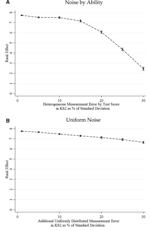
Rank estimate with different types of additional noise in the baseline score
Notes: These figures plot the mean rank estimate from 1,000 simulations of Specification 1 with increasing additional measurement error added to student baseline test scores. The measurement error for each student within a student is independently drawn. The error bars represent the 2.5th and the 97.5th percentiles from the sampling distribution of beta for each measurement error level. The extent of measurement error in Panel A is increasing linearly in distance from the 50th percentile in the national test score distribution, such that students at the 50th percentile experience no measurement error, while students at the 1st and 100th percentile experience additional measurement error drawn from a normal distribution with a mean zero and standard deviation equal to the proportion of the standard deviation in baseline test scores represented on the X-axis. The measurement error in Panel B is drawn from a uniform distribution with mean zero and a standard deviation that is proportional to the standard deviation in baseline test scores.
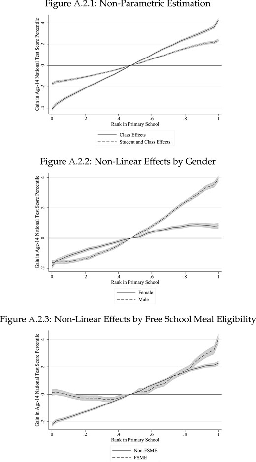
Impact of primary rank on age-14 test scores with individual effects
Notes: The panels show the impact of rank in primary school using versions of Specification 2, allowing the effect of rank to vary by ventile and including a dummy for being top or bottom of class (SSC). The reference ventile are those from the 45–50th percentiles. FSME stands for Free School Meal Eligible student. Effects obtained from estimating the effect of rank on non-FSME (female) students and the interaction term with FSME (male) students. All estimates have cubic controls for baseline test scores and condition on SSC effects and student effects. Shaded area represents 95% confidence intervals. Standard errors are clustered at the secondary school level.
