


Abstract
This paper explores the impact of product market competition on the positive relation between labor mobility (LM) and future returns. We develop a production-based model and formalize the intuition that low exposure to systematic risk in a concentrated industry limits LM’s amplifying effect on operating leverage. Therefore, the model predicts a stronger positive relation between LM and expected returns for firms in competitive industries. Consistent with the model’s prediction, we empirically find that LM predicts returns only among firms in competitive industries. This evidence suggests that the intensity of competition in firms’ product market potentially drives the positive LM-return relation. (JEL G12, G14, J69)
Authors have furnished an Internet Appendix, which is available on the Oxford University Press Web site next to the link to the final published paper online.
Labor mobility (LM) is the flexibility of workers to enter and exit an industry in response to better opportunities. Recently, this has attracted much attention in the finance literature as Donangelo (2014) shows that firms in industries employing workers whose labor skills are more portable to other industries earn higher average stock returns than those in industries where workers have less portable skills. When the performance of an industry is relatively good, it tends to attract more mobile workers. But in times of adverse productivity shocks, mobile workers tend to leave this industry. The degree of dependency on mobile labor amplifies firms’ existing exposure to productivity shocks, as outflows of mobile workers in bad times reduce cash flows. This is precisely the source of the LM premium shown in Donangelo (2014) and closely related to the risk amplification effect of labor leverage in Donangelo et al. (2019). This line of analysis, however, assumes optimistically a perfectly competitive product market environment.
Congruently, product market competition is the other well-known industrial characteristic that affects firms’ exposure to productivity shocks, but in an opposite way to the LM. For example, Dou, Ji, and Wu (2021), Hou and Robinson (2006), and Peress (2010) show that market power shields firms from nondiversifiable aggregate shocks. In other words, the operating profits of firms in more concentrated (i.e., less competitive) industries are less sensitive to the productivity shocks thanks to the benefits brought by the market power (stemming from tougher barriers to entry, low elasticity of substitution, etc.). In light of their connection with the productivity shocks, it is particularly interesting to study the juxtaposition of product market competition and LM as well as their joint asset pricing effect on the cross-section of stock returns.1 More concretely, in view of the market power to insulate firms from the productivity shocks, it is no longer clear whether the risk amplification from LM is still significant for firms in less competitive industries. In a concentrated industry, where the performance is less correlated with nondiversifiable productivity shocks, from investors’ point of view, the risk induced by inflow and outflow of mobile labor is more idiosyncratic and hedgeable. Therefore, it remains unanswered that whether LM in a concentrated industry still carries a premium in equilibrium. To the best of our knowledge, despite the first-order importance of these questions, no prior studies have attempted to answer them. These questions motivate our research in this paper and are answered in our theoretical and empirical analyses.
Guided by the work of Peress (2010), our model generalizes the mobility-production economy of Donangelo (2014) and allows for a variable measure of the product market competition. This competition measure plays a key role in quantifying the combined sensitivity to the systematic productivity shocks from the interplay between LM and product market competition. Specifically, the imperfect elasticity of substitution combined with the market concentration, which measures (the inverse of) the degree of product market competition, propagates to the demand for mobile labor, which further determines the operating profits, in the initial production stage through the price of the intermediate goods in the final product market. By construction, the mobility-production model of Donangelo (2014) is nested as a special case assuming perfect competition within our model. The solution of our model allows to study the joint effect of LM and market competition on operating leverage, which acts as a systematic risk multiplier in the firm risk. Importantly, we show that when market power within an industry is large enough, LM can barely have any effect on firms’ systematic risk. This means that the insulation induced by the market power can quickly overshadow the LM’s amplification on systematic productivity shocks. These results from our model indicate that the LM premium is more significant or exists only for firms in highly competitive industries. To verify this novel theoretical prediction, we develop a testable hypothesis that the positive LM-return relation strengthens with the intensity of product market competition.
We test our hypothesis both by independently double sorting stocks on LM and product market competition and by Fama and MacBeth (1973) cross-sectional regressions. The results from the portfolio analyses show that the positive LM-return relation exists only in competitive industries. For example, the high-minus-low LM portfolio in competitive industries delivers an economically significant value-weighted average monthly return of 0.83% (t-statistic = 3.05). The value-weighted characteristic-adjusted return of 0.79% per month on this hedge portfolio is also statistically significant, with a t-statistic of 3.76. The LM premium in competitive industries persists even after adjusting for risk using premier asset pricing models. In particular, the value-weighted average monthly abnormal returns on the hedge portfolio relative to the (unconditional) capital asset pricing model of Sharpe (1964) and Lintner (1965), the Ferson and Schadt (1996) conditional capital asset pricing model, the Fama and French (1993) three-factor model, the Fama and French (1993) and Carhart (1997) four-factor model, the Fama and French (2015) five-factor model, and the Hou, Xue, and Zhang (2015)q-factor model are 0.82%, 0.84%, 0.92%, 0.69%, 0.83%, and 0.69%, with t-statistics of 3.07, 2.96, 3.23, 2.44, 2.53, and 2.08, respectively. In contrast, the high-minus-low LM portfolio in concentrated industries generates a monthly return of –0.15% (t-statistic = –0.91). The value-weighted characteristic-adjusted return of –0.23% per month on the portfolio is also statistically insignificant (t-statistic = –1.30). Furthermore, the average monthly abnormal returns on the portfolio relative to the asset pricing models are all negative and statistically indistinguishable from zero at conventional levels. Specifically, the capital asset pricing, the conditional capital asset pricing, the three-factor, the four-factor, the five-factor, and the q-factor model alphas are, respectively, –0.09% (t-statistic = –0.58), –0.14% (t-statistic = –0.87), –0.02% (t-statistic = –0.12), –0.02% (t-statistic = –0.13), –0.02% (t-statistic = –0.14), and –0.08 (t-statistic = –0.42). We also empirically verify the key mechanism of our model, in which the market power overshadows LM’s risk amplifying effect, by showing the cross-sectional variation of factor loadings on the LM-based productivity risk factor is larger (smaller) in more (less) competitive industries.
The empirical results, supporting our hypothesis, remain robust to using: the all-but-microcaps sample, which excludes stocks with a market value of equity below the 20th percentile of the NYSE market capitalization distribution; an extended sample period; unlevered returns; industry-level returns; independent double-sorted quartile or quintile portfolios; and a wide range of product market competition measures suggested in the recent literature. For example, we employ competition measures based on the data from the U.S. Census of Manufacturers (as in Bustamante and Donangelo, 2017), both private and public firms (as in Hoberg and Phillips, 2010), firm’s product market fluidity (as in Hoberg, Phillips, and Prabhala, 2014), total assets instead of net sales (as in Hou and Robinson, 2006), and price-cost margin (as in Peress, 2010).
The model’s prediction is also supported by the results from the cross-sectional regressions. After controlling for the potential effects of size, book-to-market equity, short-term reversal, momentum, and leverage, the results confirm that a significantly positive LM-return relation prevails only for firms in competitive industries. For example, the average slope estimates of returns on LM are 0.46 (t-statistic = 4.74) and 0.09 (t-statistic = 1.39), respectively, in competitive and concentrated industries. Importantly, the average spread between the slope estimates of returns on LM in competitive and concentrated industries is 0.37, which is statistically significant with a t-statistic of 3.01. The results remain qualitatively similar, when we conduct cross-sectional regression analyses using: the all-but-microcaps sample; an extended sample period; and different measures of product market competition. In a separate cross-sectional regression analysis, we also create interaction terms involving market competition dummy variables. After controlling for firm-level attributes, such as size, book-to-market equity, short-term reversal, momentum, and leverage, the results remain robust and support our theoretical model’s prediction of a stronger LM-return relation among firms in competitive industries. For example, we find that, all else being equal, a one-standard deviation increase in LM is associated with 24 basis points higher future returns per month for firms in competitive industries relative to all other firms. A qualitatively similar finding emerges when we run panel data regressions.
Our paper contributes to two strands of literature. First, our model belongs to the burgeoning literature discussing economic mechanisms that generate labor-induced operating leverage. The general equilibrium model by Danthine and Donaldson (2002) is one of the first to articulate a mechanism in which operating leverage induced by the priority status of wage claims magnifies the risk properties of the residual payments to firm owners and justifies a substantial risk premium. Favilukis and Lin (2016) develop a general equilibrium model to examine the quantitative effect of sticky wages and labor leverage on the equity premium and the value premium. Along this line of research, Donangelo et al. (2019) provide theoretical support and empirical validation that firm-level labor share acts as a proxy for firm-level labor leverage. Our model is most close to Donangelo (2014), who shows that labor flows make bad times worse for shareholders through the LM-induced operating leverage. But different from Donangelo (2014), we focus on the more plausible case of imperfect competition.
Second, our paper is related to the theoretical studies linking industrial organization to financial markets. Aguerrevere (2009) explores the opposing effects of market competition and industry growth on expected returns. Opp, Parlour, and Walden (2014) emphasize that market competition is linked with market efficiency in a very complex way. Bustamante and Donangelo (2017) study the impact of market competition on systematic risk through the operating leverage, the entry threat, and the risk feedback channels with opposing effects. Our model is also closely related to Peress (2010), who investigates the interplay between competition in the product market and information asymmetries in the equity market. We adopt the two-sector (a final and an intermediate goods sector) economy setup of Peress (2010) in our model. Other recent studies that are broadly related to our paper include Corhay, Kung, and Schmid (2020) and Loualiche (Forthcoming). By building general equilibrium models with endogenous firm entry, both these papers examine the interaction between product market competition and asset prices. Our paper is also related more generally to Chen et al. (2021) and Dou, Ji, and Wu (2021). Chen et al. (2021) study the dynamic interactions between endogenous strategic competition and financial distress. Dou, Ji, and Wu (2021) develop an industry-equilibrium model with dynamic strategic competition to examine the joint fluctuations in aggregate discount rates, profitability, market competition intensity, and asset prices.
The uniqueness of our contribution is from the fact that we contribute to the joint venue of these two important strands of literature. The novelty of our continuous-time model lies in the analytical resolution of asset pricing implications from the interplay between LM and product market competition. To the best of our knowledge, we are the first to show, both theoretically and empirically, that market competition has a nontrivial effect on risk and return profiles of firms in high-mobility industries. In other words, the intensity of competition in firms’ product market drives a significant portion of the positive LM-return relation. This novel finding contributes to the growing subset of the asset pricing literature that investigates the interaction effect of firm characteristics on expected stock returns. Specifically, some recent papers documenting the important role that product market competition plays in explaining other cross-sectional asset pricing anomalies include Deng (2019, profitability), Dou, Ji, and Wu (2021, 2022, profitability), Giroud and Mueller (2011, corporate governance), and Gu (2016, research and development investment). In this context, we provide robust evidence of another important role that competition plays in the riskiness among firms in low- and high-mobility industries. Our study also contributes to the strand of production-based asset pricing literature that links firm characteristics to expected stock returns (see, among others, Belo, Lin, and Bazdresch, 2014; Belo et al., 2017; Cochrane, 1991; Croce, 2014; Zhang, 2019, and the references therein). Taken together, our theoretical model and strong supporting evidence improve the understanding of the joint issues across the industrial organization, and the labor and financial markets.
1. The Model
In this section, we derive a partial equilibrium model characterizing the role of product market competition in the positive relation between LM and expected stock returns. Building on the work of Peress (2010), the model introduces the more plausible case of imperfect competition to the mobility-production model developed by Donangelo (2014), which in fact assumes a perfectly competitive product market environment. Below, we outline the environment of our dynamic model and present the mechanism underlying the model’s testable prediction.
1.1 Output integrating labor and competition
We integrate LM and market competition by extending the mobility-production economy setup of Donangelo (2014) with the risk-less technology of final good production in Peress (2010).2 Specifically, we assume N firms produce intermediate goods at time t, and the final good is produced by a competitive representative final good producer (see, e.g., Corhay, Kung, and Schmid, 2020) according to a risk-less technology where is the intermediate output from ith firm and is the final output of the economy at time t, and .3 The lower , the less the elasticity of substitution between any two goods and a less competitive input market (Peress, 2010). Therefore, it measures the degree of competition in the intermediate goods sector.
Following the mobility-production economy of Donangelo (2014), we model each intermediate good output as where is the industry-specific labor skills employed by ith firm, is the output elasticity of labor, and denotes total factor productivity (TFP), which follows the diffusion process
1.2 Operating profits
Similar to Peress (2010), we use the price of the final good as the numeraire in what follows. It is worth mentioning that introducing an intermediate goods market with imperfect competition into the model economy is a convenient way to embrace imperfect competition at the whole industry level. When considering the operating profits for an average firm in the industry, we focus on the profits of each intermediate good producer.
1.2.1 Profits of the intermediate goods market
Total profits of the final good producer are given by where is the price of the ith intermediate good. The final good producers set their demand for inputs to maximize profits, . The resultant demand for each intermediate good input is . This means that when the intermediate goods market clears, the price of the intermediate good is simply
Given Equations (1) and (4), total revenue for each intermediate good producer is
We follow Donangelo (2014) and assume the only cost for the intermediate good producers is wage.4 Therefore, the profit of each intermediate good producer is given by where is the hourly wage of the labor with specific skills (see Donangelo, 2014). Each intermediate good producer sets her demand for labor to maximize profits, taking the wage, , as given. The first-order condition yields the following:
From Equation (7), we can see that because of the identical technology and constant elasticity of substitution, the labor demand, , is identical for all firms, that is, for , in equilibrium. This further implies that we have and in equilibrium. Therefore, the equilibrium final output can be simplified as
Substituting (7) for into Equation (6) yields
1.2.2 Wages and labor supply
Considering N intermediate good producers with identical labor demand , the total demand for labor is . Therefore, the profit of each intermediate good producer is connected to and N as
Hourly wages per unit of general skills are exogenously given by the diffusion process
Following Donangelo (2014), we derive the equilibrium supply of the labor with specific skills. Specially, labor markets are composed of a continuum of workers with permanent occupations based on their endowed composition of labor skills. The occupations, labeled by the index in decreasing order of labor skill specialty, are modeled as
The parameter determines the level of generality of labor skills required by the production technology. Thus, represents the level of LM in the industry (see Donangelo, 2014). Same as , we treat as another exogenous parameter. Insignificant correlations between empirical measures of these two parameters justify this exogeniety setting. We present the empirical observations in Appendix A. At time t, given an indifference marginal occupation , labor markets are in equilibrium when all workers in occupations strictly prefer to remain inside the industry, and all workers in occupations strictly prefer to remain outside the industry; therefore, the equilibrium level of employable labor skills useful inside the industry is given by:
The equilibrium indifference marginal occupation and the resultant equilibrium level of employable labor skills are derived and summarized in the following proposition.
Given the general skill wage, , the TFP, , the average level of competition, , and the number of intermediate good producers, N, the supply of labor with specific skills in equilibrium iswhere and .
Proof. See Appendix A. ▪
Now, the equilibrium operating profit of each intermediate good producer,5, can be expressed formally as
Several comments are in order before we move on. The market competition is captured primarily by . A simple inspection of Equation (14) shows that together with , LM partially controls operating profits’ sensitivity to , which Donangelo (2014) defines as the relative productivity of the industry. Indeed, conditional on , increases operating profits’ sensitivity to systematic shocks. However, from Equation (14), we also see that more extensively than the LM, controls ’s direct connection with . This is consistent with Peress (2010), who finds that market power makes profits less sensitive to systematic shocks. More concretely, affects through three channels: (1) reflecting the source of uncertainty when there is no LM, the general productivity level is now scaled to be ; (2) reflecting the relative productivity; and (3) c reflecting ’s loading on the relative productivity due to LM. Our results show that imperfect competition (small ) not only reduces the systematic risk in both absolute (channel 1) and relative (channel 2) productivity but also limits the loading on the systematic risk in the relative productivity due to the LM (channel 3). In sum, we generalize the Donangelo (2014) model to allow for imperfect market competition, and show that the influence of LM on firms’ systematic risk is much weakened when the product market is not perfectly competitive. These effects are more directly quantified via operating leverage in Section 1.3. The following proposition formalizes the dynamics of .
Given the dynamics of and , has the following dynamicswhere and .
Proof. See Appendix A. ▪
1.3 Operating leverage as a systematic risk multiplier
Donangelo (2014) derives , which the author denotes as operating leverage, to quantify the systematic risk amplification. Note that in Donangelo (2014), is always larger than one and therefore one is subtracted from the quantity to have representing the systematic risk amplification. In our case, can be less than one (but always positive, which is shown in Proposition 3 and proven in Appendix A), we therefore define the operating leverage directly as . Note that measures the sensitivity of cash flow growth to the fundamental source of risk in a multiplier sense as opposed to the Donangelo (2014) amplification sense. Given Equation (15), the equilibrium operating leverage is expressed as
It is also important to note that Equation (13) in Donangelo (2014) is a special case of Equation (16) when , which corresponds to a perfectly competitive intermediate goods market. is increasing in when , which is generally true as wages for general skills are typically smoother than TFP (see Donangelo, 2014). This result is also consistent with Bustamante and Donangelo (2017, Proposition 1), where the authors show that the operating leverage is decreasing in concentration (which measures the inverse of market competition).6 However, different from Donangelo (2014), with the relation between and is no longer always positive and depends on the value of . We formalize these results in Proposition 3 below.
Given the dynamics of and , the definition of , and assuming , the following expressions are true:
;
; and
.
Proof. See Appendix A. ▪
Proposition 3 quantifies the effects of LM and market competition on the systematic risk multiplier. Figure 1 illustrates the results. When , we reproduce the results of Donangelo (2014). The effect of LM on the systematic risk multiplier decreases mostly with the gradual decreasing of .7 More importantly, when is small enough, can barely have any effect on the firms’ systematic risk. In other words, firms’ market power can shield their profits from systematic shocks, and this insulation quickly overshadows LM’s amplification on systematic risk. These results of the systematic risk multiplier indicate that the asset pricing implications of LM (see, e.g., Donangelo, 2014) are likely to be strong or only exist in more competitive industries. Indeed, we find empirically that, in the cross-sectional dimension, in competitive industries, shocks are amplified by LM, but in concentrated industries, they are not (see Table A1 in the Appendix). In the time-series dimension, using large tariff cuts (LTC) as a proxy of increasing market competition (see Chen et al., 2021), we find that the sensitivity of firms’ profits and stock returns to a TFP factor becomes higher after the LTC and is only positively correlated with LM conditional on LTC (see Table IA3 in the Internet Appendix).8 We show in the next section that the results in Proposition 3 are directly linked to the asset pricing implications.
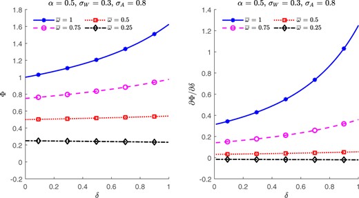
Φ versus δ
The left panel plots as a function of , and the right panel plots the first-order partial derivatives of w.r.t. . Four lines for , and 0.25 are plotted. The numerical values for the plots are shown in the subtitles.
1.4 Asset pricing implications
To explore asset pricing implications, we derive the value of a representative unlevered firm whose operating profits are given by . Consistent with the literature (see, among others, Berk, Green, and Naik, 1999, 2004; Donangelo, 2014), we take the pricing kernel as exogenous.9 The dynamics of the pricing kernel, denoted by , are given by where is a standard Wiener process representing the single source of systematic risk in the model, is the instantaneous risk-free rate, and is the market price of risk in the economy. Then, the value of the firm is the sum of all expected future operating profits (discounted properly):
Given , the firm’s instantaneous expected excess return is . The asset pricing implications of the interplay between LM and market competition can be revealed from , which is linearly linked to . The proposition below formalizes the results.
Given the dynamics of and , and assuming , the following expressions are true:
;
; and
.
Proof. See Appendix A. ▪
Part (3) of Proposition 4 combined with Part (1) of Proposition 3 indicates that LM has a positive effect on the firm’s expected excess return only when , and the degree of the effect is positively related to since . The asset pricing implication of LM diminishes when is close to zero. Therefore, we develop a testable hypothesis that the positive relation between LM and expected stock returns for firms strengthens with the degree of product market competition. In other words, the LM premium is more significant or prevails only for firms in highly competitive industries. In the following sections, we test our hypothesis and show robust evidence consistent with our theoretical model’s prediction. Although in the model we derive above we treat and N as independent parameters, we argue that can be correlated with N which captures the market concentration, for example, Herfindahl-Hirschman Index (HHI), in a more general setting. Indeed, in Appendix A, we show that in an extended version of the current model HHI is endogenously and negatively related to . This result justifies the various competition measures we use in our empirical analyses.
2. Data and Summary Statistics
This section describes the data used in the empirical analyses and the construction of product market competition and LM measures, and presents the summary statistics of relevant variables.
2.1 Data and measures of product market competition and LM
In this paper, we resort to a variety of data sources to conduct the empirical analyses. Firms’ monthly stock returns and all accounting information are sourced from the Center for Research in Security Prices (CRSP) and the Compustat Annual Industrial Files, respectively. Our preliminary sample includes all NYSE-, AMEX-, and NASDAQ-listed ordinary common stocks (CRSP share code SHRCD = 10 or 11). We filter the preliminary sample by excluding firms whose four-digit primary standard industrial classification (SIC) code is between 4900 and 4999 (regulated firms) or between 6000 and 6999 (financial firms), and firms with a nonpositive book value of equity. To account for delisting bias, we follow the approach of Shumway (1997) by imputing a return of –30% if the delisting return is missing and the delisting is performance related; however, this adjustment has no material effect on our empirical findings. The data on delisting returns are sourced from the CRSP. Our sample is restricted to the period from January 1990 to December 2016. This is due to the unavailability of data on LM for a longer sample period in the public domain, described below, which are a key ingredient of our analyses.
We focus on two samples constructed from the filtered preliminary sample, namely, the full sample and the all-but-microcaps sample. The full sample includes all NYSE-, AMEX-, and NASDAQ-listed nonfinancial and nonregulated ordinary common stocks for which both nonmissing product market competition and LM estimates in a given year are obtainable. Conversely, the all-but-microcaps sample excludes stocks, from the full sample, with an end-of-June market value of equity below the 20th percentile of the NYSE market capitalization cross-sectional distribution. Excluding microcaps (i.e., very small stocks) helps mitigating their possible undue influence on the empirical results obtained from the full sample. In an average month, the full sample comprises 2,891 firms, whereas 1,233 firms in the all-but-microcaps sample. We employ all accounting variables at the end of June of calendar year t by using accounting information available for the fiscal year ending in the calendar year 1 from the Compustat annual database. This adjustment, suggested in Fama and French (1992), provides time long enough for accounting information to be incorporated into firms’ stock prices.
Consistent with the literature (see, e.g., Giroud and Mueller, 2011; Hoberg and Phillips, 2010; Hou and Robinson, 2006), product market competition (also known as market concentration) for an industry is measured by the HHI.10 Formally, the index is defined as where is the market share of firm i in industry j in year t, is the number of firms operating in industry j in year t, and is the Herfindahl-Hirschman Index of industry j in year t.11 For each industry, we first aggregate the squared market shares of all firms in that industry in a given year t and then average the HHI values over the past 3 years. This adjustment prevents undue influence of potential data errors in the estimation of market concentration. To further improve the accuracy of the product market competition measure, we follow Hou, Xue, and Zhang (2020) and exclude an industry if the market share data are available for fewer than five firms or 80% of all firms in that industry. Throughout the main body of this paper, we compute the HHI using the market shares based on net sales (Compustat item SALE) and denote the resultant measure of product market competition by HSALE.
We also resort to six alternative measures of market competition in order to establish the robustness of the empirical findings. The first of them, denoted by , is measured per Hou and Robinson (2006), where we abstain from excluding an industry for which the market share data are available for fewer than five firms or 80% of all firms in that industry. The second of them, denoted by HAT, is the product market competition measured analogous to HSALE but using total assets (Compustat item AT) instead of net sales (Compustat item SALE). The third of them, denoted by , is obtained from Hoberg and Phillips (2010), which considers both privately held and public firms operating in a given industry by combining Compustat data with Herfindahl data from the U.S. Census Bureau and uses the fitted HHI to capture competitiveness. The fourth of them, denoted by PMF, is obtained from Hoberg, Phillips, and Prabhala (2014), which is a firm-specific competitive pressure measure (also known as firm’s product market fluidity) based on information from product descriptions contained in a firm’s 10-Ks.12 This measure captures changes in rival firms’ products relative to the firm’s products, so a higher value implies greater competitive threats faced by a firm in its product market. The fifth of them, denoted by , is obtained from the U.S. Census of Manufacturers, per Bustamante and Donangelo (2017).13 The last of them, denoted by PCM, is the firm-level price-cost margin as in Peress (2010).14 With the exception of PMF, we multiply the estimates of HSALE, , HAT, , , and PCM by minus one to simplify interpretation of the results. Hence, a higher value of these indexes/measures indicates a higher level of market competition. That is, the product market is shared by many competing firms. All competition measures are estimated and/or employed at the end of June of each year t.
The measure of LM is based on Donangelo (2014), who captures the level of interindustry dispersion of workers across occupations. Specifically, LM is constructed in two stages. In the first stage, the interindustry concentration of workers assigned to each occupation is estimated. This serves as a proxy for (the inverse of) workers’ intrinsic flexibility to switch industries. The second stage involves aggregating the occupation-level concentration measure by industry, weighted by the average annual wage expenditure corresponding to each occupation. Further details of estimating LM are provided in Donangelo (2014) and the standardized data (i.e., demeaned and rescaled to have standard deviation of one in each year) are sourced from Andrés Donangelo’s website.15 Consistent with Donangelo (2014), LM is lagged 18 months in our empirical analyses.
In the portfolio analyses, we utilize six prominent asset pricing models to compute average abnormal returns. These are the (unconditional) capital asset pricing model (CAPM) of Sharpe (1964) and Lintner (1965), the Ferson and Schadt (1996) conditional capital asset pricing (FS) model, the Fama and French (1993) three-factor (FF3) model, the Fama and French (1993) and Carhart (1997) four-factor (FFC) model, the Fama and French (2015) five-factor (FF5) model, and the Hou, Xue, and Zhang (2015)q-factor (HXZ) model. Our motivation for using the FS model is to account for possible time variation in model betas and risk premiums. The time-series data on the pricing factors (i.e., market, size, value, momentum, profitability, and investment) of the CAPM, FF3, FFC, and FF5 models, and monthly risk-free security returns are sourced from the Data Library maintained by Kenneth French.16 The time-series data on the HXZ model factors are sourced from Lu Zhang’s website.17 To compute monthly average abnormal returns on portfolios relative to the FS model, we obtain data of a set of instruments comprising the dividend yield of the Standard and Poor’s 500 Index from Robert Shiller’s website18, and the term spread between 10-year and 3-month Treasury constant-maturity yields, the Treasury-bill rate, and the default spread between BAA and AAA-rated corporate bond yields from Amit Goyal’s website.19 All of these instruments are demeaned before applying them in the time-series regressions for computing average abnormal returns on portfolios.
We use several control variables in our cross-sectional regressions. These variables include firm-level attributes, such as past 1-month return, past 1-year return skipping the last month, book-to-market equity, size, and leverage ratio. Following Fama and French (1992, 1993), we compute the book-to-market ratio, denoted by BM, at the end of June of year t as the ratio of the book value of equity at the end of the fiscal year ending in the calendar year 1 to the market value of equity at the end of December of the calendar year 1.20 In the event of a missing book value of equity, we resort to the Davis, Fama, and French (2000) book value of equity from the Data Library maintained by Kenneth French. The market value of equity, denoted by ME, is computed as absolute price per share times number of equity shares outstanding at the end of June of each year t. We obtain data on stock prices and shares outstanding from the CRSP. As in Bustamante and Donangelo (2017) and Donangelo (2014), the leverage ratio, denoted by LEV, is computed as the ratio of the book value of debt to the book value of assets minus the book value of equity plus the market value of equity at the end of June of year t.
2.2 Summary statistics
The empirical analyses begin by investigating financial and accounting characteristics across LM-sorted portfolios to help understand the data. In doing so, we allocate stocks in the full sample into three portfolios at the end of June of each year t based on the NYSE breakpoints for the bottom 30% (Low), middle 40% (Medium), and top 30% (High) of the ranked values of LM.21 The portfolios are rebalanced annually at the end of June. Panel A of Table 1 reports the time-series averages of the cross-sectional means of characteristics including HSALE, ME, BM, past 1-month return (), past 1-year return () skipping the most recent month’s return, and LEV. We see that the Low LM-sorted portfolio comprises stocks from the least competitive (or, equivalently, the most concentrated) industries, whereas the Medium LM-sorted portfolio comprises stocks from the most competitive (or, equivalently, the least concentrated) industries. Consistent with Donangelo (2014), we also find that the High LM portfolio contains stocks smaller than those comprising the other portfolios. The average market capitalization of such stocks amounts to $2,740.02 million. It is worth mentioning that both HSALE and ME exhibit a nearly inverted U-shaped relation with LM. On the contrary, average BM ratios show a monotonically decreasing relation with LM. That is, stocks in the High LM portfolio tend to be a growth stock, while stocks in the Low LM portfolio tend to be a value stock. Furthermore, past 1-month and 1-year returns increase monotonically with LM, whereas LEV displays a nearly decreasing pattern for LM-sorted portfolios.
Summary statistics
| A. Characteristics of portfolios sorted on LM | ||||||
|---|---|---|---|---|---|---|
| Portfolio | HSALE | ME | BM | LEV | ||
| Low | –0.213 | 2,946.152 | 1.059 | 1.014 | 11.301 | 0.411 |
| Medium | –0.178 | 3,421.161 | 0.746 | 1.225 | 12.150 | 0.313 |
| High | –0.206 | 2,740.021 | 0.739 | 1.411 | 16.102 | 0.320 |
| B. Portfolio excess returns | |||||
|---|---|---|---|---|---|
| Low | Medium | High | H–L | ||
| LM | VW | 0.61 | 0.66 | 0.88 | 0.27 |
| (1.77) | (2.28) | (3.02) | (1.59) | ||
| EW | 0.73 | 0.95 | 1.14 | 0.41 | |
| (1.75) | (2.20) | (2.71) | (2.33) | ||
| B. Portfolio excess returns | |||||
|---|---|---|---|---|---|
| Low | Medium | High | H–L | ||
| LM | VW | 0.61 | 0.66 | 0.88 | 0.27 |
| (1.77) | (2.28) | (3.02) | (1.59) | ||
| EW | 0.73 | 0.95 | 1.14 | 0.41 | |
| (1.75) | (2.20) | (2.71) | (2.33) | ||
| C. Excess returns of quintile portfolios | |||||||
|---|---|---|---|---|---|---|---|
| Low | 2 | 3 | 4 | High | H–L | ||
| LM | VW | 0.73 | 0.54 | 0.66 | 0.68 | 1.00 | 0.27 |
| (2.01) | (1.55) | (2.19) | (2.56) | (3.46) | (1.60) | ||
| EW | 0.72 | 0.68 | 1.11 | 0.92 | 1.19 | 0.47 | |
| (1.74) | (1.58) | (2.53) | (2.28) | (2.73) | (2.37) | ||
The sample includes all NYSE-, AMEX-, and NASDAQ-listed nonfinancial and nonregulated ordinary common stocks for which both nonmissing product market competition and labor mobility estimates in a given year t are available. There are 2,891 firms in an average month. HSALE is the product market competition measured by the Herfindahl-Hirschman Index (HHI), where for each industry, we first aggregate the squared net sales-based market shares of all firms in that industry in a given year and then average the HHI values over the past 3 years. We multiply HSALE by minus one so that a higher value indicates a higher level of product market competition. LM is the measure of labor mobility, which is computed in two stages, first at the occupation-level and then at the industry level. ME is the market value of equity (in million $) which is computed as the number of shares outstanding times the absolute price of one share at the end of June of each year . BM is the book-to-market ratio, which is computed in June of each year as the ratio of the book value of equity at the end of the fiscal year ending in the calendar year 1 to the market value of equity at the end of December of the calendar year 1. is the past 1-month return (in %). is the past 1-year return (in %) skipping the most recent month. LEV is the leverage ratio calculated as the ratio of the book value of debt to the book value of assets minus the book value of equity plus the market value of equity at the end of June of year t. At the end of June of each year t, stocks are sorted into three portfolios based on the NYSE breakpoints for the bottom 30% (Low), middle 40% (Medium), and top 30% (High) of the ranked values of LM, which is lagged 18 months, at the end of June of year t. Panel A reports the time-series averages of the cross-sectional mean characteristics of the portfolios of firms sorted by LM. Panel B (panel C) reports both the value-weighted (VW) and the equal-weighted (EW) average monthly excess returns (in %) for portfolios (quintile portfolios) sorted on LM. All portfolios are rebalanced annually at the end of June. H–L denotes the high-minus-low portfolio, that is, long stocks in the High portfolio and short stocks in the Low portfolio. Numbers in parentheses are t-statistics adjusted following Newey and West (1987). The sample period is from January 1990 to December 2016.
We then proceed to examine whether one-way sorting on LM alone generates a pattern in average excess returns over the risk-free rate. Panel B of Table 1 reports the results from such an investigation where we construct three portfolios based on the NYSE breakpoints set to the bottom 30%, middle 40%, and top 30% of the ranked values of LM at the end of June of each year t. We find that the value-weighted (equal-weighted) average monthly excess portfolio returns increase monotonically, from 0.61% (0.73%) for the Low LM portfolio to 0.88% (1.14%) for the High LM portfolio. The value-weighted (equal-weighted) average return of 0.27% (0.41%) per month for the high-minus-low LM is statistically indistinguishable (distinguishable) from zero, with a t-statistic of 1.59 (2.33). Although the value-weighted average monthly return on the high-minus-low portfolio appears to be statistically insignificant at conventional levels, the portfolio generates an economically large and statistically significant average return of 0.83% (t-statistic = 3.05) per month for stocks in competitive industries (see Table 3).
Double sorts on product market competition and labor mobility
| Low competition | High competition | |||||||
|---|---|---|---|---|---|---|---|---|
| H–L | H–L | |||||||
A. Full sample | ||||||||
| Excess return | 0.95 | 0.76 | 0.80 | –0.15 | 0.19 | 0.77 | 1.02 | 0.83 |
| (3.15) | (2.66) | (3.10) | (–0.91) | (0.50) | (2.34) | (3.02) | (3.05) | |
| Char-adj return | 0.06 | –0.21 | –0.17 | –0.23 | –0.68 | –0.12 | 0.11 | 0.79 |
| (0.38) | (–2.18) | (–1.53) | (–1.30) | (–3.97) | (–1.02) | (0.96) | (3.76) | |
| CAPM | 0.33 | 0.14 | 0.24 | –0.09 | –0.54 | 0.06 | 0.28 | 0.82 |
| (2.10) | (1.12) | (2.20) | (–0.58) | (–2.35) | (0.27) | (1.66) | (3.07) | |
| FS | 0.29 | 0.13 | 0.14 | –0.14 | –0.54 | 0.18 | 0.30 | 0.84 |
| (2.01) | (0.97) | (1.29) | (–0.87) | (–2.32) | (1.05) | (1.85) | (2.96) | |
| FF3 | 0.22 | 0.09 | 0.20 | –0.02 | –0.54 | 0.26 | 0.38 | 0.92 |
| (1.67) | (0.77) | (1.91) | (–0.12) | (–2.18) | (1.76) | (2.47) | (3.23) | |
| FFC | 0.27 | 0.15 | 0.25 | –0.02 | –0.36 | 0.44 | 0.33 | 0.69 |
| (1.91) | (1.20) | (2.53) | (–0.13) | (–1.48) | (2.31) | (2.07) | (2.44) | |
| FF5 | 0.05 | 0.00 | 0.03 | –0.02 | –0.46 | 0.43 | 0.37 | 0.83 |
| (0.37) | (0.00) | (0.25) | (–0.14) | (–1.79) | (2.25) | (2.15) | (2.53) | |
| HXZ | 0.17 | 0.07 | 0.09 | –0.08 | –0.30 | 0.58 | 0.39 | 0.69 |
| (1.08) | (0.50) | (0.81) | (–0.42) | (–1.00) | (2.88) | (1.99) | (2.08) | |
B. All-but-microcaps sample | ||||||||
| Excess return | 0.77 | 0.87 | 0.93 | 0.16 | 0.49 | 0.93 | 1.33 | 0.84 |
| (2.21) | (2.86) | (2.74) | (1.31) | (1.07) | (2.19) | (3.33) | (2.60) | |
| Char-adj return | –0.29 | –0.27 | –0.16 | 0.13 | –0.54 | –0.07 | 0.26 | 0.79 |
| (–2.84) | (–2.45) | (–1.80) | (1.08) | (–3.25) | (–0.49) | (1.67) | (3.11) | |
| CAPM | 0.03 | 0.17 | 0.17 | 0.14 | –0.47 | 0.03 | 0.45 | 0.93 |
| (0.14) | (0.92) | (1.17) | (1.18) | (–2.17) | (0.12) | (1.77) | (3.06) | |
| FS | 0.04 | 0.12 | 0.15 | 0.11 | –0.28 | 0.21 | 0.51 | 0.79 |
| (0.23) | (0.61) | (0.97) | (0.90) | (–1.12) | (0.86) | (1.80) | (2.23) | |
| FF3 | –0.15 | 0.01 | 0.03 | 0.18 | –0.46 | 0.15 | 0.53 | 0.99 |
| (–1.06) | (0.07) | (0.28) | (1.57) | (–2.17) | (0.88) | (3.16) | (3.35) | |
| FFC | 0.10 | 0.19 | 0.22 | 0.12 | –0.15 | 0.37 | 0.49 | 0.64 |
| (0.78) | (1.33) | (2.15) | (0.96) | (–0.65) | (1.86) | (3.01) | (2.17) | |
| FF5 | –0.22 | –0.15 | –0.03 | 0.19 | –0.33 | 0.50 | 0.62 | 0.95 |
| (–1.37) | (–0.95) | (–0.22) | (1.46) | (–1.18) | (2.45) | (3.78) | (2.68) | |
| HXZ | 0.03 | 0.05 | 0.11 | 0.08 | –0.03 | 0.64 | 0.68 | 0.70 |
| (0.13) | (0.24) | (0.73) | (0.56) | (–0.09) | (3.25) | (3.05) | (2.07) | |
The table reports monthly returns of portfolios sorted on product market competition and labor mobility, LM. At the end of June of each year t, stocks are sorted into three groups based on the NYSE breakpoints for the bottom 30% (Low (L)), middle 40% (Medium (M)), and top 30% (High (H)) of the ranked values of product market competition at the end of June of year t. Product market competition for an industry is measured using net sales-based market shares of all firms in that industry. Independently, stocks are sorted into three groups based on the NYSE breakpoints for the bottom 30% (L), middle 40% (M), and top 30% (H) of the ranked values of labor mobility, which is lagged 18 months, at the end of June of year t. The intersections of the product market competition and labor mobility groups result in nine portfolios. All portfolios are rebalanced annually at the end of June. The full sample includes all NYSE-, AMEX-, and NASDAQ-listed nonfinancial and nonregulated ordinary common stocks for which both nonmissing product market competition and labor mobility estimates in a given year t are available. The all-but-microcaps sample excludes stocks, from the full sample, with an end-of-June market value of equity below the 20th percentile of the NYSE market capitalization distribution and the remaining stocks are used to compute the breakpoints for product market competition and labor mobility separately. Panel A (panel B) reports the value-weighted (equal-weighted) average monthly returns (in %) on portfolios. Excess return is the portfolio return in excess of the 1-month Treasury-bill rate. Characteristic-adjusted (Char-adj) returns are computed by adjusting returns using 125 () size/book-to-market/momentum benchmark portfolios (as in Daniel et al., 1997). The alphas (in %) are estimated from the time-series regressions of portfolio excess returns on various factor models including the capital asset pricing model (CAPM) of Sharpe (1964) and Lintner (1965), the Ferson and Schadt (1996) conditional capital asset pricing (FS) model, the Fama and French (1993) three-factor (FF3) model, the Fama and French (1993) and Carhart (1997) four-factor (FFC) model, the Fama and French (2015) five-factor (FF5) model, and the Hou, Xue, and Zhang (2015),q-factor (HXZ) model. H–L is the high-minus-low portfolio. Numbers in parentheses are t-statistics adjusted following Newey and West (1987). The sample period is from January 1990 to December 2016. See also the legend to Table 1.
Panel C of Table 1 presents the results from the univariate portfolio analyses where stocks are sorted into quintile portfolios. By construction, the Low LM portfolio contains stocks below the 20th percentile of the NYSE cross-sectional distribution of LM, while the High LM portfolio contains stocks above the 80th percentile of the NYSE cross-sectional distribution of LM. We see that both the value-weighted and the equal-weighted average excess returns on portfolios generate neither a monotonically increasing nor a monotonically decreasing pattern. The high-minus-low LM portfolio delivers a value-weighted average return of 0.27% per month (t-statistic = 1.60).22 The corresponding equal-weighted average return amounts to 0.47% per month (t-statistic = 2.37). Note that the high-minus-low portfolio generates a value-weighted average return of 0.90% per month (t-statistic = 2.90) for stocks in competitive industries (see Table IA5).
3. Empirical Results
This section tests our theoretical model, which predicts that the positive LM-return relation is stronger for firms in competitive industries.23 We follow two complementary methodologies: an independent double-sorted portfolio approach and a cross-sectional regression approach.
3.1 Portfolio-level analysis
At the end of June of each year t, we assign stocks to three groups using the breakpoints for the bottom 30% (Low), middle 40% (Medium), and top 30% (High) of the ranked values of HSALE in end-of-June. Independently, we also divide stocks into three groups according to the breakpoints for the bottom 30% (Low), middle 40% (Medium), and top 30% (High) of the ranked values of LM, which is lagged 18 months, at the end of June of year t. The intersections of the three market competition and three LM groups result in nine portfolios, which are rebalanced annually at the end of June.24 Consequently, the transaction costs associated with implementing the trading strategy are expected to be low. Standard in the empirical asset pricing literature, we then obtain the value-weighted average excess returns for portfolios based on the full sample, while the equal-weighted average excess returns for portfolios based on the all-but-microcaps sample. These average excess returns allow us to provide a comprehensive picture of the relation between LM and future stock returns for firms in concentrated and competitive industries. To ensure that our results from both the full sample and the all-but-microcaps sample are robust to firm characteristics, we further compute characteristic-adjusted returns of portfolios. Specifically, following the exact procedure in Daniel et al. (1997), characteristic-adjusted returns are computed as the difference between individual stocks’ returns and 125 () size/book-to-market/momentum benchmark portfolio returns.
Table 2 summarizes the time-series averages of the cross-sectional mean characteristics of the independent double-sorted portfolios. The first two rows in panels A and B show the sorting variables LM and HSALE. As expected, LM increases monotonically when moving from the Low LM portfolio, denoted by , to the High LM portfolio, denoted by , and this pattern is similar for both the Low competition and the High competition industries. It is also observable that firms in the High competition industries tend to have lower ME, lower BM, higher past returns, and lower LEV than firms in the Low competition industries. We report the main results from the bivariate independent-sort portfolio analyses in Table 3. In panel A, which makes use of the full sample and the NYSE breakpoints to sort variables, we find that the value-weighted average monthly excess returns of LM-sorted portfolios in the High competition industries increase monotonically when moving from the Low LM portfolio, , to the High LM portfolio, . Importantly, the high-minus-low LM portfolio generates an economically large value-weighted average monthly return of 0.83%, which is highly statistically significant, with a Newey and West (1987)-adjusted t-statistic of 3.05. A monotonically increasing pattern also can be seen for the characteristic-adjusted returns when moving from the Low LM portfolio, , to the High LM portfolio, . The value-weighted characteristic-adjusted return of the high-minus-low LM portfolio is 0.79% per month, with a corresponding t-statistic of 3.76. The monthly average abnormal returns on this spread portfolio relative to the CAPM, FS, FF3, FFC, FF5, and HXZ models are also economically large and statistically distinguishable from zero; they are 0.82% (t-statistic = 3.07), 0.84% (t-statistic = 2.96), 0.92% (t-statistic = 3.23), 0.69% (t-statistic = 2.44), 0.83% (t-statistic = 2.53), and 0.69% (t-statistic = 2.08), respectively. Note that the economic magnitude of the conditional alpha (i.e., the FS model alpha) is similar to unconditional ones (i.e., the FF3, FFC, FF5, and HXZ model alphas). This suggests somewhat of a negligible time variation in the pricing model betas.
Characteristics of portfolios double-sorted on product market competition
| Low competition | High competition | |||||||
|---|---|---|---|---|---|---|---|---|
| H–L | H–L | |||||||
A. Full sample | ||||||||
| LM | –0.92 | 0.15 | 1.25 | 2.17 | –0.93 | 0.17 | 1.13 | 2.07 |
| HSALE | –0.40 | –0.40 | –0.41 | 0.00 | –0.10 | –0.09 | –0.08 | 0.02 |
| ME | 3,577.30 | 2959.38 | 3284.64 | –292.66 | 2,983.62 | 2,941.98 | 2,238.16 | –745.46 |
| BM | 0.82 | 0.91 | 0.78 | –0.04 | 0.86 | 0.61 | 0.69 | –0.17 |
| 1.01 | 0.99 | 1.14 | 0.13 | 0.81 | 1.35 | 1.53 | 0.72 | |
| 11.72 | 11.93 | 13.89 | 2.17 | 9.71 | 14.90 | 17.70 | 7.99 | |
| LEV | 0.38 | 0.39 | 0.37 | –0.01 | 0.37 | 0.23 | 0.26 | –0.10 |
B. All-but-microcaps sample | ||||||||
| LM | –0.86 | 0.29 | 1.24 | 2.10 | –0.74 | 0.23 | 1.06 | 1.80 |
| HSALE | –0.36 | –0.35 | –0.36 | 0.00 | –0.08 | –0.09 | –0.07 | 0.01 |
| ME | 6,299.22 | 6,491.35 | 6,374.82 | 75.60 | 4,864.52 | 7,285.73 | 6,202.86 | 1,338.34 |
| BM | 0.61 | 0.55 | 0.49 | –0.12 | 0.51 | 0.36 | 0.34 | –0.17 |
| 0.96 | 1.08 | 1.18 | 0.22 | 0.78 | 1.25 | 1.65 | 0.87 | |
| 11.13 | 12.40 | 13.37 | 2.24 | 8.69 | 15.09 | 19.29 | 10.61 | |
| LEV | 0.36 | 0.35 | 0.33 | –0.04 | 0.27 | 0.19 | 0.18 | –0.09 |
The table reports the time-series averages of the cross-sectional mean characteristics of the portfolios of firms sorted on product market competition and labor mobility, LM. At the end of June of each year t, stocks are sorted into three groups based on the NYSE breakpoints for the bottom 30% (Low (L)), middle 40% (Medium (M)), and top 30% (High (H)) of the ranked values of product market competition at the end of June of year t. Product market competition for an industry is measured using net sales-based market shares of all firms in that industry. Independently, stocks are sorted into three groups based on the NYSE breakpoints for the bottom 30% (L), middle 40% (M), and top 30% (H) of the ranked values of labor mobility, which is lagged 18 months, at the end of June of year t. The intersections of the product market competition and labor mobility groups result in nine portfolios. All portfolios are rebalanced annually at the end of June. The full sample in panel A includes all NYSE-, AMEX-, and NASDAQ-listed nonfinancial and nonregulated ordinary common stocks for which both nonmissing product market competition and labor mobility estimates in a given year t are available. The all-but-microcaps sample in panel B excludes stocks, from the full sample, with an end-of-June market value of equity below the 20th percentile of the NYSE market capitalization distribution and the remaining stocks are used to compute the breakpoints for product market competition and labor mobility separately. H–L is the high-minus-low portfolio. The sample period is from January 1990 to December 2016. See also the legend to Table 1.
However, we observe a completely different picture for LM-sorted portfolios in the Low competition industries (i.e., concentrated industries). For example, the value-weighted average monthly return of –0.15% on the high-minus-low LM portfolio is statistically insignificant at conventional levels (t-statistic = –0.91). The value-weighted characteristic-adjusted return of –0.23% per month on this hedge portfolio is also statistically insignificant (t-statistic = –1.30). Neither the average excess returns nor the average abnormal returns on portfolios displays a monotonically increasing pattern. For the high-minus-low LM portfolio, we also see that the value-weighted average abnormal returns relative to the six workhorse asset pricing models are all negative and statistically insignificant at conventional levels. Specifically, the CAPM, FS, FF3, FFC, FF5, and HXZ model alphas are –0.09%, –0.14%, –0.02%, –0.02%, –0.02%, and –0.08%, respectively, with t-statistics of –0.58, –0.87, –0.12, –0.13, –0.14, and –0.42. All these empirical results suggest that the positive LM-return relation exists only among firms in competitive industries. It is important to mention that the higher and statistically significant return of the high-minus-low LM portfolio of stocks in competitive industries indicates a stronger LM-return relation rather than a larger variation in the LM estimates. In fact, the spread in the LM estimates among firms with a high HSALE value in the average cross-section is 2.07, whereas it is higher at 2.17 among low HSALE firms (see Table 2).
Our empirical findings on the relation between firms’ LM and future stock returns in competitive industries are not sensitive to the all-but-microcaps sample analyzed in panel B of Table 3. For example, the equal-weighted average monthly return on the high-minus-low LM portfolio is 0.84%, which is statistically significant (t-statistic = 2.60). The equal-weighted characteristic-adjusted return on the portfolio is 0.79% per month, with a t-statistic of 3.11. Similar to that in panel A, the monthly average excess returns and the characteristic-adjusted returns of LM portfolios increase monotonically when moving from the Low LM portfolio, , to the High LM portfolio, . Moreover, the LM premium persists for firms in competitive industries even after adjusting for common risk factors using all five asset pricing models. In fact, the CAPM, FS, FF3, FFC, FF5, and HXZ model alphas on the high-minus-low LM portfolio are 0.93%, 0.79%, 0.99%, 0.64%, 0.95%, and 0.70% per month, respectively, with t-statistics of 3.06, 2.23, 3.35, 2.17, 2.68, and 2.07. On the contrary, the equal-weighted average return and the characteristic-adjusted return are, respectively, 0.16% (t-statistic = 1.31) and 0.13% (t-statistic = 1.08) per month for the high-minus-low LM-sorted portfolio in the Low competition industries. Likewise, the CAPM, FS, FF3, FFC, FF5, and HXZ model alphas remain small in magnitude and statistically insignificant at conventional levels. Specifically, they turn out to be 0.14% (t-statistic = 1.18), 0.11% (t-statistic = 0.90), 0.18% (t-statistic = 1.57), 0.12% (t-statistic = 0.96), 0.19% (t-statistic = 1.46), and 0.08% (t-statistic = 0.56), respectively. Overall, these results support our theoretical model’s prediction leading to the hypothesis that the positive LM-return manifests itself for firms in competitive industries. We also find that the results are qualitatively the same as those in Table 3 when we consider returns computed by first forming industry portfolios and then equally weighting industry returns within each competition-mobility portfolio (see Table 4).25 Furthermore, the findings in Tables 3 and 4 that the LM premium disappears, or even becomes negative, for firms in concentrated industries suggest that the positive LM-return relation identified in Donangelo (2014) is an average effect of firms from industries with different degrees of market competition. One important prediction from our theoretical model that leads to the hypothesis is Part (1) in Proposition 3, which shows that market power shields firms’ profits from systematic shocks and such insulation overshadows LM’s amplification on systematic risk. This means that the difference in the loadings on the systematic risk between high LM and low LM portfolios should be much smaller in less competitive industries. As shown in Table A2, this prediction is verified empirically. We use the (high minus low) labor mobility factor of Donangelo (2014), denoted by , as a proxy for the systematic risk.26 In Table A2, we report the factor loadings of eight double-sorted portfolios: low LM, medium LM, high LM, and high-low LM in the low competition and high competition groups. Take the full sample as an example (panel A in Table A2), the factor loadings increase monotonically with the LM in both groups, but the pattern is much stronger in the high competition group: the H-L factor loading is 1.08 (t-statistic = 12.84) in the high competition group as opposite to that being 0.38 (t-statistic = 6.17) in the low competition group. This pattern is fairly robust in the all-but-microcaps sample and to controlling for the market excess return factor of the CAPM.
Double sorts on product market competition and labor mobility: Industry-level returns
| Low competition | High competition | |||||||
|---|---|---|---|---|---|---|---|---|
| H–L | H–L | |||||||
A. Full sample | ||||||||
| Excess return | 0.67 | 0.84 | 0.70 | 0.03 | 0.34 | 0.86 | 1.06 | 0.72 |
| (1.90) | (2.44) | (2.29) | (0.14) | (1.04) | (2.63) | (3.74) | (4.18) | |
| Char-adj return | –0.36 | –0.36 | –0.29 | 0.07 | –0.39 | –0.24 | 0.16 | 0.55 |
| (–1.74) | (–2.58) | (–2.23) | (0.36) | (–3.29) | (–1.90) | (1.44) | (4.35) | |
| CAPM | 0.05 | 0.14 | 0.07 | 0.02 | –0.32 | 0.20 | 0.44 | 0.76 |
| (0.19) | (0.79) | (0.43) | (0.09) | (–1.58) | (1.10) | (2.27) | (4.04) | |
| FS | –0.03 | 0.09 | –0.01 | 0.02 | –0.33 | 0.15 | 0.34 | 0.66 |
| (–0.11) | (0.46) | (–0.08) | (0.07) | (–1.90) | (0.83) | (1.76) | (3.74) | |
| FF3 | –0.10 | –0.02 | –0.04 | 0.06 | –0.47 | 0.03 | 0.30 | 0.77 |
| (–0.43) | (–0.15) | (–0.27) | (0.27) | (–3.17) | (0.20) | (1.99) | (3.91) | |
| FFC | 0.05 | 0.14 | 0.02 | –0.04 | –0.42 | 0.18 | 0.37 | 0.79 |
| (0.26) | (0.90) | (0.12) | (–0.18) | (–2.74) | (1.28) | (2.57) | (3.93) | |
| FF5 | –0.18 | –0.08 | –0.20 | –0.01 | –0.58 | –0.12 | 0.11 | 0.68 |
| (–0.76) | (–0.50) | (–1.29) | (–0.06) | (–3.71) | (–0.76) | (0.72) | (3.47) | |
| HXZ | 0.01 | 0.11 | –0.12 | –0.13 | –0.48 | 0.04 | 0.24 | 0.72 |
| (0.04) | (0.63) | (–0.69) | (–0.55) | (–2.78) | (0.17) | (1.37) | (3.37) | |
B. All-but-microcaps sample | ||||||||
| Excess return | 0.75 | 1.02 | 0.81 | 0.07 | 0.44 | 0.83 | 1.16 | 0.72 |
| (2.31) | (3.17) | (2.64) | (0.37) | (1.30) | (2.36) | (3.50) | (4.26) | |
| Char-adj return | –0.23 | –0.15 | –0.22 | 0.01 | –0.45 | –0.28 | 0.09 | 0.54 |
| (–1.27) | (–1.27) | (–1.84) | (0.04) | (–4.15) | (–2.21) | (0.78) | (3.90) | |
| CAPM | 0.07 | 0.29 | 0.18 | 0.11 | –0.25 | 0.10 | 0.44 | 0.70 |
| (0.29) | (1.54) | (0.97) | (0.65) | (–1.22) | (0.49) | (2.12) | (4.14) | |
| FS | 0.00 | 0.31 | 0.12 | 0.12 | –0.25 | 0.04 | 0.38 | 0.63 |
| (0.01) | (1.48) | (0.69) | (0.65) | (–1.29) | (0.18) | (1.93) | (3.80) | |
| FF3 | –0.11 | 0.14 | 0.03 | 0.14 | –0.44 | –0.11 | 0.26 | 0.71 |
| (–0.59) | (0.90) | (0.23) | (0.80) | (–3.00) | (–0.74) | (1.83) | (4.39) | |
| FFC | 0.06 | 0.26 | 0.08 | 0.02 | –0.33 | 0.09 | 0.38 | 0.72 |
| (0.34) | (1.76) | (0.59) | (0.12) | (–2.39) | (0.71) | (2.76) | (3.89) | |
| FF5 | –0.24 | 0.02 | –0.19 | 0.05 | –0.56 | –0.27 | 0.05 | 0.61 |
| (–1.18) | (0.14) | (–1.38) | (0.28) | (–3.50) | (–1.81) | (0.40) | (3.57) | |
| HXZ | –0.02 | 0.13 | –0.09 | –0.07 | –0.47 | –0.07 | 0.27 | 0.73 |
| (–0.08) | (0.73) | (–0.59) | (–0.31) | (–2.45) | (–0.31) | (1.70) | (3.86) | |
The table reports monthly returns of portfolios sorted on product market competition and labor mobility, LM. The setup is the same as in Table 3, except that the results are based on returns computed by first forming (three-digit SIC code) industry portfolios, and then equally weighting industry returns within each competition-mobility portfolio. Product market competition for an industry is measured using net sales-based market shares of all firms in that industry. The full-sample includes all NYSE-, AMEX-, and NASDAQ-listed nonfinancial and nonregulated ordinary common stocks for which both nonmissing product market competition and labor mobility estimates in a given year t are available. The all-but-microcaps sample excludes stocks with an end-of-June market value of equity below the 20th percentile of the NYSE market capitalization distribution and the remaining stocks are used to compute the breakpoints for product market competition and labor mobility separately. For each portfolio in panel A (panel B), individual stock excess and adjusted returns are first value-weighted (equal-weighted) averaged within each industry comprising the portfolio, and then equal-weighted averaged across industries within the same portfolio. Excess return of a stock is the return in excess of the 1-month Treasury-bill rate. Characteristic-adjusted (Char-adj) returns of a stock are computed by adjusting returns using 125 () size/book-to-market/momentum benchmark portfolios (as in Daniel et al., 1997). The alphas (in %) are estimated from the time-series regressions of portfolio excess returns on various factor models including the capital asset pricing model (CAPM) of Sharpe (1964) and Lintner (1965), the Ferson and Schadt (1996) conditional capital asset pricing (FS) model, the Fama and French (1993) three-factor (FF3) model, the Fama and French (1993) and Carhart (1997) four-factor (FFC) model, the Fama and French (2015) five-factor (FF5) model, and the Hou, Xue, and Zhang (2015),q-factor (HXZ) model. H–L is the high-minus-low portfolio. Numbers in parentheses are t-statistics adjusted following Newey and West (1987). The sample period is from January 1990 to December 2016. See the legends to Tables 1 and 3.
Cross-sectional regressions
| Intercept | ln(BM) | ln(ME) | LEV | LM | |||
|---|---|---|---|---|---|---|---|
A. Full sample | |||||||
| Low | 1.05 | 0.42 | 0.24 | 0.45 | 0.01 | –0.24 | 0.09 |
| (2.15) | (0.74) | (0.59) | (5.61) | (0.10) | (–0.55) | (1.39) | |
| High | 2.01 | –1.64 | 0.08 | 0.42 | –0.11 | –0.53 | 0.46 |
| (2.64) | (–3.31) | (0.26) | (4.46) | (–1.41) | (–1.22) | (4.74) | |
| High–Low | 0.95 | –2.06 | –0.16 | –0.03 | –0.11 | –0.29 | 0.37 |
| (2.42) | (–3.57) | (–0.72) | (–0.40) | (–2.59) | (–0.71) | (3.01) | |
B. All-but-microcaps sample | |||||||
| Low | 0.87 | –0.25 | 0.25 | 0.19 | –0.02 | 0.23 | 0.07 |
| (1.78) | (–0.32) | (0.53) | (1.74) | (–0.50) | (0.54) | (1.28) | |
| High | 1.36 | –1.24 | 0.20 | 0.14 | –0.06 | 0.47 | 0.37 |
| (2.02) | (–1.64) | (0.56) | (1.35) | (–0.95) | (0.85) | (2.82) | |
| High–Low | 0.49 | –0.99 | –0.05 | –0.05 | –0.04 | 0.24 | 0.30 |
| (1.03) | (–1.30) | (–0.19) | (–0.48) | (–0.84) | (0.44) | (2.61) | |
The table reports the time-series average slope and intercept coefficient estimates from the Fama and MacBeth (1973) cross-sectional regressions. At the end of June of each year t, stocks are sorted into three groups based on the NYSE breakpoints for the bottom 30% (Low), middle 40% (Medium), and top 30% (High) of the ranked values of product market competition at the end of June of year t. Product market competition for an industry is measured using net sales-based market shares of all firms in that industry. Then, in each month from July of year t to June of year 1 for the Low (High) competition industries, we run a cross-sectional regression of monthly returns on lagged variables including past 1-month return (), past 1-year return skipping the most recent month (), the natural logarithm of market value of equity (ln(ME)), the natural logarithm of book-to-market ratio (ln(BM)), leverage ratio (LEV), and labor mobility (LM), which is lagged 18 months. The full sample, in panel A, includes all NYSE-, AMEX-, and NASDAQ-listed nonfinancial and nonregulated ordinary common stocks for which both nonmissing product market competition and labor mobility estimates in a given year t are available. The all-but-microcaps sample, in panel B, excludes stocks, from the full sample, with an end-of-June market value of equity below the 20th percentile of the NYSE market capitalization distribution and the remaining stocks are used to compute the breakpoints for product market competition. High–Low is the time-series average of the difference in slope or intercept coefficient estimates between the High and Low competition industries. Numbers in parentheses are t-statistics adjusted following Newey and West (1987). All independent variables (with the exception of LM) are winsorized at the 1% and 99% levels on a monthly basis prior to running the regressions. The sample period is from January 1990 to December 2016. See the legend to Table 1.
To evaluate the robustness of our preceding empirical findings over time, we also plot the value-weighted and equal-weighted cumulative log returns on the high-minus-low LM portfolios for the Low and High market competition industries in Figure 2. We see that cumulative returns only on the high-minus-low LM portfolio of stocks in competitive industries steadily increase throughout the sample period between July 1992 and December 2016. This evidence suggests that the power of LM to predict future stock returns in the cross-section persists over time only for firms in competitive industries. Taken together, the empirical results in Tables 3 and 4 and Figure 2 provide significant evidence that the positive relation between the firm’s LM and the future stock returns strengthens with the intensity of product market competition.
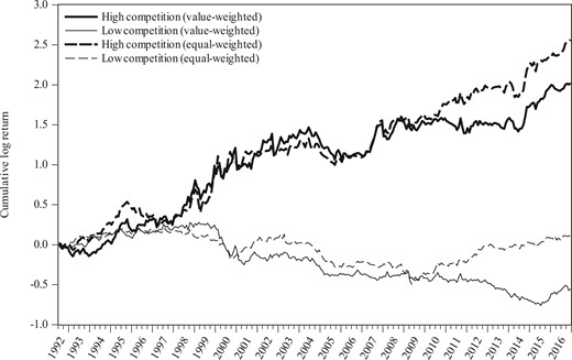
Returns on high-minus-low labor mobility portfolios
The figure plots the value-weighted and equal-weighted cumulative log returns on the high-minus-low labor mobility portfolios in the Low and High product market competition industries. The value-weighted portfolio returns are computed based on the full sample, whereas the equal-weighted portfolio returns are computed based on the all-but-microcaps sample. The sample spans July 1992 to December 2016. See also the legends to Tables 1 and 3.
3.2 Cross-sectional regressions
We also test our hypothesis by conducting the Fama and MacBeth (1973) cross-sectional regressions of monthly stock returns on lagged LM estimates and other lagged firm-level characteristics known to predict returns. Similar to that of the portfolio approach, we first sort stocks into three market competition groups according to the breakpoints for the bottom 30% (Low), middle 40% (Medium), and top 30% (High) of the ranked values of HSALE at the end of June of each year t. Then, in each month from July of year t to June of year 1, we run the following cross-sectional regressions for the Low and High competition industries separately: where R is the monthly returns from July of year t to June of year 1 on an individual stock, is the past one-month return, is the (cumulative average) return over the past 12 months skipping the most recent month’s return, ln(ME) is the natural logarithm of market value of equity, ln(BM) is the natural logarithm of book-to-market ratio, and LEV is the leverage ratio. Labor mobility, LM, is lagged 18 months, at the end of June of year t. We include , , BM, ME, and LEV as control variables to simultaneously account for the potential effects of short-term reversal, medium-term price momentum, book-to-market ratio, size, and leverage ratio on the cross-section of future stock returns. With the exception of LM, we also winsorize all explanatory variables at the 2% level (1% in each tail of the distribution) on a monthly basis prior to running the cross-sectional regressions. This help reduce possible undue influence of outlier observations on the empirical results.
In Table 6, we present the time-series average slope and intercept coefficient estimates, from the Fama and MacBeth (1973) cross-sectional regressions, along with their time-series t-statistics. To demonstrate that the LM premium increases with the level of market competition, we further report the time-series averages of the differences in slope and intercept coefficient estimates between the High and Low product market competition industries. In panel A, which utilizes the full sample and the NYSE breakpoints to sort on HSALE, we notice that the estimated average coefficient of 0.46 (t-statistic = 4.74) on LM for stocks in the High competition industries is much larger (both economically and statistically) than that of 0.09 (t-statistic = 1.39) for stocks in the Low competition industries. The average spread between the estimated slope coefficients for LM for stocks in the High competition and the Low competition industries is 0.37, which is also highly statistically significant, with a t-statistic of 3.01.
Cross-sectional regressions with product market competition dummies
| Intercept | ln(BM) | ln(ME) | LEV | LM | ||||||
|---|---|---|---|---|---|---|---|---|---|---|
A. Full sample | ||||||||||
| 1.59 | –0.55 | 0.04 | 0.40 | –0.07 | –0.28 | 0.19 | ||||
| (2.53) | (–1.22) | (0.11) | (4.68) | (–1.11) | (–0.71) | (3.30) | ||||
| 1.59 | –0.55 | 0.03 | 0.40 | –0.07 | –0.21 | 0.24 | –0.17 | –0.18 | ||
| (2.53) | (–1.24) | (0.09) | (4.77) | (–1.06) | (–0.56) | (3.29) | (–1.66) | (–1.66) | ||
| 1.40 | –0.58 | 0.04 | 0.42 | –0.06 | –0.14 | 0.12 | 0.24 | 0.27 | ||
| (2.38) | (–1.31) | (0.10) | (5.20) | (–1.00) | (–0.37) | (2.09) | (2.65) | (2.34) | ||
| 1.37 | –0.58 | 0.03 | 0.42 | –0.06 | –0.11 | 0.15 | 0.21 | –0.08 | 0.27 | –0.03 |
| (2.30) | (–1.34) | (0.07) | (5.22) | (–0.98) | (–0.29) | (1.97) | (2.07) | (–0.67) | (2.30) | (–0.27) |
B. All-but-microcaps sample | ||||||||||
| 1.17 | –0.55 | 0.14 | 0.16 | –0.05 | 0.21 | 0.17 | ||||
| (2.08) | (–0.84) | (0.33) | (1.71) | (–0.94) | (0.52) | (3.04) | ||||
| 1.18 | –0.56 | 0.14 | 0.17 | –0.04 | 0.27 | 0.23 | –0.15 | –0.12 | ||
| (2.10) | (–0.86) | (0.34) | (1.78) | (–0.89) | (0.69) | (2.92) | (–1.58) | (–1.36) | ||
| 1.05 | –0.59 | 0.14 | 0.18 | –0.04 | 0.32 | 0.11 | 0.26 | 0.18 | ||
| (1.95) | (–0.92) | (0.33) | (1.95) | (–0.82) | (0.84) | (1.98) | (2.09) | (1.49) | ||
| 1.07 | –0.60 | 0.13 | 0.18 | –0.04 | 0.33 | 0.13 | 0.24 | –0.05 | 0.16 | –0.06 |
| (1.96) | (–0.95) | (0.31) | (2.00) | (–0.82) | (0.87) | (1.84) | (1.99) | (–0.52) | (1.25) | (–0.62) |
The table reports the time-series averages of the coefficient estimates from the Fama and MacBeth (1973) cross-sectional regressions. At the end of June of each year t, dummy variables are created by sorting stocks into three groups based on the NYSE breakpoints for the bottom 30% (Low), middle 40% (Medium), and top 30% (High) of the ranked values of product market competition at the end of June of year t. Product market competition for an industry is measured using net sales-based market shares of all firms in that industry. Then, in each month from July of year t to June of year 1, we run a cross-sectional regression of monthly returns on lagged variables including past 1-month return (), past 1-year return skipping the most recent month (), the natural logarithm of market value of equity (ln(ME)), the natural logarithm of book-to-market ratio (ln(BM)), leverage ratio (LEV), labor mobility (LM), which is lagged 18 months, and product market competition dummy and interaction variables. () is a dummy variable equal to one for stocks in the High (Low) competition industries in a given month and is zero otherwise. The full sample, in panel A, includes all NYSE-, AMEX-, and NASDAQ-listed nonfinancial and nonregulated ordinary common stocks for which both nonmissing product market competition and labor mobility estimates in a given year t are available. The all-but-microcaps sample, in panel B, excludes stocks, from the full sample, with an end-of-June market value of equity below the 20th percentile of the NYSE market capitalization distribution and the remaining stocks are used to compute the breakpoints for product market competition. Numbers in parentheses are t-statistics adjusted following Newey and West (1987). All continuous independent variables (with the exception of LM) are winsorized at the 1% and 99% levels on a monthly basis prior to running the cross-sectional regressions. The sample period is from January 1990 to December 2016. See also the legend to Table 1.
When the all-but-microcaps sample is examined in panel B, we find that the results are very similar to those based on the full sample in panel A. The average coefficient estimates on LM are 0.07 (t-statistic = 1.28) and 0.37 (t-statistic = 2.82), respectively, for stocks in the Low and High product market competition industries. More importantly, the estimated average slope spread of 0.30 on LM is statistically significant, with a t-statistic of 2.61. In summary, our results from a series of monthly Fama and MacBeth (1973) cross-sectional regressions in Table 6 indicate that after controlling for the effects of firm characteristics, such as size, book-to-market ratio, momentum, short-term reversal, and leverage, the positive relation between LM and future stock returns is much stronger for firms in competitive industries.27 In fact, the existence of a significantly positive LM-return relation for firms only in competitive industries is consistent with our previous results from the independent double-sorted portfolio analyses.
3.3 Cross-sectional regressions with market competition dummies
To further examine the relation between LM and future stock returns across firms with different levels of market competition, we run the Fama and MacBeth (1973) cross-sectional regressions augmented with product market competition dummy and interaction variables. In particular, two market competition dummy variables are created by sorting stocks into three groups based on the breakpoints set to the 30th and 70th percentiles of the ranked values of HSALE estimated at the end of June of each year t. We then estimate the following cross-sectional regressions in each month from July of year t to June of year 1: where X is a vector of explanatory variables including , , ln(BM), ln(ME), LEV, and LM; () is a dummy variable that is equal to one for stocks in the High (Low) competition industries at the end of June of each year and is zero otherwise. Analogous to Table 6, we winsorize all but LM and dummy variables, and , at the 1% and 99% levels on a monthly basis before running the cross-sectional regressions.
We find that the results in Table 6 are consistent with our earlier findings based on independent double-sorted portfolio and cross-sectional regression approaches, respectively, in Sections 3.1 and 3.2. In panel A, for the full sample and the NYSE breakpoints, when we focus on the baseline monthly cross-sectional regressions given by Equation (21), we see that LM has a significantly positive relation with future stock returns. Moving to the cross-sectional regressions specified by Equation (22), we observe that the average coefficient estimate of –0.17 on the interaction variable is marginally statistically significant, with a t-statistic of –1.66. The sum of the average coefficient estimates on LM and is 0.07 (t-statistic = 1.14). This shows the absence of a significantly positive LM-return relation for firms in concentrated industries. Analyzing the cross-sectional regressions specified by Equation (23), we find an estimated average coefficient for the interaction variable of 0.24, which is both economically and statistically significant at conventional levels (t-statistic = 2.65). Since LM is standardized, the magnitude of this coefficient estimate implies that, all else being equal, a one-standard deviation increase in LM is associated with a future stock return per month for firms in the High competition industries that is 24 basis points higher than for firms in all other groups. Also, the slope estimate of returns on LM for stocks in the High competition industries (i.e., the sum of the average coefficients for LM and ) is 0.36, with a t-statistic of 3.96. For the cross-sectional regressions specified by Equation (24), we notice that the average coefficient estimates on the interaction variables and are, respectively, –0.08 (t-statistic = –0.67) and 0.21 (t-statistic = 2.07). Collectively, these results based on the full sample provide evidence supportive to our hypothesis that the positive LM-return relation strengthens with the level of product market competition.
Turning now to the monthly cross-sectional regressions using the all-but-microcaps sample in panel B of Table 6, we also find that the results are qualitatively similar to those obtained using the full sample. For example, the average coefficient estimate of 0.17 on LM from the baseline cross-sectional regressions (i.e., Equation (21)) is statistically significant (t-statistic = 3.04). For the cross-sectional regressions given by Equation (22), the average coefficient for the interaction variable is –0.15 (t-statistic = –1.58). Moreover, the sum of coefficient estimates on LM and is 0.08, which is economically small and statistically insignificant, with a t-statistic of 1.43. All of these results suggest that LM has no significantly positive effect on future stock returns for firms in concentrated industries. In the case of cross-sectional regressions specified by Equation (23), we notice that the average coefficient estimate of 0.26 on the interaction variable is statistically significant, with a t-statistic of 2.09. Economically this means that, all else being equal, a one-standard deviation increase in LM is associated with a future stock return per month for firms in the High competition industries that is 26 basis points higher than that for all firms in the Medium and Low competition industries. Notably, the sum of the average coefficient estimates on LM and is 0.37, with a t-statistic of 2.77. Finally, for the monthly cross-sectional regressions given by Equation (24), we find that the average coefficient estimates on the interaction variables and are –0.05 (t-statistic = –0.52) and 0.24 (t-statistic = 1.99), respectively. Taken together, consistent with our hypothesis, the results in panels A and B of Table 6 clearly show that the power of LM to predict future stock returns is much stronger for the cross-section of firms in competitive industries.28 Furthermore, Table IA11 in the Internet Appendix shows that the results are qualitatively the same as those in Table 6 when we run panel data regressions instead of the periodic cross-sectional regressions.
3.4 Evidence from an extended sample
Because of the lack of availability of data on LM estimates for a longer period of time, our preceding empirical analyses are based on a restrictive sample that starts in January 1990 and ends in December 2016. Hence, one may argue that the findings in this paper are specific to the relatively short sample period under investigations. In this section, we address this concern by reporting the results from independent double-sorted portfolio analyses as in Section 3.1 but using a longer sample that covers the period from January 1973 to December 2016. Specifically, we follow Donangelo (2014) in this regard and extend the baseline sample backward by setting the LM estimates in 1973 to 1989 equal to those estimated for 1990.29 Overall, the results in Table 7 suggest a significantly positive LM-return relation for firms only in competitive industries, which is supportive to our hypothesis. For example, in panel A for the full sample, the high-minus-low LM portfolio in the High competition industries generates a value-weighted average monthly return (value-weighted characteristic-adjusted return) of 0.39% (0.44%), which is statistically significant, with a t-statistic of 2.68 (2.82). The monthly average abnormal returns on this portfolio relative to the asset pricing models are also statistically distinguishable from zero. However, the high-minus-low LM portfolio in the Low competition industries generates statistically insignificant value-weighted average monthly return and value-weighted characteristic-adjusted return of –0.20% (t-statistic = –1.48) and –0.14% (t-statistic = –1.05), respectively. A qualitatively similar picture emerges for the all-but-microcaps sample, in panel B, where the high-minus-low LM portfolios delivers a statistically significant LM premium only for firms in the High competition industries. To verify the robustness of these findings, we further reestimate the Fama and MacBeth (1973) cross-sectional regressions in Table 6 using the extended sample that spans January 1973 to December 2016. The results reported in Table IA12 of the Internet Appendix strongly support our hypothesis.
Double sorts on product market competition and labor mobility: 1973–2016
| Low competition | High competition | |||||||
|---|---|---|---|---|---|---|---|---|
| H–L | H–L | |||||||
A. Full sample | ||||||||
| Excess return | 0.80 | 0.67 | 0.59 | –0.20 | 0.38 | 0.73 | 0.77 | 0.39 |
| (3.77) | (2.85) | (2.72) | (–1.48) | (1.33) | (3.24) | (3.10) | (2.68) | |
| Char-adj return | –0.28 | –0.45 | –0.42 | –0.14 | –0.63 | –0.25 | –0.19 | 0.44 |
| (–2.29) | (–5.94) | (–5.08) | (–1.05) | (–4.99) | (–2.78) | (–2.04) | (2.82) | |
| CAPM | 0.26 | 0.02 | 0.00 | –0.25 | –0.29 | 0.14 | 0.09 | 0.39 |
| (2.23) | (0.25) | (0.02) | (–1.79) | (–1.70) | (1.03) | (0.72) | (2.92) | |
| FS | 0.22 | –0.01 | –0.05 | –0.27 | –0.37 | 0.15 | 0.10 | 0.47 |
| (2.16) | (–0.06) | (–0.49) | (–1.68) | (–2.17) | (1.27) | (0.79) | (2.30) | |
| FF3 | 0.14 | 0.00 | –0.01 | –0.15 | –0.34 | 0.35 | 0.21 | 0.55 |
| (1.38) | (–0.03) | (–0.13) | (–1.07) | (–1.90) | (3.15) | (1.81) | (2.70) | |
| FFC | 0.22 | 0.06 | 0.04 | –0.18 | –0.16 | 0.50 | 0.23 | 0.39 |
| (2.09) | (0.60) | (0.49) | (–1.22) | (–0.88) | (3.63) | (1.98) | (2.01) | |
| FF5 | 0.08 | –0.12 | –0.18 | –0.26 | –0.30 | 0.50 | 0.25 | 0.56 |
| (0.81) | (–1.23) | (–1.89) | (–1.59) | (–1.55) | (3.31) | (1.82) | (2.25) | |
| HXZ | 0.21 | –0.05 | 0.01 | –0.20 | –0.11 | 0.54 | 0.46 | 0.58 |
| (1.88) | (–0.47) | (0.07) | (–1.27) | (–0.50) | (2.99) | (2.66) | (1.97) | |
B. All-but-microcaps sample | ||||||||
| Excess return | 0.77 | 0.84 | 0.77 | 0.00 | 0.58 | 0.85 | 1.09 | 0.50 |
| (3.01) | (3.27) | (2.91) | (–0.02) | (1.90) | (2.84) | (3.61) | (2.27) | |
| Char-adj return | –0.43 | –0.40 | –0.41 | 0.02 | –0.56 | –0.26 | –0.10 | 0.45 |
| (–5.47) | (–5.07) | (–5.57) | (0.26) | (–5.31) | (–2.61) | (–0.88) | (2.57) | |
| CAPM | 0.07 | 0.13 | 0.04 | –0.03 | –0.21 | 0.06 | 0.27 | 0.48 |
| (0.61) | (0.96) | (0.36) | (–0.35) | (–1.42) | (0.38) | (1.54) | (2.20) | |
| FS | 0.04 | 0.07 | 0.01 | –0.03 | –0.20 | 0.12 | 0.31 | 0.51 |
| (0.36) | (0.54) | (0.08) | (–0.35) | (–1.35) | (0.75) | (1.63) | (2.28) | |
| FF3 | –0.12 | –0.04 | –0.10 | 0.02 | –0.25 | 0.15 | 0.32 | 0.57 |
| (–1.30) | (–0.34) | (–1.09) | (0.26) | (–1.68) | (1.18) | (2.48) | (2.68) | |
| FFC | 0.07 | 0.09 | 0.06 | –0.01 | 0.03 | 0.35 | 0.34 | 0.31 |
| (0.67) | (0.80) | (0.73) | (–0.07) | (0.17) | (2.55) | (2.79) | (1.97) | |
| FF5 | –0.20 | –0.21 | –0.20 | 0.00 | –0.08 | 0.45 | 0.43 | 0.52 |
| (–1.74) | (–1.82) | (–1.95) | (–0.00) | (–0.42) | (3.05) | (3.35) | (1.98) | |
| HXZ | 0.01 | –0.04 | 0.05 | 0.04 | 0.15 | 0.58 | 0.78 | 0.63 |
| (0.07) | (–0.26) | (0.36) | (0.26) | (0.66) | (3.31) | (4.17) | (2.05) | |
The table reports monthly returns of portfolios sorted on product market competition and labor mobility, LM. The setup is the same as in Table 3, except that the sample period is from January 1973 to December 2016. The labor mobility estimates in 1973 to 1989 are set equal to those estimated for 1990 (as in Donangelo, 2014). The full sample includes all NYSE-, AMEX-, and NASDAQ-listed nonfinancial and nonregulated ordinary common stocks for which both nonmissing product market competition and labor mobility estimates in a given year t are available. The all-but-microcaps sample excludes stocks, from the full sample, with an end-of-June market value of equity below the 20th percentile of the NYSE market capitalization distribution and the remaining stocks are used to compute the breakpoints for product market competition and labor mobility separately. Panel A (panel B) reports the value-weighted (equal-weighted) average monthly returns (in %) on portfolios. Excess return is the portfolio return in excess of the 1-month Treasury-bill rate. Characteristic-adjusted (Char-adj) returns are computed by adjusting returns using 125 () size/book-to-market/momentum benchmark portfolios (as in Daniel et al., 1997). The alphas (in %) are estimated from the time-series regressions of portfolio excess returns on various factor models including the capital asset pricing model (CAPM) of Sharpe (1964) and Lintner (1965), the Ferson and Schadt (1996) conditional capital asset pricing (FS) model, the Fama and French (1993) three-factor (FF3) model, the Fama and French (1993) and Carhart (1997) four-factor (FFC) model, the Fama and French (2015) five-factor (FF5) model, and the Hou, Xue, and Zhang (2015),q-factor (HXZ) model. H–L is the high-minus-low portfolio. Numbers in parentheses are t-statistics adjusted following Newey and West (1987). See also the legend to Table 3.
4. Conclusion
This paper investigates the role of product market competition in the relation between LM and expected stock returns. To do so, we construct a production-based model in which the imperfect elasticity of substitution combined with the market concentration propagates to the demand for mobile labor, which further determines the operating profits, in the initial production stage through the price of the intermediate goods in the final product market. We show that LM can barely have any effect on the firms’ systematic risk when the market power within an industry is substantial. This implies that the insulation induced by the market power can quickly overshadow the LM’s amplification on systematic risk. Hence, our model predicts that the LM premium is stronger or exists only in highly competitive industries.
Consistent with our theoretical model’s prediction, we find robust evidence that the positive LM-return relation exists only among firms in competitive industries. This novel finding suggests that the intensity of competition in firms’ product market drives a significant portion of the positive LM-return relation. We hope that our paper enhances the understanding of the LM premium through the lens of product market competition and inspires future research combining other aspects of the industrial organization, and the labor and financial markets.
Footnotes
Empirically, we find that product market competition does not have a clear shielding effect on other shocks such the market excess return factor of the capital asset pricing model, the Fama and French (2015) five factors, and the Hou, Xue, and Zhang (2015)q factors (see the factor loadings in Table IA2 of the Internet Appendix), but has a clear shielding effect on the systematic productivity shocks identified by the (high minus low) LM factor (see Table A2). This evidence further shows the unique bond in productivity shocks shared by the product market competition and LM, highlighting the importance in studying their juxtaposition.
Our model can be pitched as an industry-equilibrium model, with the labor mobility of the industry and the competitiveness within the industry as two primitive industry characteristics. Thus, the final goods in the model should be regarded as industry-level composite goods.
Here, is strictly positive in order to avoid a degenerated economy in which the production is constant without any inputs.
We relax this assumption in Appendix A, where we add a firm-specific fixed market entry cost and endogenize the number of intermediate good producers by linking their market entering decision to their optimal profits.
Also, we can easily show that in equilibrium the average intermediate good price is explicitly linked to A, , N, and W as
It is straightforward to see that P increases with W and decreases with A. This is consistent with the fact that both W and A determine the cost of intermediate goods but in opposite ways. Although not immediately straightforward, with reasonable parameter values (e.g., , , , , and ), it also can be shown numerically that P decreases with in a reasonable range, for example, [0.3, 0.9], meaning that the average price of the intermediate goods is lower when the market is more competitive. These results are consistent with common sense and serve as additional validation on the way we model the product market competition.
Although our operating leverage result is consistent with Bustamante and Donangelo (2017), their systematic risk loading is negatively related to market competition while ours is positive, same as for the operating leverage. The Bustamante and Donangelo (2017) modeling framework is not directly comparable to ours. They assume perfect elasticity of substitution among inputs (see the industry output production function in Equation (2) of their paper), that is, . As we show here, plays a crucial role in modeling a more realistic industrial organization environment. The fact that is missing in their model casts doubt on the robustness of their theoretical predictions on the relation between systematic risk loading and product market competition.
is nonlinear (skewed U-shaped) in , with a minimal point slightly dipping below zero when is small. But most of the curve is monotonic.
Based on the coefficient estimates from Table IA3, the sensitivity of profits to TFP shocks is and that of stock returns is , where LM is the Donangelo (2014) labor mobility measure and LTC is a dummy variable that equals one if an industry experiences a large tariff cut in the last two years and is zero otherwise.
The assumption of an exogenously given pricing kernel provides the analytical tractability needed to focus on the dynamics for the relative risks of individual firms (Berk, Green, and Naik, 1999).
The elasticity of substitution in our theoretical model is not easy to measure. In the empirical study, we use HHI to measure the market competition captured by the elasticity of substitution. The numerical results in Appendix A.3 showing a clearly negative relation between HHI and justify the use of HHI as an empirical proxy for the elasticity of substitution.
As in Grullon, Larkin, and Michaely (2019), Gu (2016), Hoberg and Phillips (2010), and Hou and Robinson (2006), we use three-digit SIC codes to define industry membership.
Estimates of and PMF are sourced from the Hoberg-Phillips Data Library at http://hobergphillips.usc.edu/industryconcen.htm. Details of the estimation of and PMF can be found in Hoberg and Phillips (2010) and Hoberg, Phillips, and Prabhala (2014), respectively.
Specifically, we collect data on directly from the U.S. Census of Manufacturers publications for the years 1992, 1997, 2002, 2007, and 2012. As in Bustamante and Donangelo (2017), we forward-fill missing observations and use 2-year lags in empirical exercises. The U.S. Census provided the index at the four-digit SIC level in 1992. Since 1997, the index has been published at the six-digit NAICS level. Following Ali, Klasa, and Yeung (2009), we use NAICS correspondence tables provided by the U.S. Census to convert the index to four-digit SIC levels. More details on can be found in Bustamante and Donangelo (2017).
Details of the computation of PCM at the firm-level can be found in Peress (2010).
Details of the construction of the book value of equity can be found in Novy-Marx (2013).
Internet Appendix Table IA1 provides summary statistics of portfolios based on the all-but-microcaps sample.
In contrast to the univariate sort results based on LM in Donangelo (2014, Table V), the value-weighted average return on the high-minus-low LM portfolio is statistically insignificant at the 10% level. A possible reason is that our sample composition is a bit different from Donangelo (2014) in that we require a sample of firms with both nonmissing product market competition and LM estimates.
The results based on six alternative measures of product market competition, , HAT, , PMF, , and PCM, are qualitatively similar to those based on HSALE. To conserve space, we report these robustness check results in the Internet Appendix Tables IA13 through IA20.
To establish the robustness of our baseline empirical findings, we further conduct 44 and 55 bivariate independent-sort portfolio analyses. These additional results provided in the Internet Appendix Tables IA4 and IA5 are very similar to those reported in this paper.
The Internet Appendix provides strong evidence that the empirical results are qualitatively similar to those in Tables 3 and 4 when we conduct 44 and 55 bivariate independent-sort portfolio analyses using industry-level returns (see Tables IA6 and IA7) and use unlevered stock returns (see Table IA8).
Per our model, if an empirical factor that well represents the model’s single source of systematic risk, then we should observe the loadings on this risk factor exhibit stronger (weaker) increasing monotonic pattern with the LM in more (less) competitive industries. This is exactly what we see in Table A2 with the labor mobility factor, . Therefore, is a good proxy of the systematic risk in our model. We report the factor loadings on various other factors in Table IA2 of the Internet Appendix. We find that neither the CAPM nor the other factors we consider can reproduce this pattern, indicating that none of the traditional factors empirically represents the systematic risk in our model.
Internet Appendix Table IA9 shows that the results remain robust when stocks are sorted into five groups based on the NYSE breakpoints set to the 20th, 40th, 60th, and 80th percentiles of the ranked values of HSALE.
Internet Appendix Table IA10 shows that the results are qualitatively similar when () is equal to one for stocks in the top (bottom) 20% percentile of the ranked values of HSALE and is zero otherwise.
See Table IA.XIII in the internet appendix of Donangelo (2014). To get an idea about labor mobility transition probabilities, see also Table IA.XI of Donangelo (2014).
Appendix A
A.1 Proofs
This completes the proof of Proposition 1. ▪
Proof of Proposition 2. The following lemma is helpful for streamlining the proof.
if, then, whereand.
if , then, whereand.
Proof.
- By Itô’s lemma, we have
- and can be solved analytically with and as
▪
Therefore,
Now, we rewrite as , where . By Lemma A1, we formally have
This completes the proof of Proposition 2. ▪
Proof of Proposition 3. At the outset, it is helpful to have and .
Since , and , we have ; and
.
This completes the proof of Proposition 3. ▪
Proof of Proposition 4.
- Define . By Lemma A1, we havewhere and . Therefore,
An alternative proof can be found in the Internet Appendix of Donangelo (2014).
- , therefore,
Directly from Part (2) above and Equation (16). ▪
A.2 Evidence on Exogeneity between Market Competition and Labor Mobility
In this appendix, we show empirically that the correlation between product market competition and labor mobility, LM, is negligible. Following Peress (2010), we use the firm-level price-cost margin, PCM, to construct an empirical proxy of for individual intermediate goods. Specifically, where normCDF is the standard normal distribution CDF. This transformation ensures that the constructed is inversely related to PCM and is always within (0, 1). Similarly, we construct as , where the measure of individual LM is based on Donangelo (2014), which captures the level of interindustry dispersion of workers across occupations.
The unconditional correlation between and is only 1.5%. We also calculate the correlations conditional on year and cross-industry: in each year we calculate two correlations, one from individual and , the other from and cross-industry, where and is the average PCM within an industry, and and is the average LM within an industry. These correlations are presented in Figure A1. Over the years, these conditional correlations between and are symmetrically dispersed around zero with small absolute values. This evidence serves as an indication of no systematic relation between product market competition and labor mobility.
A.3 Extending the Model with Endogenous N
The model we drive in the main body of the paper is conditional on an exogenous number of intermediate good producers, N. In this Appendix, we endogenize N by linking the expected optimal profit of each intermediate good producer, , to their market entry decision. Specifically, the intermediate goods market is characterized by the average elasticity of substitution . There is a mass of M potential producers whose fixed entry costs are uniformly distributed across . So, the density of potential producers is . All three variables are functions of . It is sensible to expect M to be larger and to be smaller, therefore, to be larger in a more competitive market. We assume and . A potential producer only enters the market if the expected profit is higher than her fixed cost. Therefore, the equilibrium N solves the following equation where as a function of and N is given in Equation (14). as a function of can be solved numerically. We use the following settings to numerically show the endogenous relation between N and : , , , , , , and , and goes from 0.3 to 0.99. The HHI is defined as the sum of the squared market shares. In our model, each intermediate good producer has an equal market share, therefore, HHI in our model is simply . The numerical illustrations are presented in Figure A2. We can see that N (HHI) increases (decreases) with , while price and profit decrease with . The intuition is straightforward: the reduction of fixed cost overweights the reduction of profit in a higher (more competitive) market, making it appealing for more potential producers to enter the market. This pattern matches remarkably with empirical observations presented in Figure A3, where we show that an empirical measure of (constructed as the standard normal distribution CDF of the negative average price-cost margin, Peress 2010) is clearly negatively correlated with and HHI (computed using market shares based on net sales).
Appendix B. Supplementary Data
Supplementary results related to this article can be found in the Internet Appendix.
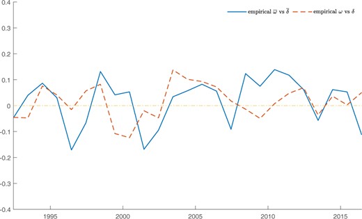
Correlation coefficients betweenandover time
The figure plots yearly cross-industry correlations between the empirical measures of and (solid line) and those between and in each industry (dashed line). The empirical measure of () for an industry is defined as the standard normal distribution CDF of (), where () is the average value of PCMs (LMs) of all firms within the industry. Industries are identified at the three-digit SIC level. The sample period is from 1992 to 2016.
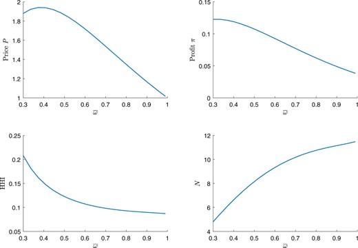
Endogenous N as a function ofalongside other key variables
The numerical settings for the plots in this figure are , , , , , , and . The top two panels plot P and against , respectively, and the bottom two panels plot HHI and N against , respectively.
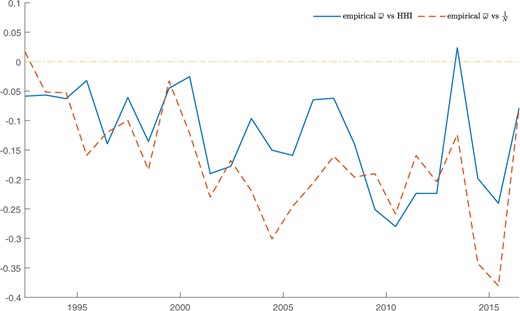
Correlation coefficients betweenand HHI andover time
The figure plots yearly cross-industry correlations between an empirical measure of and HHI (solid line), and those between the empirical measure of and the number of firms in each industry (dashed line). The empirical measure of for an industry is defined as the standard normal distribution CDF of , where is the average value of PCMs of all firms within the industry. Industries are identified at the three-digit SIC level. The sample period is from 1992 to 2016.
Labor mobility and sensitivities of profits and returns to industry shocks in subsamples split by product market competition
| Low competition (28 industries) | High competition (28 industries) | ||||
|---|---|---|---|---|---|
| Industries | Dependent variable: | Industries | Dependent variable: | High–Low | |
A. Sensitivities to | |||||
| 28 | 0.76 | 28 | 3.89 | 3.13 | |
| (1.11) | (17.30) | (4.86) | |||
| Low mobility | 14 | 0.84 | 13 | 3.40 | |
| (0.54) | (8.75) | ||||
| High mobility | 14 | 0.72 | 15 | 4.38 | |
| (1.12) | (19.08) | ||||
| High–Low | –0.12 | 0.98 | |||
| (–0.08) | (2.18) | ||||
B. Sensitivities to | |||||
| 28 | 0.95 | 28 | 3.84 | 2.89 | |
| (1.38) | (17.14) | (4.46) | |||
| Low mobility | 14 | 1.33 | 13 | 3.37 | |
| (1.66) | (8.67) | ||||
| High mobility | 14 | 0.76 | 15 | 4.31 | |
| (1.22) | (19.01) | ||||
| High–Low | –0.56 | 0.93 | |||
| (–0.38) | (2.08) | ||||
| Dependent variable: Returns | Dependent variable: Returns | ||||
C. Sensitivities to | |||||
| 28 | 0.05 | 28 | 0.27 | 0.22 | |
| (3.21) | (5.81) | (5.02) | |||
| Low mobility | 14 | 0.02 | 13 | 0.20 | |
| (1.83) | (3.63) | ||||
| High mobility | 14 | 0.08 | 15 | 0.41 | |
| (2.72) | (4.69) | ||||
| High–Low | 0.06 | 0.21 | |||
| (1.66) | (2.14) | ||||
D. Sensitivities to | |||||
| 28 | 0.08 | 28 | 0.28 | 0.20 | |
| (2.34) | (5.44) | (4.45) | |||
| Low mobility | 14 | 0.02 | 13 | 0.19 | |
| (1.77) | (3.09) | ||||
| High mobility | 14 | 0.15 | 15 | 0.43 | |
| (2.12) | (4.02) | ||||
| High–Low | 0.13 | 0.24 | |||
| (1.64) | (2.03) | ||||
The table reports the cross-sectional average slopes of univariate time-series regressions of percentage changes in industry-level profitability and (percent) industry-level returns on percentage changes in total factor productivity (TFP). Data are sourced from the Manufacturing and Nonmanufacturing KLEMS/BLS and from the OES/BLS data sets. A list of the broad industry groups used in the KLEMS/BLS data set is provided in the Internet Appendix Table IA.I of Donangelo (2014). In the first row of each panel, we assign industries into Low competition and High competition groups based on their average cross-sectional ranked values of product market competition. In the second and third rows of each panel, Low competition and High competition industry groups are further assigned to labor mobility subsamples based on their average cross-sectional ranking. Product market competition for an industry is measured using net sales-based market shares of all firms in that industry. is growth in the ratio of payments to capital over productive capital stock. is multifactor productivity growth. is the residual of time-series regressions of growth on lagged employment and productive capital growth. Numbers in parentheses are t-statistics based on Huber-White robust standard errors. The sample period is from January 1990 to December 2016. Details on the estimation of the time-series regressions can be found in Section II.D and Table IV of Donangelo (2014).
Labor mobility and market factor loadings of double-sorted portfolios
| Low competition | High competition | |||||||
|---|---|---|---|---|---|---|---|---|
| H–L | H–L | |||||||
A. Full sample | ||||||||
| factor | ||||||||
| –0.35 | –0.16 | 0.03 | 0.38 | –0.65 | –0.09 | 0.42 | 1.08 | |
| (–2.72) | (–1.40) | (0.27) | (6.17) | (–3.47) | (–0.61) | (2.32) | (12.84) | |
| MKT and factors | ||||||||
| MKT | 0.94 | 0.94 | 0.87 | –0.07 | 1.11 | 1.10 | 1.15 | 0.04 |
| (17.24) | (20.92) | (23.40) | (–1.43) | (15.45) | (10.94) | (22.87) | (0.54) | |
| –0.30 | –0.11 | 0.07 | 0.37 | –0.60 | –0.04 | 0.48 | 1.08 | |
| (–4.39) | (–2.00) | (1.08) | (6.42) | (–6.55) | (–0.31) | (7.45) | (13.10) | |
B. All-but-microcaps sample | ||||||||
| factor | ||||||||
| –0.40 | –0.21 | –0.17 | 0.23 | –0.39 | 0.10 | 0.48 | 0.87 | |
| (–2.42) | (–1.43) | (–1.14) | (4.68) | (–1.79) | (0.42) | (1.83) | (6.73) | |
| MKT and factors | ||||||||
| MKT | 1.13 | 1.07 | 1.16 | 0.03 | 1.47 | 1.38 | 1.36 | –0.11 |
| (19.18) | (32.72) | (24.03) | (0.94) | (19.99) | (13.99) | (24.64) | (–1.34) | |
| –0.34 | –0.16 | –0.11 | 0.23 | –0.32 | 0.17 | 0.55 | 0.87 | |
| (–3.92) | (–2.13) | (–1.57) | (4.63) | (–3.05) | (1.35) | (4.15) | (6.39) | |
The table reports risk factor loadings from the time-series regressions of portfolio excess returns (in Table 3) on: (1) a constant and the (high minus low) labor mobility factor of Donangelo (2014), denoted by ; and (2) a constant, , and the value-weighted market excess return (MKT) factor. Details on can be found in Donangelo (2014). The full-sample includes all NYSE-, AMEX-, and NASDAQ-listed nonfinancial and nonregulated ordinary common stocks for which both nonmissing product market competition and labor mobility estimates in a given year t are available. The all-but-microcaps sample excludes stocks with an end-of-June market value of equity below the 20th percentile of the NYSE market capitalization distribution and the remaining stocks are used to compute the breakpoints for product market competition and labor mobility separately. H–L is the high-minus-low portfolio. Numbers in parentheses are t-statistics adjusted following Newey and West (1987). The sample period is from January 1990 to December 2016. See also the legends to Tables 1 and 3.
Acknowledgements
We are grateful to Hui Chen (the editor), an anonymous referee, Guofu Zhou, Erik Loualiche, Seok Young Hong, Seung Yeon Yoo, Zhou Zhang, Di Luo, Lucio Sarno, Alex Kostakis, and Charlie Cai for many useful comments and suggestions, as well as to participants at University of Liverpool Management School Finance seminar, the 57th Annual Eastern Finance Association Meeting, the 37th International Conference of the French Finance Association, and 2021 FMA Annual Meeting.
