


Abstract
Let q be an odd prime power and D be the set of irreducible polynomials in which can be written as a composition of degree two polynomials. In this paper, we prove that D has a natural regular structure by showing that there exists a finite automaton having D as accepted language. Our method is constructive.
1. Introduction
It has been of great interest in recent years the study of irreducible polynomials which can be written as composition of degree two polynomials (see for example [1, 2, 6, 8, 9, 11, 13, 14, 15–17]). Such polynomials are also used in other contexts, see for example Rafe Jones’ construction of irreducible polynomials reducible modulo every prime [15] or the proof of [3, Conjecture 1.2] in [5]. In this paper, we explain how the theory of this class of polynomials completely fits in a general context which allows the use of powerful machinery coming from the theory of finite automata (in characteristic different from 2). In fact, we show that some irreducibility questions over finite fields can be translated into automata theoretical ones (see Definition 3.6 and Theorem 3.8). As a side result, we also obtain that the set of irreducible polynomials which can be written as the composition of degree two polynomials is naturally endowed with a regular structure given by Theorem 3.11.
Let be a finite field of odd characteristic and let be a set of monic degree two polynomials. In this paper, we consider the set to be an alphabet, and a word corresponds to the composition . The empty word naturally corresponds to . Let be the language of words whose corresponding compositions are irreducible. Our goal is to show that is a regular language by providing an automaton that accepts it. The entire theory lifts to local fields under the assumption that the set is finite and none of its elements has discriminant in the maximal ideal of the local field.
2. Distinguished sets and freedom
We include in this section some elementary facts concerning the freedom of the monoid generated by a finite set of irreducible degree two polynomials. These results will be needed in Section 3. Each polynomial can be uniquely written as for some . We define to be the distinguished set of .
We denote by the set of words over the alphabet , so is the free monoid generated by the symbols in . Let be the compositional monoid generated by , that is the smallest subset of containing and which is closed by composition.
We will denote by the natural surjective morphism of monoids which maps a word to the composition . Notice that, for an element , we will denote by the -fold composition of with itself.
In this section, we provide a computable condition to establish whether is a free monoid, which will be needed later on.
Letbe words ofof equal length. Letbe the-suffixes ofand, respectively. Then
implies
if and only iffor some.
Let us now prove (ii). If , by definition we have for for some . Now, by squaring and subtracting on both sides of the equality we get for some , and hence . Vice versa, if there exists such that , then (i) applies.□
Letbe words ofof equal length. Ifor, then we have thatif and only if.
One direction is trivial: if , then . For the other direction, we look at the two cases separately.
In the case , it follows from that for some . However, consists of only one element, so .
For the case , assume that , so for some . Let be the -suffixes of and . Then, since , we have that for some . As is constant, this forces , which in turn forces and hence .□
The following proposition shows that the freedom of the monoid is ensured whenever is either maximal or minimal.
Ifor, then.
Clearly, a polynomial of degree two in cannot have two distinct writings in terms of compositions. Let be a polynomial in of minimal degree with two different writings, that is, such that for and of positive length. From , one deduces by Proposition 2.1 that . Lemma 2.2 now gives , which implies by the minimality of .□
Ifthen.
Immediate by observing that or .□
3. An automaton for irreducible compositions
3.1. Capelli’s Lemma
In this subsection, we describe the basic tools needed to establish the main result. We start with a well-known result by Capelli, which gives a necessary and sufficient criterion to control the irreducibility of the composition of two polynomials.
Letbe a field andpolynomials. Letbe a root of. Then, is irreducible overif and only ifis irreducible overandis irreducible over.
We now use Capelli’s Lemma to produce a simple ancillary result which will help us in what follows.
Letbe monic and irreducible of even degree, and let. Then, is irreducible if and only ifis not a square in.
We are now ready to state one of the basic ingredients of the proof of the main theorem, which will allow us to ‘push’ irreducibility questions for compositions of degree two polynomials on a finite level.
Letbe monic polynomials of degree two. Writefor all. Then, is irreducible if and only if all of the following are non-squares in:
.
Clearly, is irreducible if and only if is a non-square. The rest follows by inductive application of Lemma 3.2.□
3.2. Brief interlude on Automata Theory
In this subsection, we recall the basic results needed in the next section. For the definition of deterministic finite automaton (DFA) and non-deterministic finite automaton (NFA), we refer for example to [12, Chapter 2]. Since all the automata in the paper will have a finite set of states, we will often omit the word finite.
Let be a set of symbols (an alphabet) and be the set of words over , that is the free monoid generated by it. Let us recall that a subset of is called a language. Let · be the usual binary operation in (that is, concatenation of words) and be the unary operation on languages defined by where is the smallest submonoid of containing (in the context of languages, this operation is often called Kleene star).
A language is said to be regular if it is finite or can be expressed recursively starting from finite sets using the operations (see [12] for more details). The following fact is well known.
A language is regular if and only if it is accepted by a DFA.
We will need the following fundamental results from the theory of Automata.
If a languageis accepted by a DFA or an NFA, then it is regular.
Roughly, the theorem above states that the accepted languages of NFAs do not generalize the notion of regular language.
We will also be using the notion of a partial deterministic finite automaton, which is the same as a DFA, except the transition function is actually a partial function. If, when reading a word, a required transition is not defined, the word is rejected. Clearly, a partial DFA is a special case of an NFA, so languages accepted by partial DFAs are also regular.
3.3. Putting all together: building the automaton
We first define a finite deterministic automaton using the data contained in .
The states of the automaton are given by the following:
A special start state . It is accepting.
For each , we have a distinguished state . It is accepting if is a non-square.
For each , we have a state . It is accepting if is a non-square.
For each , we have a transition .
For each and each , we have a transition .
For each and each , we have a transition .
The reason we distinguish between the states and is that they may be accepting at different times: accepts if is non-square, if is non-square. In the case that is a square in , the two are equivalent and we can identify the two types of states.
The languageof irreducible compositions is regular.
Let be the regular language over the alphabet that is accepted by the automaton reading from right to left. It is easy to see that a single letter is in if and only if is nonsquare. Furthermore, a word , , is in if and only if is nonsquare. By Proposition 3.3, it follows that the word corresponds to an irreducible polynomial if and only if each prefix , , lies in . In other words, is the language of all words whose every prefix is in .
We want to prove that is regular. To do so, let us first construct a non-deterministic automaton from by reversing all the arrows of and setting the start state of as final state of and the final states of as start states of . Observe that the accepted language of is again the language , this time reading from left to right as usual. Now we use subset construction (see for example [12, Section 2.3.5]) to generate a new deterministic automaton having the same accepted language as . Finally, we remove all non-accepting states from to obtain the partial automaton . It is easily seen that accepts exactly those words whose every prefix is accepted by , which as explained above is .□
Notice that the language accepted by the final automaton is prefix closed.
We now provide an example to see the theorem in action.
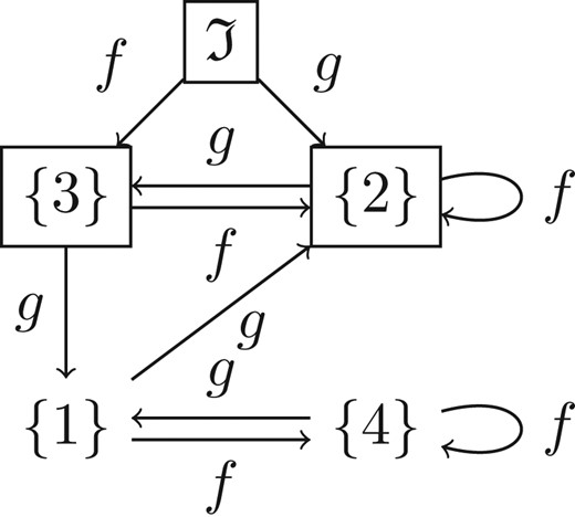
As a simple example, consider the case and with and .
We first construct the interim automaton using the method described in Definition 3.6. Since , we can identify the nodes and . Note that we have removed the node since it is not reachable from . The result is seen in Fig. 1.
After performing the transformation described in the proof of Theorem 3.8 and cutting out all unreachable states, we end up with the simple partial automaton in Fig. 2. This shows that the irreducible compositions of and are precisely those of the form , , and for .
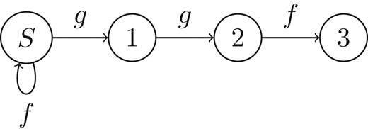
The automaton accepting for Example 3.10. All states are accepting.
Using the machinery we developed in the rest of the paper, we describe an infinite set of primes of having a finite regular structure.
Letbe a finite field of characteristic different from 2. The set of monic irreducible polynomials having coefficients inwhich can be written as a non-empty composition of degree 2 polynomials can be partitioned into a finite disjoint unionin such a way that eachis in natural bijection with the words of a regular language, which is independent of. In particular, the set of monic irreducible polynomials has a finite regular expression in terms of the elementary operations.
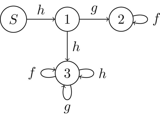
The automaton accepting for Example 3.12. All states are accepting.
Let us now describe two implications of our result in the case in which is small compared with . Recall that the iterated logarithm of a positive real number , denoted by , is the number of times the logarithm function must be iteratively applied before the result is less than or equal to .
For fixed, we can list all monic irreducible polynomials of degreewhich are compositions of degree 2 polynomials with complexity, where the implied constant depends only on.
First, we choose and write down the automaton given by Theorem 3.8. The complexity of this step is , where the implied constant clearly depends only on . Since the distinguished set is maximal, we can identify the polynomials and the words in . Now the construction is recursive: let be the set of words of of length (so polynomials of degree ). For any word and any , check if the word is accepted by the automaton : if it is, is an element in . This check takes constant time for fixed if for each element of we also store the state in which the automaton ends after reading it. As we observed in Remark 3.9, the language accepted by is prefix closed, so all the elements of can be constructed in this way. Then, constructing from costs at most .
In order to represent the elements of by coefficients, we now need to evaluate the elements of . For a single such element, if we evaluate it from inside out, this means squaring polynomials of degree and subtracting a constant each time. According to [10], such a squaring can be done in time , the total time for each element hence being .□
The reader should notice that this is much quicker than listing such polynomials by using an irreducibility test. This would have in fact complexity , where is the cost of the chosen irreducibility test for a polynomial of degree . Again, the implied constant depends on the time of constructing the automaton, which just depends on the parameter .
Another interesting fact is that (again for fixed ) we have an efficient deterministic algorithm to test irreducibility for polynomials which are a composition of degree two polynomials.
Letbe a polynomial of degreewhich is known to be a composition of monic degree two polynomials. Thencan be tested for irreducibility in time, where the implied constant depends only on.
We need to write in the form , where and , with and in .
For this, suppose we have with , where , and is a polynomial of degree . Assume is known, and we seek and . We apply the algorithm Univariate decomposition from [7, Section 2] with . This gives us the unique of degree 2 and of degree with such that . Clearly, setting , we have and . From this, it is easy to recover , , and . The algorithm Univariate decomposition takes time , again using the multiplication algorithm from [10].
Applying this repeatedly to the from the theorem will find the decomposition in time, which can then be checked for irreducibility with the automaton in time . Again, for fixed , constructing the automaton has constant complexity, independently of the degree of the polynomial we are testing.□
For fixed , testing irreducibility for a polynomial of degree using for example Rabin’s test [18] with fast polynomial operations costs .
As we already mentioned, the whole point is that our algorithm is very efficient in the regime of small fixed and large . Let us nonetheless have a quick look at the complexity with regard to . If we follow the algorithm as described in Corollary 3.15 directly, the complexity appears to be exponential in . In particular, we can expect the subset construction step to take exponential time and space.
Fortunately, it is not in fact necessary to construct the entire automaton to execute the above algorithm. Instead, we can solely construct the interim automaton from Theorem 3.8. This takes field operations, and has to be done only once for each . Then, given the decomposition of the polynomial into we can run a word through directly as follows: define as the set of accepting states of . Then, for from to , let be the set of all states such that there is an and a transition in . If at some point does not contain the initial state , we reject the word. Otherwise, we accept.
This method mirrors the reversal and subset construction from Theorem 3.8, except that only the parts that are actually used are computed. The complexity of this algorithm is easy to determine: when computing from , we can iterate over all states of the automaton and check whether the unique outgoing transition labelled ends in . Hence, each step takes only field operations, for a total cost of . Since for small the quantity dominates , the complexity in terms of -operations remains unchanged.
4. Irreducible compositions over local fields
In this final section, we will show how the results of the previous sections can be lifted, under some additional hypothesis, to polynomials over local fields. Let be a non-Archimedean local field with finite residue field of odd characteristic. Let be its ring of integers and be a uniformizer. We will denote by the reduction map . Let us start by recalling the following lemma, which we state in a weaker form, sufficient for our purposes.
See [14, Lemma 2.6].□
Letbe monic polynomials of degree 2 such that. Thenis irreducible inif and only ifis irreducible in.
.
It is clear that the hypothesis that is necessary for the claim to hold, since for example is irreducible in , while its reduction is reducible in .
Given a finite set of monic polynomials of degree two with unitary discriminant, Theorem 4.2 shows that irreducible compositions of the elements of correspond bijectively to irreducible compositions of the elements of . Therefore, if we consider as an alphabet and is the language of irreducible compositions of the elements of , we deduce immediately the following corollary.
The languageis regular.
It is enough to apply Theorem 3.8 to the language of irreducible compositions of the elements of .□
The above corollary essentially states that the theory we developed in the rest of the paper lifts entirely to local fields, at least in the case in which the elements in have unitary discriminant. It would be interesting to understand what happens when this condition is not satisfied.
5. Further research
One of the natural questions arising from the results in the present paper is whether Theorem 3.11 can be generalized to higher degree polynomials. In fact any lift of such results to polynomials of degree three or more would be of great interest, in particular because the necessary and sufficient criterion by Boston and Jones [16] (and the subsequent results on the subject such as [1, 2, 6, 8, 11]) only exists in degree two. In the context of local fields, another interesting issue arising from Theorem 4.2 of this paper is the following: how can one include singular polynomials in the generating set ? In fact, the condition on the discriminant seems to be essential. Another question arising from these results is whether it is possible to explicitly compute the generating function of the language of irreducible compositions just in terms of the coefficient of the generating polynomials. It is indeed possible to compute such a function just in terms of the obtained automata, but this would drop most of the available information. In particular, it seems that the key ingredient to address this issue is to understand the structure of the finite submonoid of maps from to which can be written as composition of degree two polynomials. More generally, many of the questions and constructions which were related just to the compositions of a single polynomial, now seem to naturally arise in this more general context, were the rigidity of finite automata theory provides assistance.
Funding
The first author was supported by Swiss National Science Foundation Grant no. 168459. The second author is thankful to Swiss National Science Foundation Grant nos. 161757 and 171248.
Acknowledgements
The authors are thankful to the anonymous referee for his suggestions, which greatly improved the content and the readability of the paper. We are especially thankful for suggesting a reference which boiled down the complexity in Corollary 3.15 from to .
