Abstract
The evolution of solitary waves governed by perturbations of the Korteweg-de Vries (KdV) equation is considered, focussing in particular on the Burgers-Korteweg-de Vries (BKdV) equation. Using matched asymptotic expansions the structure of the wave is determined for all timescales. A tail appears behind the main waveform, the structure of which is determined in the form of a convolution integral. Numerical results are presented using a pseudospectral scheme but modified so that linear terms are incorporated into an integrating factor. All details of the asymptotic structure of the waveform are validated by numerical results. Comparisons are made with earlier asymptotic analyses of decaying solitary waves.
1. Introduction
Modelling of the surface elevation of long-wavelength, small-amplitude disturbances on a fluid layer leads to the Korteweg-de Vries (KdV) equation [1]
Including uniform surface tension modifies
|$ \lambda $|, the coefficient of dispersion, but if the Bond number, which characterises the relative importance of surface tension forces, is close to a critical value, an additional fifth-order spatial derivative term arises [
2]. More recently a governing equation was derived taking account of viscous dissipation due to the base boundary condition and arbitrary stress conditions applied at the free surface [
3]. This general theory covers the case of normal electric fields [
4–6] and more general electromagnetic forcing, along with the case of surfactant transport giving rise to tangential stress at the surface. In each case the governing equation can be written as a perturbed KdV equation of the form
where the additional physical processes described above are absorbed into
|$ \mathcal{R}(f) $| term. In this paper we are concerned with solutions of these problems when the effect of these additional processes are small, that is
|$ \epsilon\ll 1 $|. Particular cases are discussed in due course, with the physical interpretation of
|$ \epsilon $| explained.
The unperturbed KdV equation is well known for having solitary wave, or soliton, solutions. The single soliton solution of (1.1) takes the form
where the propagation speed is given by
|$ C=2A $|. This has the property of constant unchanging amplitude, with the speed and width of the wave directly depending on the magnitude of the amplitude. In [
3] numerical solutions of the perturbed KdV equation were presented taking the soliton solution as an initial condition. A wide range of behaviour is seen, which can not be immediately explained in physical terms. For this reason, investigation of the case when the perturbation is small (ie
|$ \epsilon\ll 1 $|) seems to be a good starting point.
Solutions of the equation
are considered by [7, 8] for |$ \epsilon\ll 1 $|. Four different linear terms |$ \mathcal{R}(f) $| are considered covering the physical situations of magnetosonic waves damped by electron-ion collisions, ion sound waves damped by ion-neutral collisions and by electron Landau damping, and shallow water waves damped by viscosity. The final case previously having been considered by Keulegan [9], though without casting the physical problem in the form of a perturbed KdV equation. The approach taken is to consider the solution in the form (1.2) but with |$ A $| a slowly varying function of time, with its dependency on |$ t $| determined by a solvability condition. This is sometimes known as the adiabatic approximation and is explained in more detail in §3. The advantage of this approach is that the leading-order variation of |$ A $| with |$ t $| is easily determined, however changes in the structure of the waveform other than amplitude decay are not identified. Subsequent papers using multi-scale perturbation analysis considered higher order effects—see for example [10–14] and references therein. A similar approach is taken by Ostrovsky [15] in which a perturbation scheme is described for localized nonlinear waves with application to the evolution of solitons perturbed by dissipation, amplification, and refraction. These approaches mean that the change in the shape of the waveform can be calculated along with higher order corrections to the wave amplitude and propagation speed.
An alternative approach is to combine perturbation theory and inverse scattering transforms. When |$ \epsilon=0 $| the inverse scattering method [16] provides an exact solution of (1.3) for arbitrary initial conditions. In a sequence of papers ([17–19] the first order perturbation in |$ \epsilon $| to the soliton solution was obtained in the form of an integral for arbitrary |$ \mathcal{R}(f) $|. Similar methods were also applied to other perturbations of the KdV equation [20]. In [21] explicit results for the case |$ \mathcal{R}(f)=-\Gamma(t)f $| are obtained and compared with numerical solutions. In all cases the small perturbation was found to have three major effects: (a) a slow change in soliton parameters; (b) a deformation of the soliton shape and (c) the formation of a small amplitude tail behind the soliton core consisting of a near constant ‘shelf’ followed by a region of oscillatory decay. This structure is illustrated in figure 1.
![Schematic illustration adapted from figure 1 of [21] showing a ‘shelf’ behind the core soliton, followed by an oscillating tail.](https://oup.silverchair-cdn.com/oup/backfile/Content_public/Journal/qjmam/78/1/10.1093_qjmam_hbae014/2/m_hbae014f1.jpeg?Expires=1749170346&Signature=iXfRfxIofzzoVYHJ~t-otkjx8VGAF4~4eWqwAIkDNWLetSWWDH~VC-lRrM0ssFyNySQFNrzUJh-jN1Q4mSLD0Vp3dtjh9M-oZ5ic~8LaHWqW79MOliHzZET5jKqor1kreKuDuJCWuBEFcqObmLrjl23UqxOezwbgvvbu-jwBXmjpj6D536z6~Qm~m56jfm0Cd5rxTR9O41rsony3h2iQ-6hdJmttqlV0xD5DKe6LbaWyRUIJDev2AtnRb4MOGFESg~fKcgQ7oldUaboF29xOxkPRbgmsuoBB6uUimpXftakUERDY0lrPrZXCkQuWYDQmwCM9McK9jTTjtPf2XRKV5g__&Key-Pair-Id=APKAIE5G5CRDK6RD3PGA)
Figure 1:
Schematic illustration adapted from figure 1 of [21] showing a ‘shelf’ behind the core soliton, followed by an oscillating tail.
The advantage of inverse scattering method is that in theory more information about the evolution of the disturbance is possible. The disadvantage is that for a given perturbation |$ \epsilon\mathcal{R}(f) $|, obtaining the explicit form of the solution for |$ f(x,t) $| is very cumbersome. With extensive use of algebraic computer packages, the results from inverse scattering theory can be used to find an explicit form for the core solution, but obtaining expressions for the soliton tail is still difficult. In addition it is unclear whether non-uniformities arise in the perturbation solution which restrict its validity.
While the decay of solitary waves governed by perturbed KdV equations is clearly a much studied problem there has been little work on validation of asymptotic results by numerical comparisons, or on detailed comparison of the whole wave structure predicted by the different approaches. The aim of the present paper is to draw together the earlier analyses of perturbed KdV equations, illustrating how the two approaches of multi-scale perturbation theory and inverse scattering theory complement each other. In addition we aim to construct an approximation that is uniformly valid over a broad range of time scales, describing the structure of the whole waveform and not just the wave amplitude.
We choose to focus on the Burgers-Kortweg-de Vries (BKdV) equation when the perturbation is of the form |$ \mathcal{R}(f)=f_{xx} $| rather than the general case in order to provide explicit results since an important part of any asymptotic analysis is validation by comparison with numerical results. However the BKdV equation models various physical problems.
The introduction to [22] surveys the use of BKdV in the field of wave propagation through cosmic plasmas. Particular examples include the propagation of ion-acoustic and magneto-sonic waves, with |$ f $| denoting perturbations in either ion velocity, ion density or electrostatic wave potential depending on the exact context.
For a long wavelength disturbance propagating through a liquid with gas bubbles the BKdV equation arises with the perturbation term arising due to viscous, acoustic and heat losses from the pulsations of individual bubbles [23].
Another application of the BKdV equation is propagation of gas ‘slugs’ through fluidized beds [24] when |$ f $| describes the voidage fraction, though in this case the perturbation term |$ \epsilon f_{xx} $| no longer directly represents a viscous dissipation term and the coefficient |$ \epsilon $| can be either positive or negative.
In the present analysis we treat BKdV as a model equation without considering the significance of the solutions to the physical processes discussed above. However the physical relevance of studying the small-|$ \epsilon $| limit is most obvious when studying the case of waves propagating through a liquid containing a low concentration of gas bubbles.
The layout is as follows. In §2, the problem is formulated and expressed in a form amenable to asymptotic analysis. In §3 the solution is analysed for three separate stages of wave evolution, focussing on the structure of the solution and the wave amplitude. Numerical methods and solutions for the BKdV equation are discussed in §4, and the asymptotic results are validated. Finally in §5, comparisons are made with the earlier work outlined in this introduction.
2. Formulation
We consider the Burgers-Kortweg deVries (BKdV) equation
with boundary conditions
|$ {\eta^{*}}\to 0 $| as
|$ {x^{*}}\to\pm\infty $|. If
|$ \epsilon^{*}=0 $| then travelling wave solutions exist of the form
In this paper we consider the initial condition
|$ {\eta^{*}}(x^{*},0)=2\lambda\alpha_{0}^{2}\text{sech}^{2}(\alpha_{0}x^{*}), $| and solve for
|$ t \gt 0 $|, corresponding to the model problem of taking a travelling wave solution and switching on the damping term at
|$ t=0 $|. Analysis is simplified by non-dimensionalising, setting
|$ t^{*}=\lambda\alpha_{0}^{3}t $|,
|$ {\eta^{*}}=\lambda\alpha_{0}^{2}\eta $|,
|$ x^{*}=x/\alpha_{0} $| and
|$ \epsilon^{*}=\lambda\alpha_{0}\epsilon $| to give
with initial condition
|$ \eta(x,0)=2\text{sech}^{2}(x) $|. We then seek solutions in the case
|$ \epsilon \gt 0 $| in the form
where
|$ \gamma $| and
|$ \chi $| are functions of
|$ t $| to be determined by the analysis. The reason for this formulation is that we anticipate that the solution will behave like a standard solitary wave but the relation between amplitude, position and propagation speed will be modified.
|$ W $| then satisfies
From the initial conditions, at
|$ t=0 $|, we set
|$ \gamma=1 $|,
|$ \xi=\chi=0 $| and
|$ W=\text{sech}^{2}\theta $|. Recalling that when
|$ \epsilon=0 $|, then the amplitude, wave number and propagation speed are constant, when
|$ \epsilon\ll 1 $| we seek a solution where
|$ \gamma,\chi $| are functions of a slow time
|$ \tau=\epsilon t $|, in which case
where
At this stage |$ \mu $| and |$ \mu_{1} $| are functions of |$ \tau $| to be determined. An alternative method of reaching this solution would have been to set |$ \theta=\gamma(x-\epsilon^{-1}\int C\ \gt d\tau) $| and then expand the wavespeed |$ C(\tau) $| as a perturbation series for small |$ \epsilon $|. This agrees with the formulation above with |$ C_{0}=4\gamma^{2} $| and |$ C_{1}=\gamma\mu_{1} $|.
We are interested in the perturbation away from the
|$ \epsilon=0 $| solution and so, writing the solution in the form
and noting that
|$ \delta_{\tilde{t}}=\mu\delta^{2} $|, gives
where
Since we are interested in the small-
|$ \epsilon $| perturbation, we then consider the small-
|$ \delta $| limit. The reason for the non-standard definition of the parameter
|$ \delta $| as a function of
|$ \tau $|, and for the scaling of the new time variable
|$ {\tilde{t}} $|, is so that the full perturbation equation involves only the one parameter,
|$ \delta $|. Looking now at the small
|$ \delta $| expansion with
|$ H=J(\theta,{\tilde{t}})+\delta K(\theta,{\tilde{t}})+O(\delta^{2}) $|, the first two perturbation terms satisfy
with
|$ J(\theta,0)=K(\theta,0)=0 $|.
When comparing the predictions of asymptotic analysis with numerical results in §4, one key comparison is the maximum amplitude of the solution,
|$ \eta_{M} $|, and its position,
|$ x_{M} $|, as functions of time. The maximum is located at
|$ \theta_{M}={\textstyle{\frac{1}{2}}}\delta J_{\theta}(0,{\tilde{t}})+O(\delta^ {2}) $|, and hence correct to the order
|$ \epsilon $| term,
In the next section we analyse the evolution of |$ J $| with time, focussing in particular on the validity of the perturbation expansions over different timescales.
3. Analytic Solutions of the Linear Perturbation Equation
In this section we consider solutions of the perturbation equation
for different ranges of time. Here the operators
|$ R(.),L(.) $| are defined in (2.4) and the scaled time variable
|$ {\tilde{t}} $| is defined in terms of
|$ t $| in (2.3).
3.1. Small |$ t $| expansion
When
|$ t\ll 1 $|, then
|$ \gamma\sim 1-\mu\epsilon t $|,
|$ {\tilde{t}}\sim t $| and we can expand
|$ J $| as a power series in
|$ {\tilde{t}} $|,
Solving for
|$ J_{r}(\theta) $| and setting
|$ \theta=0 $| gives
while looking at the equation for
|$ K(\theta,{\tilde{t}}) $| for
|$ {\tilde{t}}\ll 1 $| shows that
|$ K=O({\tilde{t}}^{2}) $|. Hence from (2.6) and the definitions of
|$ \mu,\mu_{1} $| and
|$ {\tilde{t}} $|, the maximum wave amplitude and its position are given by
Carefully taking account of the higher order correction terms in the definition of |$ \eta,\theta $| and |$ {\tilde{t}} $| shows that these results are independent of |$ \mu $| and |$ \mu_{1} $| to all orders. Indeed the calculation of the maximum amplitude and its position can be accomplished more easily from the original equation (2.1), however we chose to calculate these expressions in the framework of the equations analysed in the remainder of this section. It is only at later times that the values of |$ \mu $| and |$ \mu_{1} $| become important.
While the leading order term in these expansions is valid when |$ \epsilon t=o(1) $|, the first correction term is only valid when |$ t=o(1) $|, and hence we now consider the form of solution when |$ t=O(1) $|.
3.2. Solution for |$ t=O(1) $|
Before considering the solution for
|$ J $| when
|$ t=O(1) $| we note that when
|$ J $| satisfies (3.1) then there are three integral constraints on
|$ J $|,
These constraints are derived in Appendix A. One thing that can be immediately concluded from these relations is that there is no time-independent solution which decays as |$ \theta\to\pm\infty $|. However, it is still worthwhile to consider what stationary solutions are possible which are bounded in space, and how they must be modified to simultaneously satisfy the three integral constraints.
3.2.1. Stationary solution
We begin by considering the solution
|$ J={\widehat{J}}(\theta) $| in which case
|$ {\widehat{J}}_{\tilde{t}}=0 $| and (2.4a) becomes
Integrating up once with respect to
|$ \theta $| it can be noted that
|$ F_{\theta}=-2\tanh\theta\text{sech}^{2}\theta $| is a homogeneous solution of the second order linear equation obtained. By writing
|$ {\widehat{J}}=G(\theta)F_{\theta} $|, and solving the second order equation for
|$ G_{\theta} $| the general solution for
|$ {\widehat{J}}(\theta) $| is finally obtained,
Here |$ a,b,c $| are arbitrary constants and |$ d=3b-\frac{3}{8}\mu-\frac{1}{4}\mu_{1}+\frac{3}{5} $|. To ensure that |$ {\widehat{J}} $| does not grow exponentially as |$ \theta\to\pm\infty $| the coefficients of the first two terms must be set to zero and hence |$ a=0 $| and |$ \mu={\textstyle\frac{8}{15}} $|.
Looking at the next two terms it is clear that the boundary condition
|$ {\widehat{J}}\to 0 $| can not be satisfied at both
|$ \theta=\pm\infty $|. It is to be expected that the disturbance tends to zero rapidly in front of the propagating disturbance and hence we set
|$ b=0 $|. This assumption is validated by the numerical results presented in §4. With these conditions imposed, the stationary solution takes the form
Since
|$ \mu=\frac{8}{15} $|, from (3.3a)
|$ \int_{-\infty}^{\infty}\text{sech}^{2}\theta Jd\theta=0 $|. Imposing this condition on
|$ {\widehat{J}} $| (since
|$ \text{sech}^{2}\theta $| is exponentially small away from the core region) and using the standard integral identities in
Appendix B fixes
|$ \mu_{1}=\frac{8}{15} $|. Thus
|$ {\widehat{J}} $| is determined apart from the coefficient
|$ c $|,
Moreover, since
|$ \mu=\mu_{1}={\textstyle\frac{8}{15}} $|,
|$ \gamma(\tau) $| which describes the evolution of the wave amplitude and wave number is given by solving (2.2a),
with the speed of propagation given by
|$ \xi_{t}+\epsilon\chi_{\tau}=4\gamma^{2}+{\textstyle\frac{8}{15}}\gamma\epsilon $|. The maximum disturbance amplitude is then given by
However, as previously noted, this solution does not satisfy the required boundary as
|$ \theta\to-\infty $|, indeed as
|$ \theta\to-\infty $|,
|$ {\widehat{J}}\to\frac{4}{15} $|, and hence we write
Here |$ {\widetilde{J}}(\theta,{\tilde{t}}) $| describes the transition from |$ 0 $| as |$ \theta\to-\infty $| to |$ \frac{4}{15} $| at |$ \theta=-\theta_{M} $|, which we term the tail region. The value of |$ \theta_{M} $| will be discussed in due course, but in §4, numerical examination of |$ {\widehat{J}}(\theta) $| as |$ \theta\to-\infty $| reveals it is within 1% of its limiting value for |$ \theta \lt -4 $|.
Matching of the stationary (or core) solution to the tail solution is described in §3.2.3, and involves using the integral constraints (3.3 b,c). The contribution to these integrals from the core solution is readily evaluated using the identities in
Appendix A,
3.2.2. Tail Solution
In the tail region,
|$ F(\theta) $| is exponentially small, so we consider the solution of
with
|$ {\widetilde{J}}\to 0 $| as
|$ \theta\to-\infty $| and
|$ {\widetilde{J}}\to\frac{4}{15} $|,
|$ {\widetilde{J}}_{\theta}\to 0 $| as
|$ \theta\to-\theta_{M} $| in order to match to the core stationary solution.
First writing
|$ y=\theta+4{\tilde{t}}+D $|, with
|$ D $| an as yet undetermined constant, the tail solution satisfies
|$ {\widetilde{J}}_{\tilde{t}}+{\widetilde{J}}_{yyy}=0 $|. Then in terms of a similarity variable,
|$ z $|,
|$ {\widetilde{J}} $| satisfies
Thus as
|$ {\tilde{t}} $| increases,
|$ z $| increases for fixed
|$ \theta $| and the matching condition for
|$ {\widetilde{J}} $| becomes
|$ {\widetilde{J}}\to\frac{4}{15} $| and
|$ {\widetilde{J}}_{z}\to 0 $| as
|$ z\to\infty $|. The solution of (3.9) can be obtained by taking the Fourier transform with respect to
|$ z $|. However, a more concise derivation is possible by observing that
|$ {\widetilde{J}}_{z}={\text{Ai}}(z) $| is one solution and writing
|$ {\widetilde{J}} $| as a spatial convolution with the Airy function,
|$ {\widetilde{J}}=g*{\text{Ai}} $|. The function
|$ g(z,T) $| is obtained by substituting into (3.9), to give
|$ Tg_{T}=zg_{z} $|. This is satisfied if
|$ g(z,T)=\psi(Tz) $| for any
|$ \psi $| such that the convolution integral exists. Thus the leading order solution for the soliton tail is given by
When comparing the analytic solution in the tail region with numerical solutions, it is more convenient to consider the first derivative of
|$ J $| since the matching condition is
|$ {\widetilde{J}}_{z}\to 0 $| as
|$ z\to\pm\infty $|. Using the solution above we can then write
where
|$ \psi^{\prime}(z)=\phi(z) $|.
In the next section we consider matching of the tail solution to the core solution, and so the asymptotic forms of
|$ {\widetilde{J}} $|,
|$ \int^{z}{\widetilde{J}}dz $| and
|$ \int^{z}z{\widetilde{J}}dz $| for
|$ z\gg 1 $| are required. In
Appendix C it is shown that if
|$ \phi $| is a spatially compact, piecewise constant function of
|$ z $| then
where
It can also be demonstrated numerically that the same limiting forms apply when |$ \phi(x) $| decays exponentially as |$ |x|\to\infty $|, but a proof of this is not attempted here.
3.2.3. Matching
Summarising the structure of the solution constructed,
where
|$ z=T^{-1}(\theta+4{\tilde{t}}+C) $| and
|$ {\widehat{J}}_{0} $| is given by (3.6). In the region about
|$ \theta=-\theta_{M} $| both the functions are constant and it is in this region that the matching occurs, which fixes
|$ K_{0}=\frac{4}{15} $|. The constants
|$ c $| and
|$ C $| are now determined in terms of
|$ \phi(x) $| using the integral constraints.
From (3.8a) and (3.11b),
which is consistent with (3.3b) if
|$ C=1+\frac{15}{4}K_{1} $|. However at this point we observe that a constant horizontal shift in
|$ g(z) $| (replacing
|$ z $| by
|$ z+Z $|) gives the same shift in
|$ {\widetilde{J}}(z) $| while the change in
|$ K_{1} $| is
|$ \frac{4}{15}Z $|. Hence the tail solution is unaltered by the value of
|$ K_{1} $|, so we choose
|$ K_{1}=0 $| and hence
Similarly, using (3.8b) and (3.11c),
This is consistent with the third integral constraint (3.3c) if
|$ {\textstyle c=\frac{1}{15}\left(2-\frac{1}{4}\pi^{2}\right)+\frac{1}{2}K_{2}}. $| Thus assuming that the function
|$ \phi(x) $| which determines the tail solution is known, then the perturbation solution governed by (2.5) is known for all
|$ {\tilde{t}} $| once the stationary form of the core is reached. However, without knowledge of the small
|$ {\tilde{t}} $| solution,
|$ \phi(x) $| is undetermined, except that
and the core solution is related to
|$ \phi(x) $| via
In §4 we compare these asymptotic predictions with numerical results, focussing in particular on the development of the tail behind the main disturbance and the maximum amplitude
|$ \eta_{M} $|. However first the validity of this composite description must be considered, as
|$ t $| increases. In the core region, it has been demonstrated that the perturbation
|$ \delta J $| is small compared with the leading order term, as long as
|$ \delta=\gamma^{-1}\epsilon $| is small. Since
|$ \gamma\sim(\epsilon t)^{-\frac{1}{2}} $| as
|$ t\to\infty $|, the first perturbation term remains small compared with the leading order term until
|$ t=O(\epsilon^{-3}) $|. However it is not guaranteed that the next perturbation term
|$ \delta^{2}K $| is smaller that
|$ \delta J $| – that is, the first non-uniformity in the expansion may occur when the second and third terms in the perturbation expansion become comparable in size. Indeed considering the equation for
|$ K $| there will be no free parameter in the particular integral of the stationary solution. This points to the presence of a term proportional to
|$ t $| in the core solution for
|$ K $|, leading to a non-uniformity in the expansion when
|$ \epsilon t=O(1) $|. This is seen more precisely by observing that
where the right hand side is a non-zero constant. This expression indicates how the breakdown in the asymptotic description can be eliminated and this is described in the next sub-section.
3.3. Solution for |$ \tau=\epsilon t=O(1) $|
In the previous section
|$ J(\theta,t) $|, the first perturbation away from the leading order soliton solution, was determined by assuming that a core solution develops which is independent of
|$ t $|. It was seen that this represents a small perturbation until
|$ t=O(\epsilon^{-3}) $|, but that non-uniformity in the perturbation series may arise earlier due to the next term
|$ \delta^{2}K $| becoming comparable in size to
|$ \delta J $|. This can be analysed by recognising that the core solution is not truly stationary but evolves on the slow timescale
|$ \tau=\epsilon t $|. Thus in the core
|$ J=J(\theta,\tau) $| and (2.4) becomes
The solvability conditions are now subtly different from those used in §3.2. Noting from
Appendix A, that
|$ \int_{-\infty}^{\infty}FL(V)\ \gt d\theta=0 $| for any function
|$ V(\theta) $| that decays sufficently rapidly to zero as
|$ \theta\to\pm\infty $|, the solvability conditions become
On evaluating the integrals involving hyperbolic functions, the first of these equations fixes
|$ \mu={\textstyle\frac{8}{15}} $| as before, but
|$ \mu_{1} $| is left undetermined at this order. The core solution for
|$ J $| is given by (3.5) which we write in the form
where
Substituting into the second solvability condition, all the terms involving
|$ {\widetilde{c}} $| cancel out, and so the evolution of
|$ {\widetilde{c}} $| with
|$ \tau $| can not be determined at this order. The remaining terms simplify to
where
Here the integrals are evaluated using standard results for hyperbolic functions and checked using the symbolic manipulation software MAPLE. Using these numerical values and the result
|$ \gamma_{\tau}=-{\textstyle\frac{8}{15}}\gamma^{3} $| from (3.7), the ODE for
|$ \mu_{1}(T) $| can be written as
The core solution (3.16) breaks down as
|$ \tau\to 0 $|, but can be matched to the
|$ t=O(1) $| solution given by (3.6). This then fixes
|$ \mu_{1}(0)={\textstyle\frac{8}{15}} $| and hence
However,
|$ \mu $| does not vary with
|$ \tau $| and hence the expression for
|$ \gamma(\tau) $| previously derived for
|$ t=O(1) $| remains valid when
|$ \tau=O(1) $|. Thus the core solution valid for
|$ \epsilon t=O(1) $| is given by
where
The fact that |$ {\widetilde{c}}(\tau) $| is not determined at this order is hardly surprising since the term |$ \epsilon c\tanh\theta\text{sech}^{2}\theta $| in the perturbation series for |$ W $| can be interpreted as an |$ O(\epsilon) $| correction to the propagation speed and so would be determined at the next order.
3.4. Summary of Asymptotic Results
The asymptotic analysis presented has demonstrated the solution to be a slowly varying core with propagation speed varying on the slow timescale
|$ \tau $|, followed by a tail evolving on the faster timescale and consisting of a near horizontal shelf followed by a decaying oscillation. The structure of the tail is described by a convolution integral involving a single function undetermined by the asymptotic analysis. In the next section this function is determined numerically, but the main means of validating the asymptotic theory is by considering the maximum amplitude of the wave and its position. From (2.6) the asymptotic prediction of the maximum amplitude for the different timescales, is given by
where
|$ \beta=\frac{16}{15}\epsilon t $| as before. The corresponding result for the position of the maximum amplitude is given by
The functions |$ {\widetilde{J}}(0,{\tilde{t}}) $| and |$ {\widetilde{J}}_{\theta}(0,{\tilde{t}}) $| are obtained from the numerical solution of (3.1), with the asymptotic analysis of §3.2 demonstrating that |$ {\widetilde{J}}(0,{\tilde{t}})\to-\frac{2}{15} $| and |$ {\widetilde{J}}_{\theta}(0,{\tilde{t}})\to c $| as |$ {\tilde{t}}\to\infty $|. As previously noted, the function |$ {\widetilde{c}}(\tau) $| can only be determined by considering higher order terms and this is not pursued here, however as |$ \tau\to 0 $|, |$ {\widetilde{c}}\to c $| and hence as |$ \epsilon t\to 0 $| (corresponding to |$ \beta\to 0 $|) the final results for both maximum amplitude and position match the |$ t=O(1) $| result. Similarly letting |$ t\to 0 $| and using the asymptotic form of |$ {\widetilde{J}}(0,{\tilde{t}}) $| and |$ {\widetilde{J}}_{\theta}(0,{\tilde{t}}) $| given in §3.2, (3.18b) and (3.19b) agree with (3.18a) and (3.19a).
4. Numerical Results
4.1. Numerical Schemes
Numerical solutions of the BKdV equation (2.1a) and the linear perturbation equation (2.4) are obtained using a pseudospectral scheme [
25] but with linear terms absorbed into an integrating factor following the method of Trefethen [
26]. Defining the Fourier transform of
|$ \eta $| to be
the transform of (2.1) takes the form
Solving this directly using a Runge-Kutta scheme in time leads to a stability criterion of the form
|$ (\Delta t)k^{3}_{m} \lt C $| where
|$ k_{m} $| is the maximum wavenumber. Hence fine spatial resolution requires an extremely small time step. However, writing
|$ V=e^{h(k)t}\widehat{\eta} $|, where
|$ h(k)=-\lambda{i}k^{3}+\epsilon k^{2} $|, (4.1) becomes
Evaluation of the right hand side requires two discrete Fourier transforms, and hence advancing forward in time with a fourth order Runge Kutta scheme requires eight transforms for each time step. Calculations were performed using MATLAB with transforms evaluated using the standard in-built Fast Fourier Transform routines. For the KdV equation, Trefethen reports that utilising the integrating factor means that a time step can be used which is five or ten times larger than that used to solve (4.1) directly. For the BKdV equation solved here, similar results are found [27].
The Trefethen scheme was first used to solve the dimensionless BKdV equation (2.1) with |$ \epsilon=0.1 $|, and initial conditions |$ \eta=2\text{sech}^{2}x $|. Guided by the asympotic analysis that predicts a slowly decaying tail behind a core propagating to the right, a large spatial range |$ [-400\pi,400\pi] $| was taken, with |$ N=2^{15} $| spatial points giving a spatial step size |$ \Delta x\approx 0.04 $|. The advantage of the Trefethen formulation is that even though a fine spatial mesh is used, a relatively large time-step can be used without encountering numerical stability problems. Results are presented in figure 2 for |$ t=10,20 $|, illustrating that the main disturbance propagating to the right at speed |$ C\approx 4 $| with the maximum amplitude decreasing with time. Behind the core is a constant ‘shelf’ extending back to |$ x\approx 0 $|, followed by a decaying tail, in agreement with the asymptotics described in §3. Direct comparison of the numerical results with the analytical results are discussed in §4.3.
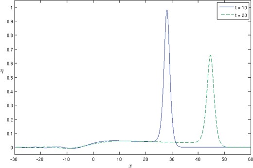
Figure 2:
Plot of |$ \eta(x,t) $| for |$ \epsilon=0.1 $| at times |$ t=10,20 $|, showing the decay in amplitude with increasing |$ t $| and the development of a decaying tail.
The asymptotic analysis presented in §3 relates to the solution of the perturbation equation (2.5a). While this is a linear equation for
|$ J(\theta,{\tilde{t}}) $|, a similar scheme to that described above is used. The presence of the
|$ (FJ)_{\theta} $| term requires two discrete Fourier transforms, akin to the treatment of the nonlinear term in the first scheme, with the other terms linear in
|$ J $| being removed using an integrating factor
|$ e^{h_{1}(k){\tilde{t}}} $|, where
|$ h_{1}(k)=-{i}k^{3}-4{i}k $|. The system to be solved is then
where
|$ F=\text{sech}^{2}\theta $| as before. Note that the final transform term is independent of
|$ {\tilde{t}} $| and hence is only evaluated once.
4.2. Numerical results for perturbation equation
We now consider numerical solutions of the perturbation equation (2.5a). In figure 3, numerical results for |$ J(\theta,{\tilde{t}}) $| are plotted for |$ {\tilde{t}}=2,5 $|. The first thing to note is that the core solution (the solution around |$ \theta=0 $|) has already approached a stationary form at |$ {\tilde{t}}=2 $|. Ahead of the core, the solution decreases rapidly to zero confirming the analysis presented in §3.2.1. Behind the core, a shelf of constant amplitude has appeared by |$ {\tilde{t}}=5 $| and the matching range between core and tail discussed in §3.2 corresponds to the region |$ -15 \lt\theta \lt -5 $|. Results for larger |$ {\tilde{t}} $| show that the extent of the shelf increases as |$ {\tilde{t}} $| increases.
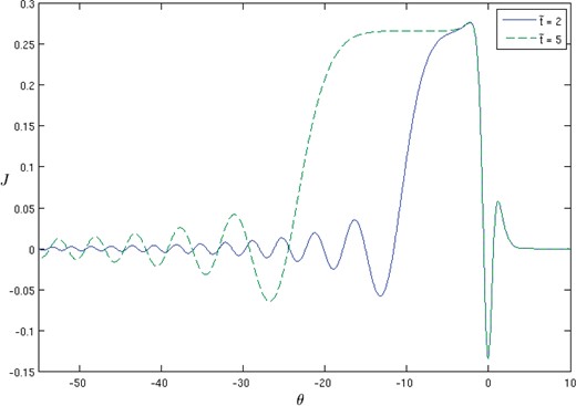
Figure 3:
Plot of numerical solution |$ J(\theta,{\tilde{t}}) $| for |$ {\tilde{t}}=2 $| and |$ {\tilde{t}}=5 $| illustrating the development of a stationary core about |$ \theta=0 $|, a constant ‘shelf’ behind the core, followed by an oscillating tail.
The stationary form of the solution around
|$ \theta=0 $| is now compared with the predicted analytic form of the core (3.6). Focussing first on the value of
|$ J(0,{\tilde{t}}) $|, the numerical results confirm the small
|$ {\tilde{t}} $| limit
|$ J(0,{\tilde{t}})\sim-\frac{14}{15}{\tilde{t}} $| from (3.2) and the large
|$ {\tilde{t}} $|-limit
|$ J(0,{\tilde{t}})\to-\frac{2}{15} $| from (3.6), with
|$ J(0,{\tilde{t}}) $| attaining 95% of its limiting value when
|$ {\tilde{t}}=0.7 $| and 99% by
|$ {\tilde{t}}=1.1 $|. The undetermined coefficient
|$ c $| appearing in the core solution can be directly extracted from the numerical results in a number of different ways. Directly from the numerical solution,
|$ J_{\theta}(0,t)\to c $| as
|$ t\to\infty $|. Alternatively, from the integral constraint (3.8b)
Here |$ \theta_{M} $| is taken to be in the overlap region, so |$ {\widehat{J}}\sim J $| in the integrand. The integral is evaluated using the numerical solution for |$ J $| and several values of |$ \theta_{M} $| were taken to ensure numerical consistency. A third method for calculating |$ c $|, comes by comparing the computed value of |$ J-{\widehat{J}}_{0} $| with |$ c\tanh\theta\text{sech}^{2}\theta $| at |$ \theta=\tanh^{-1}(1/\sqrt{3}) $|, the position of the maximum of |$ \tanh\theta\text{sech}^{2}\theta $|. At |$ {\tilde{t}}=5 $| all three methods give |$ c=0.0451 $| correct to 3 significant figures.
In figure 4 numerical results for |$ {\tilde{t}}=0.5,1,2 $| are compared with the analytic results using the computed value of |$ c $|. It is seen that there is good agreement between numerical and analytic solutions over the main part of the core, even for |$ {\tilde{t}}=0.5 $|. When |$ {\tilde{t}}=2 $|, results are indistinguishable over the range |$ -5 \lt\theta \lt 5 $|.

Figure 4:
Plot of numerical results for |$ J(\theta,{\tilde{t}}) $| for |$ {\tilde{t}}=0.5,1.0 $| and |$ 2.0 $| along with the analytic solution (3.6) with |$ c=0.0451 $| (symbols).
Looking now at the tail region, it was shown in §3.2.2 that the solution
|$ {\widetilde{J}} $| can be written in terms of a single universal function
|$ \phi(x) $|, The method used to extract this function from the numerical solution is to compare the derivative of the numerical solution and that of the analytic solution. From (3.10),
where
|$ z=(3{\tilde{t}})^{-\frac{1}{3}}(\theta+4{\tilde{t}}+1) $| from (3.13). Taking Fourier transforms with respect to
|$ z $| and using the convolution theorem then gives
since
|$ \mathcal{F}({\text{Ai}})=\exp(ik^{3}/3) $| . To obtain a numerical approximation of
|$ h $| (and hence
|$ \phi $|) we define
|$ Q(z,t) $| to be the computed value of
|$ J_{z} $| for
|$ \theta \lt\theta_{M} $| and zero elsewhere, with
|$ h(z,{\tilde{t}}) $| then given by
|$ \mathcal{F}^{-1}\left(\mathcal{F}(Q)/\exp(ik^{3}/3)\right) $| The exact value of the Fourier transform of the Airy function is used rather than the discrete transform over the finite range of the numerical calculation. This proves a better approach since the slow decay of
|$ {\text{Ai}}(z) $| accompanied by a shortening wavelength as
|$ z\to-\infty $|, leads to inaccuracy in the large wavenumber components of the discrete transform of the Airy function over a finite spatial range.
The function |$ \phi(x) $| extracted from the numerical solution at |$ {\tilde{t}}=5 $| is shown in figure 5. Extraction of |$ \phi(x) $| at |$ {\tilde{t}}=10 $| produced indistinguishable results, or equivalently, at |$ {\tilde{t}}=10 $| there is excellent agreement in the tail region between numerical results and (3.12) using the value of |$ \phi $| extracted at |$ {\tilde{t}}=5 $|. Thus the extracted value of |$ \phi $| can be used to give the solution in the tail region for all |$ {\tilde{t}} \gt 5 $|.
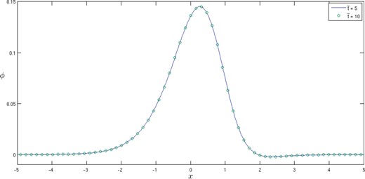
Figure 5:
Plot of |$ \phi(x) $| for |$ {\tilde{t}}=5 $| (line) and |$ {\tilde{t}}=10 $| (symbols), where |$ \phi(x)=h\left(x/(3{\tilde{t}}\right)^{\frac{1}{3}})/(3{\tilde{t}})^{\frac{1} {3}} $|, with |$ h $| extracted from the numerical solution of |$ J $| using (4.2).
Finally, the computed value of |$ \int_{-\infty}^{\infty}x^{2}\phi(x)dx=0.153 $| which using (3.14) gives a value of |$ c=0.0453 $|, agreeing to within |$ 0.5\% $| of the value extracted from the core solution.
4.3. Comparison of numerical results for BKdV and perturbation analysis
We now consider how the numerical solution of the full nonlinear equation (2.1) compares with the perturbation expansion. Considering the perturbation form given by (2.3), we define
where the
|$ N $| subscript denotes the numerical solution and
|$ \theta $| is given by (3.17). With
|$ \epsilon\ll 1 $|, and
|$ 1\ll t\ll\epsilon^{-1} $|,
|$ J_{N} $| should agree with the asymptotic result (3.12). For the core region where
|$ \theta=O(1) $|, in §4.2 it was seen that as
|$ t $| increases the asymptotic solution
|$ J $| approaches the stationary form
|$ {\widehat{J}} $|, with excellent agreement for
|$ {\tilde{t}} \gt 2 $|. In
figure 6,
|$ J_{N} $| is plotted as a function of
|$ \theta $| at
|$ t=1,2,4 $| for
|$ \epsilon=0.1 $| and
|$ 0.01 $|, and compared with the stationary core solution
|$ {\widehat{J}}(\theta) $|. It is seen that as
|$ \epsilon $| decreases, there is better agreement with
|$ {\widehat{J}} $|, but that as
|$ t $| increases the agreement with the stationary core solution worsens. This highlights the importance of the non-uniformity in the perturbation expansion as
|$ \tau=\epsilon t $| becomes
|$ O(1) $|.
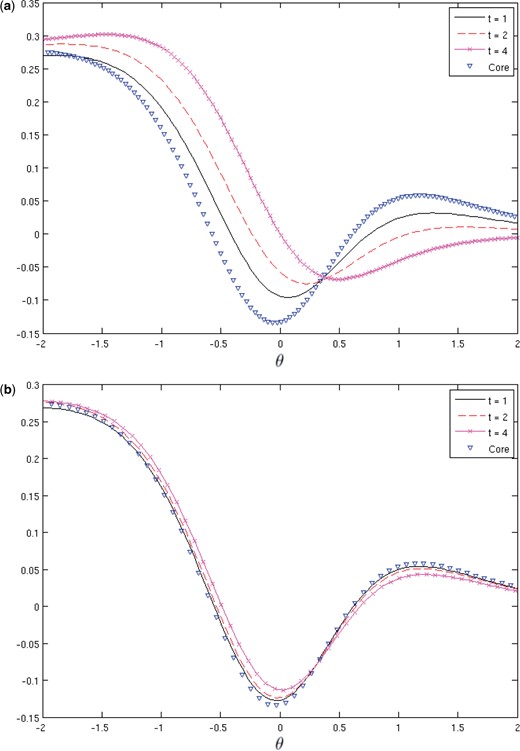
Figure 6:
Comparison of the computed value of |$ J_{N}(\theta,t) $| from (4.3) at times |$ t=1,2,4 $| (solid line, dashed line, line and symbols) for (a) |$ \epsilon=0.1 $| and (b) |$ \epsilon=0.01 $| with the steady core solution |$ {\widehat{J}}(\theta) $| (symbols) from (3.6) with |$ c=0.0451 $|.
The most direct check of the validity of the asymptotic predictions presented in §3 is by considering the maximum in the waveform and its location, and comparing numerical results with the asymptotic results summarised in §3.4. In
figure 7, the asymptotic prediction of the maximum amplitude of the disturbance is compared with the numerical results for
|$ \epsilon=0.1 $|. For
|$ t\ll 1 $|, there is good agreement with the small
|$ t $| prediction of (3.18a). For larger values of
|$ t $|, the numerical results are compared with the two asymptotic predictions
where
|$ \beta=\frac{16}{15}\epsilon t $| as previously defined.
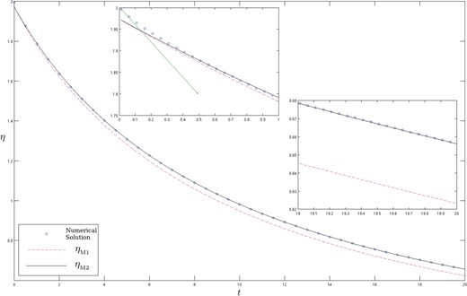
Figure 7:
Comparison of the maximum value of |$ \eta $| as a function of |$ t $| obtained numerically (solid line) for |$ \epsilon=0.1 $| and the asymptotic predictions |$ \eta_{M} $| and |$ \eta_{M1} $| given by (4.4). For small |$ t $| the asymptotic prediction (3.18a) is also plotted.
As noted earlier, the term |$ 2/(1+\beta) $| remains valid as a leading order approximation of the amplitude across the whole range of time studied, though the first correction term becomes comparable with the leading order term when |$ t=O(\epsilon^{-3}) $|, at which point the wave amplitude is |$ O(\epsilon^{2}) $|. Finally we validate the asymptotic prediction of the |$ x $|-position of the maximum. Rather than directly comparing |$ x_{M} $| obtained from the numerical solution with the asymptotic prediction (3.19c) valid when |$ t=O(\epsilon^{-1}) $|, to illustrate the accuracy of the perturbation analysis we choose to subtract off the leading order behaviour and hence in figure 8 we plot the numerical and asymptotic values of |$ x_{M}-4t $|, and excellent agreement is seen over a large time range.
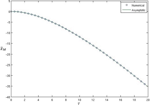
Figure 8:
Comparison of the position |$ {\widetilde{x}}_{M}=x_{M}(t)-4t $| of the maximum value of |$ \eta $| obtained numerically (symbols) for |$ \epsilon=0.1 $| and the asymptotic prediction (solid line) given by (3.19c).
5. Conclusions
The combination of asymptotic results and numerical results presented in §3 and §4 respectively provides the solution of the Burgers-Kortweg-de Vries (BKdV) equation upto |$ t\gg O(\epsilon^{-1}) $| by which time the solution is very small |$ O((\epsilon t)^{-1}) $|. We now compare the results of the current paper with earlier analysis of equations of the general form (1.3).
Asymptotic analysis of (1.3) began with [
7,
8] essentially following the method of §3.3, but focussing only on the leading order term for the amplitude variation over long timescales. Applying the solvability condition at leading order yields the result
The amplitude function arises as the solution of a first order ODE in the slow time
|$ \tau $| with its initial value fixed by the initial condition
|$ {\eta^{*}} $| at
|$ t=0 $|. While this analysis is not valid for
|$ t\ll 1 $|, at leading order the amplitude variation is correct. In [
8] results for the amplitude variation are presented for four different dissipation processes, including the case of magnetosonic waves being damped by electron-ion collisions which is described by the BKdV equation. Their results for this case agree with (3.18b) of the present analysis as
|$ \epsilon\to 0 $|. The analysis of Ott & Sudan was continued to higher order in [
13], again for the general case with dissipation
|$ \mathcal{R}(f) $|. Here the focus is on the higher order perturbation of the wave speed rather than the wave amplitude, though the amplitude can be readily deduced from this analysis. However when applying their general analysis to the BKdV equation an algebraic error is made. While their general result (2.20a) is valid, when this is applied to the specific case of BKdV their equation (3.8) should read
With this correction, the results agree with the present treatment, which has been validated by comparison with numerical results. However the key point to note is that the analysis of [13] does not fully determine the propagation speed as the initial value of |$ c_{1} $| remains undetermined. This has been calculated in the present paper.
We now turn our attention to the solutions of BKdV using inverse scattering, focussing in particular on the results of Karpman [
19]. The governing equation (5.1) of [
19] (which we denote as (K5.1)) is identical with (2.1) if
|$ u=-\eta $|,
|$ \kappa=\gamma $| and
|$ R(u)=u_{xx} $|. The unperturbed solution is
|$ u_{s}=-2\kappa^{2}\text{sech}^{2}{z} $| and so
|$ R[u_{s}]=-2\kappa^{4}(\text{sech}^{2}{z})_{zz} $|. Hence (K5.9) gives the variation of wavenumber as
which agrees with (3.7). Looking now at the amplitude of the shelf part of the tail,
|$ w_{s} $|, (K5.14) and (K5.45) gives
in agreement with the tail solution described in §3.2. Similarly the speed of propagation given by (K5.52)
agrees with the result obtained in §3.2.
Finally, looking at the expression for the core, (K5.53) should agree with the present analysis. However comparing (K5.53) with equation(3.1) of [
18] there is an inconsistency in the coefficient of
|$ p_{1}(z) $| in
|$ J(z,z^{\prime}) $|. After much algebraic manipulation, applying the result from [
18] to KdVB gives the same result as our result for
|$ J $| in (3.6) with
This agrees to three significant figures with the numerical value of |$ c $| obtained in §4.2. Thus the results of inverse scattering theory agree exactly with the |$ 1\ll t\ll\epsilon^{-1} $| asymptotic results of §3.2, at least for the core region, and indeed supplements the present analysis as |$ c $| is determined exactly. However identification of the breakdown of the solution as time increases from the inverse scattering analysis is unclear. In theory the exact structure of the tail should also be available from the inverse scattering analysis, though this is not discussed in [18, 19].
In summary the present paper has produced a description of the evolution of a weakly damped soliton governed by the Burgers-Kortweg-de Vries equation, covering three different time regimes, |$ t=o(1) $|, |$ t=O(1) $| and |$ t=O(\epsilon^{-1}) $|. Comparison is made with other analyses applicable to the different time regimes and all asymptotic results have been validated by careful comparison with numerical results. Of particular note is novel analysis of the tail region, leading to a description of the tail as a convolution of the Airy function and a characteristic function specific to the BKdV equation. The form of this function was extracted from the numerical solution, and while other forms of perturbed KdV will have different characteristic functions describing the tail region, exactly the same methods as described here can be used to determine this function.
References
[1]
Korteweg
D.J.
and
de Vries
F.
.
On the change of form of long waves advancing in a rectangular canal, and on a new type of long stationary waves
.
Philos. Mag
.,
39
:
422
–
443
,
1895
.
[2]
Hunter
J. K.
and
Vanden-Broeck
J. M.
.
Solitary and periodic gravity capillary waves of finite-amplitude
.
J. Fluid Mech
.,
134
:
205
–
219
,
1983
.
[3]
Hammerton
PW
and
Bassom
Andrew P
.
The effect of surface stress on interfacial solitary wave propagation
.
The Quarterly Journal of Mechanics and Applied Mathematics
,
66
(
3
):
395
–
416
,
2013
.
[4]
Easwaran
C. V.
.
Solitary waves on a conducting fluid layer
.
Phys. Fluids
,
31
(
11
):
3442
–
3443
,
1988
.
[5]
Papageorgiou
D. T.
,
Petropoulos
P. G.
and
Vanden-Broeck
J. M.
.
Gravity capillary waves in fluid layers under normal electric fields
.
Phys. Rev. E
,
72
(
5
):
051601
–1–3,
2005
.
[6]
Hammerton
P.W.
and
Bassom
A. P.
.
The effect of a normal electric field on wave propagation on a fluid film
.
Physics of Fluids
,
26
:
012107
,
2014
.
[7]
Ott
E
and
Sudan
RN
.
Nonlinear theory of ion acoustic waves with Landau damping
.
Physics of Fluids (1958-1988)
,
12
(
11
):
2388
–
2394
,
1969
.
[8]
Ott
E.
and
Sudan
R.N.
.
Damping of solitary waves
.
Phys. Fluids
,
13
:
1432
–
1434
,
1970
.
[9]
Keulegan
G. H.
.
Gradual damping of solitary waves
.
J. Research National Bureau Standards
,
40
(
6
):
487
–
498
,
1948
.
[10]
Johnson
RS
.
On an asymptotic solution of the Korteweg–de Vries equation with slowly varying coefficients
.
Journal of Fluid Mechanics
,
60
(
04
):
813
–
824
,
1973
.
[11]
Ko
K
and
Kuehl
HH
.
Korteweg-de Vries soliton in a slowly varying medium
.
Physical Review Letters
,
40
(
4
):
233
,
1978
.
[12]
Grimshaw
Roger
. Slowly varying solitary waves. i. Korteweg-de Vries equation. Proceedings of the Royal Society of London A: Mathematical, Physical and Engineering Sciences, 368(1734):359–375,
1979
.
[13]
Grimshaw
R
and
Mitsudera
H
.
Slowly varying solitary wave solutions of the perturbed Korteweg-de Vries equation revisited
.
Studies in Applied Mathematics
,
90
(
1
):
75
–
86
,
1993
.
[14]
Grimshaw
R.
,
Pelinovsky
E.
and
Talipova
T.
.
Damping of large-amplitude solitary waves
.
Wave Motion
,
37
(
4
):
351
–
364
,
2003
.
[15]
Ostrovsky
Lev
.
Asymptotic perturbation theory of waves
.
World Scientific
,
2014
.
[16]
Drazin
PG
and
Johnson
RS
.
Solitons: An Introduction
.
Cambridge University Press
,
1989
.
[17]
Karpman
VI
and
Maslov
EM
.
A perturbation theory for the Korteweg-de Vries equation
.
Physics Letters A
,
60
(
4
):
307
–
308
,
1977
.
[18]
Karpman
VI
and
Maslov
EM
.
Structure of tails produced under the action of perturbations on solitons
.
Soviet Journal of Experimental and Theoretical Physics
,
48
:
252
,
1978
.
[19]
Karpman
VI
.
Soliton evolution in the presence of perturbation
.
Physica Scripta
,
20
(
3-4
):
462
,
1979
.
[20]
Kaup
David J
and
Newell
Alan C
. Solitons as particles, oscillators, and in slowly changing media: a singular perturbation theory. Proceedings of the Royal Society of London A: Mathematical, Physical and Engineering Sciences, 361(1707):413–446,
1978
.
[21]
Knickerbocker
CJ
and
Newell
Alan C
.
Shelves and the Korteweg-de Vries equation
.
Journal of Fluid Mechanics
,
98
(
04
):
803
–
818
,
1980
.
[22]
Gao
Xin-Yi
.
Variety of the cosmic plasmas: general variable-coefficient Korteweg-de Vries-Burgers equation with experimental/observational support
.
EPL (Europhysics Letters)
,
110
(
1
):
15002
,
2015
.
[23]
Kuznetsov
VV
,
Nakoryakov
VE
,
Pokusaev
BG
and
Shreiber
IR
.
Propagation of perturbations in a gas-liquid mixture
.
Journal of Fluid Mechanics
,
85
(
1
):
85
–
96
,
1978
.
[24]
Harris
SE
and
Crighton
DG
.
Solitons, solitary waves, and voidage disturbances in gas-fluidized beds
.
Journal of Fluid Mechanics
,
266
:
243
–
276
,
1994
.
[25]
Fornberg
Bengt
.
A practical guide to pseudospectral methods
.
Cambridge University Press
,
1999
.
[26]
Trefethen
Lloyd N
.
Spectral methods in MATLAB
.
Siam
,
2000
.
[27]
Grundy
Dane
. The effect of surface stress on interfacial solitary waves. Phd thesis, University of East Anglia,
2019
.
[28]
Abramowitz
M.
and
Stegun
I. A.
.
Handbook of Mathematical Functions
.
Dover
,
1964
.
Appendices
Appendix A: Integral constraints on Perturbation Equation
In determining the solution of the linear perturbation equation, three integral constraints (3.2) are used. These constraints are derived in this appendix. For
|$ R(F) $| and
|$ L(J) $| defined by (2.4) and
|$ F=\text{sech}^{2}\theta $|, it can readily be shown that when
|$ J $| and its derivatives tend to zero as
|$ \theta\to\pm\infty $| then
Integrating (3.1) with respect to
|$ \theta $| and the product of (3.1) with
|$ F(\theta) $| then gives
Noting that
|$ J(\theta,0)=0 $| the first two integral constraints are obtained,
Integrating with respect to the transformed time variable |$ {\tilde{t}} $| then gives the final integral constraint required.
Appendix B: Useful Integral Results
In the main body of the paper, a number of integrals involving hyperbolic functions are used. All the integrals can be evaluated using standard techniques, their values are given together in this appendix for convenience. Using the shorthand notation
|$ T=\tanh\theta $| and
|$ S=\text{sech}\theta $|,
Appendix C: Convolution Integrals involving Airy functions
Defining the convolution
|$ R=f*{\text{Ai}} $| and
it is postulated that as long as
|$ f(x) $| decays sufficiently rapidly as
|$ |x|\to\infty $| so that
|$ C_{0}=\int_{-\infty}^{\infty}f(x)\ \gt dx $|,
|$ C_{1}=\int_{-\infty}^{\infty}xf(x)\ \gt dx $|,
|$ C_{2}=\int_{-\infty}^{\infty}x^{2}f(x)\ \gt dx $|, then
as
|$ z\to\infty $|. This corresponds to (3.11) with appropriate change of variables. Here it is verified that the result is true when
|$ f(x)=1 $| for
|$ a \lt x \lt b $| and zero elsewhere. Since all the results are linear in
|$ f(x) $|, this then validates the result for all piecewise constant functions with compact support.
We begin by defining the function
|$ I_{A}=\int_{-\infty}^{\infty}{\text{Ai}}(z^{\prime})\ \gt dz^{\prime} $| from which it follows that
Taking the limit as
|$ z\to\infty $|, and using the asymptotic forms [
28] for Airy functions gives
|$ I_{A}\sim 1 $|,
|$ q\sim z $|,
|$ r\sim{\textstyle{\frac{1}{2}}}z^{2} $| and
|$ s\sim{\textstyle\frac{1}{3}}(z^{3}+1) $|. Hence
Thus
|$ J\sim b-a $| and similarly, after some algebra,
Finally, substituting for
|$ f(x) $| in the expressions for
|$ C_{i} $|,
and the results (C.1) are validated.
© The Author(s) 2025. Published by Oxford University Press.
This is an Open Access article distributed under the terms of the Creative Commons Attribution License (
https://creativecommons.org/licenses/by/4.0/), which permits unrestricted reuse, distribution, and reproduction in any medium, provided the original work is properly cited.


