Summary
The boundary-value problem for the perturbation of an electric potential by a homogeneous anisotropic dielectric sphere in vacuum was formulated. The total potential in the exterior region was expanded in series of radial polynomials and tesseral harmonics, as is standard for the Laplace equation. A bijective transformation of space was carried out to formulate a series representation of the potential in the interior region. Boundary conditions on the spherical surface were enforced to derive a transition matrix that relates the expansion coefficients of the perturbation potential in the exterior region to those of the source potential. Far from the sphere, the perturbation potential decays as the inverse of the distance squared from the center of the sphere, as confirmed numerically when the source potential is due to either a point charge or a point dipole.
1. Introduction
When an object made of a certain linear homogeneous dielectric material is exposed to a time-invariant electric field, the atoms constituting the object interact with that electric field until an electrostatic steady state is reached a short time later (1, 2). This interaction is described in terms of the polarization which is the volumetric density of electric dipoles induced inside the object. The polarization is linearly proportional to the electric field , the proportionality constant being the dielectric susceptibility of the material multiplied by the free-space permittivity. Coulomb’s law then leads to the definition of the electric displacement field which is linearly related to by the permittivity of the material. The permittivity is scalar for isotropic materials but dyadic for anisotropic materials (3, 4).
Perturbation of an electrostatic field by a linear homogeneous dielectric object in free space has been studied for a long time (5–10), presently with biological (11), biomedical (12), electrochemical (13) and manufacturing (14) applications. Let us refer to the electric field present in the absence of the object as the source field, the difference between the electric field present at any location outside the object and the source electric field as the perturbation field, and the electric field present at any location inside the object as the internal field. The boundary-value problem for the electrostatic steady state is solved analytically by (i) expanding the source, perturbation and internal fields in terms of suitable basis functions and (ii) imposing appropriate boundary conditions at the surface of the perturbing object. The basis functions suitable for representing the source and the perturbation fields emerge from the eigenfunctions of the Laplace equation (5, 15, 16). When the object is made of an isotropic material, the basis functions suitable for representing the internal field also emerge from the eigenfunctions of the Laplace equation.
Our objective here is to show that analytic basis functions for representing the internal field are available when the perturbing object is composed of an anisotropic dielectric material (
17) described by the constitutive relation
where the permittivity dyadic
involves the diagonal dyadic
with
denoting the permittivity of free space. Any real symmetric dyadic can be written in the form of (
2) and (
3) by virtue of the principal axis theorem (
18, 19). The only conditions imposed by us are that the scalars
,
and
. Natural materials of such kind exist (
17). Materials of this kind can also be realized as homogenized composite materials by properly dispersing dielectric fibers in some host isotropic dielectric material (
20).
The positive definiteness (21) of allows for an affine transformation of space in which the governing equation from which the eigenfunctions are obtained is transformed into the Laplace equation. After solving the Laplace equation and obtaining the eigenfunctions in the transformed space, an inverse transformation of space is effected to obtain eigenfunctions in the original space for the material described by (1). We apply the procedure here to analytically investigate the perturbation of an electrostatic field by the anisotropic dielectric sphere.
The plan of this article is as follows. Section 2 contains the formulation of the boundary-value problem in terms of the electric potential. The expansion of the potential in the exterior region, which is vacuous, is presented in section 2.1; two illustrative examples of the source potential are provided in section 2.2; the expansion of the potential inside the anisotropic dielectric sphere is derived in section 2.3; boundary conditions are enforced in sections 2.4–2.6 to derive a transition matrix that relates the expansion coefficients of the perturbation potential to those of the source potential; the symmetries of the transition matrix are presented in section 2.7; and an asymptotic expression for the perturbation potential is derived in section 2.8. Section 3 presents illustrative numerical results. Conclusions are summarized in section 4.
2. Boundary-value problem
The region
is taken to be vacuous with constitutive relation
, whereas the spherical region
is occupied by the chosen material described by (
1). As electrostatic fields always satisfy the relation
(
2), it follows that
where
is the electric potential. Henceforth, we use the electric potential.
2.1 Potential in the region
The solution of the Laplace equation
in the spherical coordinate system
has been known for almost two centuries; thus (
2, 16),
where
is a normalization factor with
as the Kronecker delta and the tesseral harmonics
involve the associated Legendre function
(
22, 23). We have omitted the Condon–Shortley phase factor
in the definitions of both
and
(
24), because it is inessential. The coefficients
are associated with terms that are regular at the origin, whereas the coefficients
are associated with terms that are regular at infinity. The definitions of the tesseral harmonics mandate that
and
.
On the right side of (
5),
is the source potential whereas
is the perturbation potential. If the object were to be absent, (
5) would hold for all
with
.
2.2 Source potential
We proceed with the assumption that the coefficients are known but the coefficients are not. Furthermore, (8) is required to hold in some sufficiently large open region that contains the spherical region but not the region containing the source of .
Two illustrative examples of sources are a point charge
and a point dipole
. Suppose, first, that the source potential is due to a point charge
located at
with
; then
This potential can be expanded as (
2)
where the coefficients
and
Suppose, next, that the source potential is due to a point dipole of moment
located at
with
; then (
25)
where
denotes the gradient with respect to
. Equation (
11) still holds, but with
and
2.3 Potential in the region
Inside the dielectric sphere, the potential
does not obey the Laplace equation; instead,
In order to solve this equation, let us make an affine coordinate transformation:
where
and
The bijective transformation (16) maps a point on a spherical surface to a point on an ellipsoidal surface, since and , with lying in the same quadrant as and in the same quadrant as ; see Fig. 1.
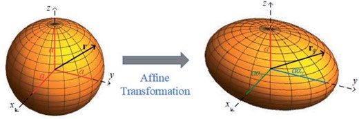
Fig. 1
Schematic depicting the mapping of a spherical surface into an ellipsoidal surface via (16).
Then, (
15) can be written as
that is,
which is the Laplace equation in the transformed space. Its solution is given by (
2, 16)
We must set
in order to exclude terms on the right side of (
20) that are not regular at the origin. Thereafter, on inverting the coordinate transformation, we obtain the internal potential
where
2.4 Boundary conditions
Since the tangential component of the electric field must be continuous across the interface
, and as there is no reason for the electric field to have an infinite magnitude anywhere on that interface, the potential must be continuous across that interface; hence,
Likewise, with the assumption of the interface
being charge-free, the normal component of the electric displacement must be continuous across that interface. Hence, by employing (
1), (
2) and (
4) for the displacement in the anisotropic region, we obtain
where
.
2.5 Transition matrix
After (i) substituting (
8), (
9) and (
21) in (
23), (ii) then multiplying both sides of the resulting equation by
and (iii) finally integrating over
and
, we get
where
and
Similarly, after (i) substituting (
8), (
9) and (
21) in (
24), (ii) then multiplying both sides of the resulting equation by
and (iii) finally integrating over
and
, we get
where
and
After truncating the indexes
and
so that only
and
are considered with
, (
25) and (
27) can be put together in matrix form symbolically as
and
where the matrixes
,
,
and
are diagonal matrixes. Since
to
are square matrixes, standard techniques can be used to solve (
29a) and (
29b) in order to determine the column vectors
and
in terms of
.
The perturbational characteristics of the anisotropic dielectric sphere are encapsulated in the transition matrix
that relates the column vectors
and
via
where
The transition matrix is a diagonal matrix when the sphere is made of an isotropic dielectric material (that is, , where is the identity dyadic) because is then a diagonal matrix. In general, is not a diagonal matrix when the sphere is made of an anisotropic dielectric material, so that is not a diagonal matrix either.
2.6 Reduction of computational effort
Computational effort for the integrals (
26c) and (
28c) can be significantly reduced on noting that
furthermore,
lies in the same quadrant as
and
in the same
quadrant as
. Therefore,
and
can be used instead of (
26c) and (
28c), respectively.
2.7 Symmetries of the transition matrix
By virtue of its definition through (30), the transition matrix does not depend on the source potential. This matrix depends only on the radius and the constitutive parameters , and of the perturbing sphere.
Let us denote each element of the transition matrix defined in (31) by . It was verified numerically that if the following three conditions are satisfied:
- (i)
,
- (ii)
and have the same parity (that is, even or odd), and
- (iii)
and have the same parity.
Finally, let the transition matrix elements be denoted as for a specific choice of the anisotropy parameters, but as after and have been interchanged without changing . In other words, changes to when the sphere is rotated about the axis by . Then, the following relationships exist between the pre- and post-rotation transition matrixes:
2.8 Asymptotic expression for perturbation potential
Equation (
9) can be written as
Since
emerges from calculations for a sphere whether
or not, the asymptotic behavior of the perturbation potential far away from the sphere is given by
where the asymptotic perturbation
Accordingly, the first term on the right side of (37) does not exist in the equatorial plane (i.e., ) whereas the second term is absent on the axis (that is ).
Now, the perturbation potential must depend on the source as well as on the radius of the sphere. For the two sources chosen for illustrative results, must depend linearly on both the sign and the magnitude of or (as appropriate). The location of either of the two sources enters the potential expressions only by means of the source-potential coefficients , which are proportional to for the point charge and to for the point dipole, according to (12b) and (14b). Since the transition matrix does not depend on the source, the perturbation-potential coefficients , and increase/decrease as decreases/increases. Accordingly, the magnitude of increases/decreases as decreases/increases.
Since the coefficients
cannot depend on
, it follows then from (
25) and (
27) that
Dimensional analysis of (
5) also supports this proportionality. Equations (
37) and (
39) then yield accordingly,
3. Numerical results and discussion
3.1 Preliminaries
For all numerical results presented in this section, we fixed
and
.
Note that
when the sphere is made of an isotropic material (that is,
).
A Mathematica™ program was written to calculate the normalized functions
and
where the normalized radius
and
is some reference value of the source potential. The reference value can be chosen as
. This choice works well if the source is an external point charge and also if the source is an external point dipole except when
. By virtue of its definition and the dependencies of
discussed in section
2.8,
- (i)
is independent of or (as appropriate),
- (ii)
increases/decreases as decreases/increases, and
- (iii)
is directly proportional to .
A convergence test was carried out with respect to
, by calculating the integral
at diverse values of
as
was incremented by unity. The iterative process of increasing
was terminated when
within a preset tolerance of
. The adequate value of
was higher for lower
, with
sufficient for
.
The theory described in section 2 was validated by comparing its results for the perturbation of the source potential by an isotropic dielectric sphere with the corresponding exact solutions available in the literature. First, the source was taken to be a point charge located on the axis (i.e., ) at ; note that is irrelevant when . Excellent agreement was obtained with respect to the exact solution (26) for all examined values of and . Next, the point charge was replaced by a point dipole. Again, excellent agreement was found with respect to the corresponding exact solutions (25, 27).
3.2 Normalized asymptotic perturbation
Having clarified in section 3.1 the effects of the parameters , , , and on the normalized asymptotic perturbation , we present numerical results for the variations of as a function of the sphere’s anisotropy parameters and for the following three cases:
Case 1: ,
Case 2: , and
Case 3: .
Plots of the perturbation-potential coefficients , and as functions of and are examined in conjunction with the corresponding plots of versus and for cm, , and . All calculations were made for either a point charge of magnitude C or a point dipole of moment C m.
3.2.1 Case 1 (, )
We varied but kept fixed. Figure 2 shows plots of , and versus for a point-charge source as well as for a point-dipole source with . Angular profiles of for the same sources are depicted in Fig. 3 for , and in Fig. 4 for .
![${\cal B}_{\rm e01}$, ${\cal B}_{\rm e11}$ and ${\cal B}_{\rm o11}$ versus $\bar{\alpha} \in [0.5,1.5]$ when $\alpha_{\rm x}=\bar{\alpha}$, $\alpha_{\rm y}=1$, and the source is either (a) a point charge or (b-d) a point dipole with (b) $\hat{{\bf p}} = \hat{{\bf x}}$, (c) $\hat{{\bf p}} = \hat{{\bf y}}$ and (d) $\hat{{\bf p}} = \hat{{\bf z}}$, respectively.](https://oup.silverchair-cdn.com/oup/backfile/Content_public/Journal/qjmam/74/4/10.1093_qjmam_hbab013/3/m_hbab013f2.jpeg?Expires=1750217724&Signature=DIU4CBP0KxJH9k6e0wTXJubrTtD5bZiO5rrUFsEJSU9tXsnXgq4strjqSULTu5hIJZT7OXRW4o-hZXETw7uojb6udv71U36xxGZLKnnqKU6GZWXS0TZqDTOgqOwFLBRsqIk2X0OHcS5RitMeDDnK05WeQajrIiOhFr1SqJ8QChqHPZ7f1iaCrpV4n5FQ7JBjpv--3CsJbiC1qRbTkCMezzhxR5tq7qLJbT0H7dX4SblASghiYBgI5cfBYL8wxiZ0oqELTFvZo9P8c9D~LzlDxhN17Q4mHkZ71Huz3LUIzHZWcJT1xtQUERztt5hGeK6YYDMTnFSrM~N4D94-EbjwyQ__&Key-Pair-Id=APKAIE5G5CRDK6RD3PGA)
Fig. 2
, and versus when , , and the source is either (a) a point charge or (b-d) a point dipole with (b) , (c) and (d) , respectively.
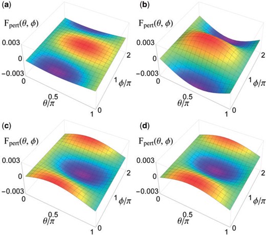
Fig. 3
versus and when , , and the source is either (a) a point charge or (b-d) a point dipole with (b) , (c) and (d) , respectively.
For a point-charge source, decreases with in Fig. 2(a). Thus, decreases but increases as changes from to , as can be gathered from Figs. 3(a) and 4(a). Also, increases and decreases with increasing . Therefore, increases but decreases as changes from to .
Next, for the point-dipole sources, increases with increasing for all three dipole orientations, as is clear from Figs. 2(b)–(d); the largest increase is observed for . Hence, a comparison of Figs. 3(b)–(d) and 4(b)–(d) reveals that increases but decreases as changes from to . The rate of these increases or decreases is highest for , moderate for , and lowest for .
Besides, for , both and increase with in Fig. 2(b) and, thus, and also increase with in Figs. 3(b) and 4(b). On the other hand, for and , decreases in Fig. 2(c) but increases in Fig. 2(d) as increases. Therefore, decreases and increases with , as can be gathered from comparing Figs. 3(c) and (d) with Figs. 4(c) and (d), respectively.
3.2.2 Case 2 (, )
Next, we fixed but varied . The dependencies of the coefficients , , and on are depicted in Fig. 5, whereas the angular profiles of are depicted in Fig. 6 for and Fig. 7 for .
![${\cal B}_{\rm e01}$, ${\cal B}_{\rm e11}$ and ${\cal B}_{\rm o11}$ versus $\bar{\alpha} \in [0.5,1.5]$ when $\alpha_{\rm x}=1$, $\alpha_{\rm y}=\bar{\alpha}$, and the source is either (a) a point charge or (b–d) a point dipole with (b) $\hat{{\bf p}} = \hat{{\bf x}}$, (c) $\hat{{\bf p}} = \hat{{\bf y}}$ and (d) $\hat{{\bf p}} = \hat{{\bf z}}$, respectively.](https://oup.silverchair-cdn.com/oup/backfile/Content_public/Journal/qjmam/74/4/10.1093_qjmam_hbab013/3/m_hbab013f5.jpeg?Expires=1750217724&Signature=yXGjdRrxpBV6LRYbah~XP65xxx6G~rkO9KeMTs8sN8e8y1ci4YgF9KunsVIhc-ZiQzXqPXCEjsFSEJJ0OW7VL~-PfSpzxDg23vq0Kb5awhupNpc~Brk4-7DHxshNYMb4MqmV4Ny5QPbIFIBmLyIl6535BYpg~bq6rDkFVxa6lYKnzMVkSBxCtheC29poNxfFyC9~JYzxnmZG3Ohd5rFGa4GkrLfd8B4iB3i167KvOJEIfOM7fGJ6H06ZcBlWuH-4cmu8TsbkU0BMXRksug2kyrua0ci5o9bOIXiNO2Un8Kk83WahIQdXY77QcPg6X6mGlEEzJx0QzwbQUZQWDsz61w__&Key-Pair-Id=APKAIE5G5CRDK6RD3PGA)
Fig. 5
, and versus when , , and the source is either (a) a point charge or (b–d) a point dipole with (b) , (c) and (d) , respectively.

Fig. 6
As in Fig. 3, except for and .
For all four types of source considered, varies with in Case 1 in the same way as it varies with in Case 2. Hence, the characteristics of and in Case 2 replicate those in Case 1. Also, if or is an increasing (decreasing) function of in Case 1, then it is a decreasing (increasing) function of in Case 2. Therefore, the characteristics of and in Case 2 are opposed to those in Case 1.
3.2.3 Case 3 ()
Finally, we set . The corresponding plots for vs are depicted in Fig. 8, and for versus and are depicted in Fig. 9 for , and in Fig. 10 for .
The curves of versus have the same increasing/decreasing tendencies with the respective ones in Cases 1 and 2; however, the values of and the rate of increase/decrease w.r.t. are definitely different. Furthermore, in Case 3, the increasing/decreasing tendencies of and with are as those in Cases 1 and 2, respectively.
3.3 Normalized perturbation potential
Unlike
, the normalized perturbation potential
depends additionally on the distance
from the origin to the observation point. With the same values of
,
,
,
,
and
as in section
3.2, we also examined the perturbation potential’s variations with respect to
, with
and
fixed, for a point-charge source as well as for a point-dipole source with
.
Figure 11 presents the angular profiles of
,
Fig. 12 of
, and
Fig. 13 of
, where
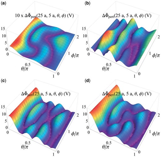
Fig. 11
versus and when , , and the source is either (a) a point charge or (b-d) a point dipole with (b) , (c) and (d) , respectively.
For all four sources, the inequalities
hold true. This indicates that, as
increases,
decreases as expected in every direction (indicated by
). Also, the surface of
is smoother and less undulating than the surface of
, which is smoother and flatter than the surface of
. This is due to the waning of the higher-order terms on the right side of (
35) as
increases. These higher-order terms have a strong effect on
at observation points close to the sphere, the strongest such effects being observed for the dipole sources, as is evident from
Figs. 11(b)–(d). Indeed, the decrease of
and the smoothening of its angular profile with increase of
is reflected in the limit
Finally, on comparing Figs. 11–13, we observe that the portions of the - plane corresponding to the maximum/minimum increase in remain almost the same as increases, for each of the four source potentials considered.
4. Concluding remarks
We formulated and solved the boundary-value problem for the perturbation of an electric potential by a homogeneous anisotropic dielectric sphere in vacuum. As is commonplace for the exterior region, the source potential and the perturbation potential were represented in terms of the standard solutions of the Laplace equation in the spherical coordinate system. A bijective spatial transformation was implemented for the interior region in order to formulate the series representation of the internal potential. Boundary conditions on the spherical surface were enforced and then the orthogonality of tesseral harmonics was employed to derive a transition matrix that relates the expansion coefficients of the perturbation potential in the exterior region to those of the source potential. The angular profile of the perturbation profile changes with distance from the center of the sphere, but eventually it settles down with the perturbation potential decaying as the inverse of the distance squared from the center of the sphere.
Acknowledgement
A. Lakhtakia is grateful to the Charles Godfrey Binder Endowment at Penn State for ongoing support of his research activities.
References
1.
Smythe
W. R.
,
Static and Dynamic Electricity
, 2nd edn. (
McGraw–Hill
,
New York, NY, USA
1950
).
2.
Jackson
J. D.
,
Classical Electrodynamics
, 3rd edn.. (
Wiley
,
Hoboken, NJ, USA
1999
).
3.
Gersten
J. I.
and
Smith
F. W.
,
The Physics and Chemistry of Materials
(
Wiley
,
New York, NY, USA
2001
).
4.
Nye
J. F.
,
Physical Properties of Crystals: Their Representation by Tensors and Matrices
(
Oxford University Press
,
Oxford, UK
1985
).
5.
Kellogg
O. D.
,
Foundations of Potential Theory
(
Dover
,
New York, NY, USA
1953
).
6.
Williams
W. E.
,
Some boundary value problems in potential theory
,
Q. J. Mech. Appl. Math.
14
(
1961
)
443
–
452
.
7.
Love
J. D.
,
Dielectric sphere-sphere and sphere-plane problems in electrostatics
,
Q. J. Mech. Appl. Math.
28
(
1975
)
449
–
471
.
8.
Jones
D. S.
, The scattering of long electromagnetic waves,
Q. J. Mech. Appl. Math.
33
(
1980
)
105
–
122
.
9.
Lindell
I. V.
,
Electrostatic image theory for the dielectric sphere
,
Radio Sci.
27
(
1992
)
1
–
8
.
10.
Majić,
M. R. A
Auguié
B.
and
Le Ru,
E. C.
Laplace’s equation for a point source near a sphere: improved internal solution using spheroidal harmonics
,
IMA J. Appl. Math.
83
(
2018
)
895
–
907
.
11.
Sukhorukov
V. L.
,
Meedt,
G.
Kürschner
M.
and
Zimmermann,
U.
A single-shell model for biological cells extended to account for the dielectric anisotropy of the plasma membrane
,
J. Electrostat.
50
(
2001
)
191
–
204
.
12.
Woeppel
K.
,
Yanga
Q.
and
Cui
X. T.
,
Recent advances in neural electrode–tissue interfaces
,
Curr. Opin. Biomed. Eng.
4
(
2017
)
21
–
31
.
13.
Everts
J. C.
,
Senyuk
B.
,
Mundoor
H.
,
Ravnik
M.
and
Smalyukh
I. I.
,
Anisotropic electrostatic screening of charged colloids in nematic solvents
,
Sci. Adv.
7
(
2021
)
eabd0662
.
14.
Plog
J.
,
Jiang
Y.
,
Pan
Y.
and
Yarin
A. L.
,
Electrostatic charging and deflection of droplets for drop-on-demand 3D printing within confinements
,
Addit. Manufact.
36
(
2020
)
101400
.
15.
Medková,
D.
The Laplace Equation: Boundary Value Problems on Bounded and Unbounded Lipschitz Domains
(
Springer, Cham
,
Switzerland
2018
).
16.
Moon
P.
and
Spencer
D. E.
,
Field Theory Handbook: Including Coordinate Systems, Differential Equations and Their Solutions
, 2nd edn. (
Springer, Berlin
,
Germany
1971
).
17.
Auld
B. A.
,
Acoustic Fields and Waves in Solids
, Vol.
I
, 2nd edn. (
Krieger, Malabar, FL
,
USA
1990
).
18.
Charnow
A.
and
Charnow
E.
,
Fields for which the principal axis theorem is valid
,
Math. Mag.
59
(
1986
)
222
–
225
.
19.
Strang
G.
,
Introduction to Linear Algebra
, 5th edn. (
Wellesley–Cambridge
,
Wellesley, MA, USA
2016
).
20.
Mackay
T. G.
and
Lakhtakia
A.
,
Modern Analytical Electromagnetic Homogenization with Mathematica®
, 2nd edn. (
IoP
,
Bristol, UK
2020
).
21.
Lütkepohl,
H.
Handbook of Matrices
(
Wiley, Chichester
,
West Sussex, UK
1996
).
22.
Morse
P. M.
and
Feshbach
H.
,
Methods of Theoretical Physics
, Vol.
II
(
McGraw–Hill
,
New York, NY, USA
1953
) .
23.
Alkhoori
H. M.
,
Lakhtakia
A.
,
Breakall
J. K.
and
Bohren
C. F.
,
Plane-wave scattering by an ellipsoid composed of an orthorhombic dielectric–magnetic material
,
J. Optic. Soc. Am. A
35
(
2018
)
1549
–
1559
.
24.
Suta
M.
,
Cimpoesu
F.
and
Urland
W.
,
The angular overlap model of ligand field theory for elements: An intuitive approach building bridges between theory and experiment
,
Coord. Chem. Rev.
441
(
2021
)
231981
.
25.
Tsitsas
N. L.
and
Martin
P. A.
,
Finding a source inside a sphere
,
Inverse Problems
28
(
2012
)
015003
.
26.
Stratton
J. A.
,
Electromagnetic Theory
(
McGraw–Hill
,
New York, NY, USA
1941
).
27.
Zurita-Sánchez,
J. R.
Quasi-static electromagnetic fields created by an electric dipole in the vicinity of a dielectric sphere: method of images
,
Revista Mexicana de Física
55
(
2009
)
443
–
449
.
28.
Van Bladel
J.
,
Electromagnetic Fields
, 2nd edn. (
Wiley-IEEE Press
,
Piscataway, NJ, USA
2007
).
Appendix
Equation (
15) transforms into (
18) as follows. By virtue of (A4.57) of Ref. ((
28)), we have
because
is both symmetric and independent of
. Setting
in (
A.1), we get
Now, the transformation (
16) delivers
so that
follows from (
A.2). By means of (
16), the right side of (
A.3) simplifies to yield
Equation (A4.57) of Ref. ((
28)) also delivers
Equation (18) follows from (A.4) and (A.5).
© The Author, 2021. Published by Oxford University Press.
This is an Open Access article distributed under the terms of the Creative Commons Attribution License (
https://creativecommons.org/licenses/by/4.0/), which permits unrestricted reuse, distribution, and reproduction in any medium, provided the original work is properly cited.


