Capillary-gravity waves on the interface of two dielectric fluid layers under normal electric fields

Doak, A; Gao, T; Vanden-Broeck, J -M; Kandola, J J S

doi:10.1093/qjmam/hbaa009

Summary

In this article, we consider capillary-gravity waves propagating on the interface of two dielectric fluids under the influence of normal electric fields. The density of the upper fluid is assumed to be much smaller than the lower one. Linear and weakly nonlinear theories are studied. The connection to the results in other limit configurations is discussed. Fully nonlinear computations for travelling wave solutions are achieved via a boundary integral equation method. Periodic waves, solitary waves and generalised solitary waves are presented. The bifurcation of generalised solitary waves is discussed in detail.

Issue Section:

Articles

1. Introduction

Electrohydrodynamics (EHD) is concerned with the interaction of charged fluid motion with electric fields. When performing experiments, it is much easier to artificially manipulate the electric field than it is to vary surface tension. EHD has numerous industrial chemical engineering applications, such as electrospray technology (1–3), enhanced heat transfer (4), cooling systems which make use of conducting fluids in high-power devices (5), coating processes (6, 7) and so on. Two comprehensive reviews of advances and applications in EHD can be found in (8, 9). EHD problems often concern an interface between two fluids, and hence an enhancement in the understanding of fluid dynamics benefits the engineering community. Research on EHD interfacial waves was first conducted by (10), who showed theoretically and experimentally that the interface between a dielectric and a conducting fluid can be destabilised by normal electric fields. It was followed by (11), who performed a linear stability analysis of interfacial flows under electric fields that are parallel to the undisturbed surface, and found that short waves can be regularised under such circumstances. Being inspired by these two earlier works, many authors considered the role of EHD in both stabilising and destabilising interfacial fluid configurations. Kelvin–Helmholtz and Rayleigh–Taylor instability were considered by (12) and (13, 14) respectively, where horizontal electric fields were shown to be capable of suppressing these instabilities. The results were achieved by using reduced model equations in (12, 13) and by direct numerical simulations in (14). Travelling waves of finite amplitude on capillary sheets under the influence of tangential electric fields were computed in (15) by a boundary integral equation method.

The problem of capillary-gravity travelling waves propagating under vertical electric fields in two-dimensions has been investigated by many authors for different configurations as summarised by (9). The general set up consists of two immiscible dielectric fluids with different electric permittivities, with an interface in between. To reduce the complexity of the problem, some assumptions were made in previous works. For example, (16, 17) assumed that the upper layer is much larger than the lower one. Under the long wave limits, Boussinesq-type models were derived and computed in the former literature whereas a boundary integral equation method was used to compute fully nonlinear solutions in the latter one. Another common assumption is to consider the case when one of the layers is a perfect conductor. Korteweg de-Vries (KdV), modified KdV, forced KdV and KdV-Benjamin–Ono equations were derived for long waves respectively by (18–20, 22) in the case of a layer of conducting fluid on the bottom and a dielectric on the top. The works were extended to three dimensions by (23, 24). On the other hand, in the case where the upper region is a conducting gas, (25, 26) computed fully nonlinear travelling solitary waves on a dielectric fluid of infinite and finite depth respectively as well as their dynamics based on a time-dependent hodograph transformation technique. To our knowledge, no fully nonlinear computations have been performed so far for the general set up of two dielectrics with two finite depth layers. This is the main focus of this work.

The rest of the article is structured as follows. Detailed formulations are given in section 2, and followed by a linear theory in section 3 and a weakly nonlinear theory in section 4. The numerical scheme and the results are presented respectively in section 5 and 6. A conclusion is given in section 7.

2. Formulation

We consider the two-dimensional irrotational flow of an inviscid incompressible fluid of finite depth that is bounded below by an electrode and above by a hydrodynamically passive gas, which in turn is bounded above by another electrode (see Fig. 1). The fluid and the passive gas are assumed to be perfect dielectrics with permittivity $ϵ_{1}$ and $ϵ_{2},$ respectively. The problem can be formulated by using Cartesian coordinates with the $y$ -axis directed vertically upwards and $y = 0$ at the mean level of the interface between the fluid and the gas. We take $h$ as the undisturbed depth of the fluid, and $h^{+}$ as the undisturbed depth of the passive gas. The effects of gravity $g$ and the surface tension $σ$ are both included in the formulation. The interface between the fluid and the gas is a free surface whose unknown equation is denoted by $y = ζ (x, t)$ ⁠. A wavetrain is assumed to travel rightwards following the direction of the $x$ -axis. We denote the voltage potential in the fluid and the gas by $v$ and $w,$ respectively. Without loss of generality, we choose $v = 0$ on the bottom electrode. Continuity of the tangential component of the electric fields results in the condition that $v$ and $w$ are equal on the free-surface, up to an arbitrary constant, which without loss of generality we take to be zero. The potential on the upper electrode $w$ is then a fixed parameter of the problem, which we denote by $w = E_{0} h^{+}$ ⁠. This choice of $w$ on the upper electrode is chosen such that, in the case where $h^{+} \to \infty$ ⁠, the electric field approaches a uniform vertical electric field with strength $E_{0}$ ⁠.

$Configuration of the problem. The gravity acts in the negative $y$-direction. We denote the equation of the unknown free surface by $y=\zeta(x,t)$.$

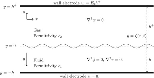
Fig. 1

Configuration of the problem. The gravity acts in the negative $y$ -direction. We denote the equation of the unknown free surface by $y = ζ (x, t)$ ⁠.

Open in new tab Download slide

Since the fluid motion can be described by a velocity potential function

ϕ (x, y, t)

⁠,the governing equations can then be written as

\begin{aligned} \nabla^{2} ϕ = 0, & for - h < y < ζ (x, t), \end{aligned}

(2.1)

\begin{aligned} \nabla^{2} v = 0, & for - h < y < ζ (x, t), \end{aligned}

(2.2)

\begin{aligned} \nabla^{2} w = 0, & for ζ (x, t) < y < h^{+}, \end{aligned}

(2.3)

\begin{aligned} ζ_{t} = ϕ_{y} - ϕ_{x} ζ_{x}, & on y = ζ (x, t), \end{aligned}

(2.4)

\begin{aligned} ϕ_{y} = 0, & on y = - h . \end{aligned}

(2.5)

\begin{aligned} w = E_{0} h^{+}, & on y = h^{+}, \end{aligned}

(2.6)

\begin{aligned} v = 0 & on y = - h, \end{aligned}

(2.7)

\begin{aligned} v_{x} + ζ_{x} v_{y} = w_{x} + ζ_{x} w_{y} & on y = ζ (x, t), \end{aligned}

(2.8)

\begin{aligned} v_{y} - ζ_{x} v_{x} = Λ (w_{y} - ζ_{x} w_{x}) & on y = ζ (x, t), \end{aligned}

(2.9)

and

ϕ_{t} + \frac{1}{2} | \nabla ϕ |^{2} + g ζ - \frac{T}{ρ} \frac{ζ_{x x}}{(1 + ζ_{x}^{2})^{3 / 2}} + σ_{e} = B, on y = ζ (x, t),

(2.10)

where the subscripts denote partial derivatives,

B

is the Bernoulli constant and

σ_{e}

is the Maxwell stress given by

\begin{array}{r} σ_{e} = - \frac{ϵ_{1}}{ρ (1 + ζ_{x}^{2})} [\frac{1}{2} (1 - ζ_{x}^{2}) (v_{x}^{2} - v_{y}^{2} - Λ (w_{x}^{2} - w_{y}^{2})) + 2 ζ_{x} (v_{x} v_{y} - Λ w_{x} w_{y})] \end{array}

(2.11)

with

Λ = ϵ_{2} / ϵ_{1}

being the ratio of the permittivity from two layers. The last three terms of (2.10) are the forces due to gravity, surface tension, and the Maxwell stresses due to the electric field. Equations (2.4) and (2.5) are the kinematic boundary conditions on the interface and bottom electrode respectively. The conditions (2.6) and (2.7) fix the electric potentials at the electrodes. Finally, continuity of the tangential components of the electric field and continuity of the normal component of the displacement field are given by (2.8) and (2.9) respectively. By making use of (2.8), (2.9), the Maxwell stress (2.11) can be simplified as

\begin{array}{r} σ_{e} = \frac{ϵ_{1} (Λ - 1)}{2 ρ Λ (1 + ζ_{x}^{2})} [(Λ + ζ_{x}^{2}) v_{x}^{2} + (Λ ζ_{x}^{2} + 1) v_{y}^{2} + 2 (Λ - 1) v_{x} v_{y} ζ_{x}] . \end{array}

(2.12)

3. Linear theory

By choosing

h

⁠,

\sqrt{h / g}

and

E_{0}

as the reference length, time and the strength of electric field, the bottom is at the level

y = - 1

⁠, and the system is still governed by the Laplace equations but with the dynamic boundary condition (2.10) becoming

\begin{array}{r} ϕ_{t} + \frac{1}{2} | \nabla ϕ |^{2} + ζ + σ_{e} - τ \frac{ζ_{x x}}{(1 + ζ_{x}^{2})^{3 / 2}} = B on y = ζ (x, t), \end{array}

(3.1)

and

\begin{array}{r} σ_{e} = \frac{E_{b} (Λ - 1)}{2 Λ (1 + ζ_{x}^{2})} [(Λ + ζ_{x}^{2}) v_{x}^{2} + (Λ ζ_{x}^{2} + 1) v_{y}^{2} + 2 (Λ - 1) v_{x} v_{y} ζ_{x}], \end{array}

(3.2)

where

τ

is the inverse Bond number and

E_{b}

is the inverse electric Bond number defined by

\begin{array}{r} τ = \frac{T}{ρ g h^{2}}, E_{b} = \frac{ϵ_{1} E_{0}^{2}}{ρ g h} . \end{array}

(3.3)

The boundary conditions on the voltage potential are now scaled to be

\begin{aligned} v = 0, on y = - 1, \end{aligned}

(3.4)

\begin{aligned} w = R, on y = R, \end{aligned}

(3.5)

where

R = h^{+} / h

⁠. The kinematic conditions (2.4), (2.5), (2.8) and (2.9) remain unchanged. The trivial solution

ζ (x, t) = 0

⁠,

ϕ (x, y, t) = 0

gives rise to the following electric potentials

\begin{array}{rcl} v = P Λ (y + 1), \end{array}

(3.6)

\begin{array}{rcl} w = P (y - R) + R, \end{array}

(3.7)

where

P = R / (R + Λ)

⁠. We linearise the system about the trivial solution by writing

\begin{array}{rcl} ζ (x, t) = ℜ {A ϵ e^{i (k x - ω t)}}, \end{array}

(3.8)

\begin{array}{rcl} ϕ (x, y, t) = ℜ {B ϵ e^{i (k x - ω t)} \cosh k (y + 1)}, \end{array}

(3.9)

\begin{array}{rcl} v (x, y, t) = P Λ (y + 1) + ℜ {C ϵ e^{i (k x - ω t)} \sinh k (y + 1)}, \end{array}

(3.10)

\begin{array}{rcl} w (x, y, t) = P (y - R) + R + ℜ {D ϵ e^{i (k x - ω t)} \sinh k (y - R)}, \end{array}

(3.11)

where

| ϵ | ≪ 1

⁠,

ω

is the angular frequency,

k

is the wavenumber,

ℜ

represents the real part, and

A

⁠,

B,

C

and

D

are constants to be found. For right-travelling waves, the wavenumber

k

is always positive. The forms of these solutions ensure that (2.1), (2.2), (2.3), (2.5), (3.5) and (3.4) are satisfied. Substituting into (2.4) and (2.10) yields the following dispersion relation

\begin{array}{r} c^{2} = (\frac{1}{k} + τ k) \tanh k - E_{b} \frac{P^{2} {(1 - Λ)}^{2} \tanh (k)}{\tanh (k) + Λ^{- 1} \tanh (k R)} . \end{array}

(3.12)

Here, $c = ω / k$ is the wave phase speed. It can be seen from equation (3.8) that if $c^{2} < 0$ for some $k > 0$ ⁠, then the configuration is linearly unstable to perturbations with wavenumber $k$ ⁠. Noting that the term following $E_{b}$ is positive for all $k > 0$ ⁠, we can see that the vertical electric field is destabilising when the top electrode is held to a higher electric potential than the bottom one, while the effects of surface tension are stabilising. There are a variety of limiting configurations we will consider below.

The dispersion relation (3.12) for a variety of parameters is shown in Fig. 2.

In the case where the upper electrode is placed infinitely far away from the fluid (⁠ $R \to \infty$ ⁠), we find that
$\begin{array}{r} c_{1}^{2} = (\frac{1}{k} + τ k) \tanh k - E_{b} \frac{{(1 - Λ)}^{2}}{1 + Λ^{- 1} \coth (k)}, \end{array}$
(3.13)
This configuration was seen in (16, 17), where the electric field at $y \to \infty$ is given by $w = E_{0} y$ ⁠.
In the particular case where the gas is a perfect conductor, as explored by (26), the governing equation (2.3) in the upper region is replaced by $w = R$ ⁠. This gives $w = 1$ for $R = 1$ ⁠. For any value of $R$ that is not unity, we rescale the voltage potentials such that $v = 0$ on the bottom electrode, and $w = 1$ on the upper electrode.
Hence, the boundary conditions (2.8) and (2.9) for the electric fields on the interface are replaced by $v = 1$ ⁠. The dispersion relation can be recovered from equation (3.12) by taking $Λ^{- 1} \to 0$ (and hence $P Λ \to 1$ ⁠), giving
$\begin{array}{r} c_{2}^{2} = (\frac{1}{k} + τ k) \tanh k - E_{b} . \end{array}$
(3.14)
In the case where the fluid is taken to be a conductor and the gas a dielectric, equation (2.2) is replaced by $v = 0$ ⁠, and the boundary conditions (2.8) and (2.9) give $w = 0$ on $y = ζ (x)$ ⁠. Such a configuration was considered by (21, 24). For this case, $E_{b}$ is no longer a valid non-dimensional constant (since $ϵ_{1} \to \infty$ ⁠). We instead define
$E_{b}^{*} = \frac{ϵ_{2} E_{0}^{2}}{ρ g h^{+^{3}}} .$
(3.15)
The Bernoulli equation in this instance becomes
$\begin{matrix} ϕ_{t} + \frac{1}{2} | \nabla ϕ |^{2} + ζ - \frac{E_{b}^{*}}{2 (1 + ζ_{x}^{2})} [(1 - ζ_{x}^{2}) (w_{x}^{2} - w_{y}^{2}) + 4 ζ_{x} w_{x} w_{y}] \\ - τ \frac{ζ_{x x}}{(1 + ζ_{x}^{2})^{3 / 2}} = B on y = ζ (x, t), \end{matrix}$
(3.16)
Using the expansions (3.8), (3.9) and (3.11) with $P = 1$ to satisfy $w = 0$ on the free surface, we find the linear dispersion relation
$c_{3}^{2} = (\frac{1}{k} + τ k - E_{b}^{*} \coth (k R)) \tanh k .$
(3.17)
The similarity between equations (3.14) and (3.17) when $R = 1$ is discussed in (26). On the other hand, when $R \to \infty$ ⁠, (3.17) reduces to
$c_{4}^{2} = (\frac{1}{k} + τ k - E_{b}^{*}) \tanh k .$
(3.18)
This set up was investigated in (22, 23).

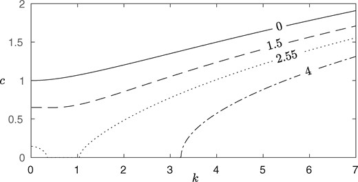
$Dispersion relation (3.12) with parameter values $\mathcal{R}=2$, $\Lambda=3$, $\tau=0.5$. The values of $E_b$ are shown in the figure.$

Fig. 2

Dispersion relation (3.12) with parameter values $R = 2$ ⁠, $Λ = 3$ ⁠, $τ = 0.5$ ⁠. The values of $E_{b}$ are shown in the figure.

Open in new tab Download slide

Below, we consider the general case of dielectric-dielectric, as given by equation (3.12).

4. Weakly nonlinear theory

4.1 Finite long gas layer (shallow–shallow limit)

In this section, the weakly nonlinear theory is investigated under the KdV-scaling for long waves in the case where the upper region is of comparable size to the lower region, that is,

R = O (1)

⁠. The dimensionless variables are defined as follows:

\begin{array}{r} x = l x^{'}, y = h y^{'}, ζ = a ζ^{'}, v = h E_{0} v^{'}, w = h E_{0} w^{'}, \end{array}

(4.1)

\begin{array}{r} t = \frac{l}{\sqrt{g h}} t^{'}, c = \sqrt{g h} c^{'}, ϕ = \frac{g l a}{\sqrt{g h}} ϕ^{'}, \end{array}

(4.2)

where

l

is a typical horizontal lengthscale,

a

is a typical surface amplitude and

\sqrt{g h}

is a typical wave velocity. The dashes are dropped for convenience. We also introduce

\begin{array}{r} α = \frac{a}{h}, β = (\frac{h}{l})^{2}, \end{array}

(4.3)

that are the amplitude and depth parameters respectively. By using the dimensionless variables, the governing equations become

\begin{aligned} β ϕ_{x x} + ϕ_{y y} = 0, & for y < α ζ (x, t), \end{aligned}

(4.4)

\begin{aligned} β v_{x x} + v_{y y} = 0, & for y < α ζ (x, t), \end{aligned}

(4.5)

\begin{aligned} β w_{x x} + w_{y y} = 0, & for y > α ζ (x, t), \end{aligned}

(4.6)

\begin{aligned} ζ_{t} = \frac{1}{β} ϕ_{y} - α ϕ_{x} ζ_{x}, & on y = α ζ (x, t), \end{aligned}

(4.7)

\begin{aligned} ϕ_{y} = 0, & on y = - 1. \end{aligned}

(4.8)

\begin{aligned} w = R, & on y = R, \end{aligned}

(4.9)

\begin{aligned} v = 0 & on y = - 1, \end{aligned}

(4.10)

\begin{aligned} v_{x} + α ζ_{x} v_{y} = w_{x} + α ζ_{x} w_{y} & on y = α ζ (x, t), \end{aligned}

(4.11)

\begin{aligned} v_{y} - α β ζ_{x} v_{x} = Λ (w_{y} - α β ζ_{x} w_{x}) & on y = α ζ (x, t) . \end{aligned}

(4.12)

and

\begin{array}{r} ϕ_{t} + \frac{1}{2} (α ϕ_{x}^{2} + \frac{α}{β} ϕ_{y}^{2}) + ζ - β τ \frac{ζ_{x x}}{(1 + α^{2} β ζ_{x}^{2})^{3 / 2}} + σ_{e} = B, \end{array}

(4.13)

with

\begin{array}{r} σ_{e} = \frac{E_{b} (Λ - 1)}{2 α Λ (1 + α^{2} β ζ_{x}^{2})} (β v_{x}^{2} (Λ + α^{2} β ζ_{x}^{2}) + v_{y}^{2} (α^{2} β Λ ζ_{x}^{2} + 1) + 2 α β (Λ - 1) v_{x} v_{y} ζ_{x}) \end{array}

(4.14)

where

E_{b}

is defined in (3.3). In the KdV-scaling, it is required that

α = β = ϵ

⁠, We expand the functions in powers of

ϵ

by writing

\begin{array}{rcl} ϕ (x, y, t) = ϕ_{0} + ϵ ϕ_{1} + ϵ^{2} ϕ_{2} . . ., \end{array}

(4.15)

\begin{array}{rcl} ζ (x, t) = ζ_{0} + ϵ ζ_{1} + ϵ^{2} ζ_{2} . . ., \end{array}

(4.16)

\begin{array}{rcl} v (x, y, t) = P Λ (y + 1) + ϵ v_{1} + ϵ^{2} v_{2} . . ., \end{array}

(4.17)

\begin{array}{rcl} w (x, y, t) = P (y - R) + R + ϵ w_{1} + ϵ^{2} w_{2} . . ., \end{array}

(4.18)

where the leading order terms in (4.17) and (4.18) are derived in section 3. All the functions are expanded about

y = 0

in the boundary conditions on the surface

y = ϵ ζ

⁠. At order

O (1 / ϵ)

⁠, the Bernoulli constant

B

is found to be

\begin{array}{r} B = - \frac{1}{2} E_{b} P^{2} Λ (1 - Λ) . \end{array}

(4.19)

By solving the Laplace equation (4.5) and (4.6) with (4.9) and (4.10),

v_{1}

and

w_{1}

can be written as

\begin{array}{rcl} v_{1} = (y + 1) A (x, t), \end{array}

(4.20)

\begin{array}{rcl} w_{1} = (y - R) B (x, t) . \end{array}

(4.21)

The

O (ϵ)

balance in the boundary condition (4.12) gives us that

A (x, t) = Λ B (x, t)

⁠. By making use of (4.11) at

O (ϵ)

to solve for

A (x, t)

and collecting the terms of (4.7) and (4.13) at the leading order

O (ϵ^{0})

⁠, the shallow water theory is obtained

\begin{array}{rcl} ζ_{0_{t}} + ϕ_{0_{x x}} = 0, \end{array}

(4.22)

\begin{array}{rcl} c_{0}^{2} ζ_{0_{x}} + ϕ_{0_{x t}} = 0, \end{array}

(4.23)

with

c_{0} = \sqrt{1 - \frac{E_{b} P^{2} (1 - Λ)^{2}}{1 + Λ^{- 1} R}},

(4.24)

which agrees with the long wave speed predicted by the dispersion relation (3.12) in the limit

k \to 0

⁠.

In order to derive the KdV equation, we introduce

X = x - c_{0} t, T = ϵ t .

(4.25)

Then, we are required to simplify the boundary conditions (4.7) and (4.13) at

O (ϵ)

⁠. Solving the Laplace equation (4.4) combined with (4.8) for

ϕ

yields

\begin{array}{rcl} ϕ_{1} = - \frac{(y + 1)^{2}}{2} ϕ_{0_{X X}} + ψ_{1} (X, T), \end{array}

(4.26)

\begin{array}{rcl} ϕ_{2} = \frac{(y + 1)^{4}}{24} ϕ_{0_{X X X X}} - \frac{(y + 1)^{2}}{2} ψ_{1_{X X}}, \end{array}

(4.27)

Similarly, we solve (4.5) and (4.6) with (4.9)–(4.12) for

v

and

w

⁠, and obtain

\begin{array}{rc} v_{2} = Λ (y + 1) V (X, T) - \frac{P (1 - Λ) (y + 1)^{3}}{6 (1 + Λ^{- 1} R)} ζ_{0_{X X}}, \end{array}

(4.28)

\begin{array}{rc} w_{2} = (y - R) W (X, T) - \frac{P (1 - Λ) (y - R)^{3}}{6 (R + Λ)} ζ_{0_{X X}} . \end{array}

(4.29)

By summing the differentiation of (4.13) with respect to

X

and (4.7) multiplied by

c_{0}

and making use of (4.11), (4.12), (4.24),

ψ_{1}

⁠,

ζ_{1}

,

V

and

W

are all eliminated and the electrified Korteweg de-Vries equation is obtained

\begin{array}{r} 2 c_{0} ζ_{0_{T}} + δ ζ_{0_{X X X}} + μ ζ_{0} ζ_{0_{X}} = 0, \end{array}

(4.30)

where

\begin{array}{rcl} δ = \frac{c_{0}^{2}}{3} - τ + \frac{E_{b} P^{2} Λ (1 - Λ)^{2} (R^{3} + Λ)}{3 (R + Λ)^{2}}, \end{array}

(4.31)

\begin{array}{rcl} μ = 3 c_{0}^{2} - \frac{3 E_{b} P^{2} Λ (1 - Λ)^{3}}{(R + Λ)^{2}} . \end{array}

(4.32)

Linearising (4.30) by taking the ansatz (3.8) for $ζ$ ⁠, one recovers a relation between the angular frequency and wavenumber, which, when expanded about $k = 0$ ⁠, agrees with the linear dispersion relation (3.12) up to order $k^{2}$ ⁠. In the absence of the electric field, (4.30) reduces to KdV equation for capillary-gravity waves. In the limit case where $R$ tends to infinity, the $y$ coordinate in the upper layer should be scaled by $l$ rather than $h$ ⁠. Solution (4.21) is invalid since (4.6) becomes a standard Laplace equation for $w$ ⁠. By elementary analysis as shown in (15), the $y$ -derivative of $w_{1}$ is the Hilbert transform of the $x$ -derivative, which finally results in a KdV-Benjamin–Ono equation. The details will be explained in the next subsection.

4.2 Infinitely wide gas layer (shallow-deep limit)

We denote the vertical Cartesian coordinate above the surface

y = ζ (x)

by

Y

⁠. The new scaling is

\begin{array}{r} x = l x^{'}, y = h y^{'}, ζ = a ζ^{'}, v = h E_{0} v^{'}, Y = l Y^{'}, \end{array}

(4.33)

\begin{array}{r} w = l E_{0} w^{'}, t = \frac{l}{\sqrt{g h}} t^{'}, c = \sqrt{g h} c^{'}, ϕ = \frac{g l a}{\sqrt{g h}} ϕ^{'} . \end{array}

(4.34)

The governing equations (4.4), (4.5), (4.7), (4.8) and (4.10) remain unchanged. Equations (4.6), (4.9), (4.11) and (4.12) are respectively updated to

\begin{aligned} w_{x x} + w_{Y Y} = 0, & for Y > α \sqrt{β} ζ (x, t), \end{aligned}

(4.35)

\begin{aligned} w_{Y} \to 1, & as Y \to \infty, \end{aligned}

(4.36)

\begin{aligned} \sqrt{β} v_{x} + α \sqrt{β} ζ_{x} v_{y} = w_{x} + α \sqrt{β} ζ_{x} w_{Y} & on y = α ζ (x, t), \end{aligned}

(4.37)

\begin{aligned} v_{y} - α β ζ_{x} v_{x} = Λ (w_{Y} - α \sqrt{β} ζ_{x} w_{x}) & on y = α ζ (x, t) . \end{aligned}

(4.38)

The fluid part of (4.13) has the same form but the Maxwell stress

σ_{e}

from (4.14) changes to

\begin{array}{r} σ_{e} = \frac{E_{b} (Λ - 1)}{2 α (1 + α^{2} β ζ_{x}^{2})} [w_{x}^{2} (1 + α^{2} β Λ ζ_{x}^{2}) + w_{Y}^{2} (Λ + α^{2} β ζ_{x}^{2}) - 2 α \sqrt{β} (Λ - 1) w_{x} w_{Y} ζ_{x}] . \end{array}

(4.39)

We still have

α = β = ϵ

⁠. The asymptotic expansions for

v

and

w

are given by

\begin{array}{rcl} v = Λ (y + 1) + δ_{1} v_{1} + . . ., \end{array}

(4.40)

\begin{array}{rcl} w = Y + δ_{2} w_{1} + . . . . \end{array}

(4.41)

For the consistency of the boundary conditions (4.37) and (4.38),

δ_{1} = δ_{2} = ϵ^{3 / 2}

is required. Solving the Laplace problem (4.35) and making use of (4.37) and (4.38) yields at

O (ϵ^{3 / 2})

\begin{array}{r} w_{Y} = H [w_{X}] = - (1 - Λ) H [ζ_{0_{X}}], \end{array}

(4.42)

where

H

is the Hilbert transform defined by a Cauchy principal value form as

\begin{array}{r} H [f] (z) = \frac{1}{π} P.V. \int_{- \infty}^{\infty} \frac{f (ξ)}{ξ - z} d ξ . \end{array}

(4.43)

After calculations similar to those in (22), we obtain a KdV-Benjamin–Ono equation

\begin{array}{r} 2 ζ_{0_{T}} + 3 ζ_{0} ζ_{0_{X}} + (\frac{1}{3} - τ) ζ_{0_{X X X}} + {\bar{E}}_{b} Λ (1 - Λ)^{2} H [ζ_{0_{X X}}] = 0, \end{array}

(4.44)

where

{\bar{E}}_{b} = ϵ^{1 / 2} E_{b}

⁠. The linear dispersion relation can be retrieved up to first two orders by expanding (3.13) in a power of

k

⁠. We also note that equation (4.44) agrees with the Boussinesq system derived in (17).

5. Numerical scheme

In this section, we will explain the numerical method used to solve the fully nonlinear system of equations. We will use a boundary integral equation method, following closely the work in (17). The numerical method will be used to study waves of wavelength $λ$ travelling at a constant speed $c$ ⁠. Hence, it is advantageous to take a frame of reference moving with the wave, such that the problem is steady. We parameterise the interface $(X (s), Y (s))$ in $(x, y)$ ⁠, where $s$ is the arclength. We choose the origin such that $x = 0$ is at a point of symmetry of the wave (a crest or a trough), and $y = 0$ is again the mean level of the interface. We choose $s = 0$ at the point $x = 0$ ⁠, and denote the total arclength over a wavelength of the wave as $b$ ⁠.

We wish to reduce the problem to a system of integro-differential equations. The complex velocity

U - i V

is an analytic function of

z = x + i y

⁠, and the no normal flow condition (2.5) on the bottom electrode

y = - 1

states that it is purely real on the real-axis. This allows us to reflect the flow across the boundary using the Schwarz reflection principle. Following (17), we conformally map the flow domain and its reflection in the

z

-plane

{z = x + i y : - λ / 2 < x < λ / 2, - 2 - ζ (x) < y < ζ (x)}

to an annulus

Ω_{1}

in the

t_{1}

-plane, via the function

t_{1} = e^{- k i z} = e^{- k i x} e^{k y},

(5.1)

where

k = 2 π / λ

is the wavenumber. We apply Cauchy’s integral equation to the function

U - i V

⁠, taking the domain to be the annulus

Ω_{1}

in the

t_{1}

-plane. After some algebra, and making use of the assumed symmetry of the wave (⁠

X (s) = - X (s)

⁠,

Y (s) = Y (- s)

etc.), we find that the real part of the equation gives that

\begin{aligned} \frac{π}{k} U (s_{0}) & = \int_{0}^{b / 2} \frac{χ_{1} (U, V) (1 - R_{-} \cos Θ_{-}) + χ_{2} (U, V) R_{-} \sin Θ_{-}}{1 + R_{-}^{2} - 2 R_{-} \cos Θ_{-}} d s \\ + \int_{0}^{b / 2} \frac{χ_{1} (U, V) (1 - R_{-} \cos Θ_{+}) - χ_{2} (U, V) R_{-} \sin Θ_{+}}{1 + R_{-}^{2} - 2 R_{-} \cos Θ_{+}} d s \\ - \int_{0}^{b / 2} \frac{χ_{1} (U, V) (1 - e^{2 k} R_{+} \cos Θ_{-}) - χ_{2} (U, V) R_{+} \sin Θ_{-}}{1 + R_{+}^{2} - 2 R_{+} \cos Θ_{-}} d s \\ - \int_{0}^{b / 2} \frac{χ_{1} (U, V) (1 - R_{+} \cos Θ_{+}) + χ_{2} (U, V) R_{+} \sin Θ_{+}}{1 + R_{+}^{2} - 2 R_{+} \cos Θ_{+}} d s \end{aligned}

(5.2)

where

\begin{array}{r} R_{-} = e^{k (Y (s_{0}) - Y (s))}, R_{+} = e^{2 k + k (Y (s_{0}) + Y (s))} Θ_{\pm} = k (X (s_{0}) \pm X (s)), \end{array}

(5.3)

and

\begin{array}{r} χ_{1} (U, V) = U (s) X_{s} (s) + V (s) Y_{s} (s), χ_{2} (u, v) = U (s) Y_{s} (s) - V (s) X_{s} (s) . \end{array}

(5.4)

This is similar to equation (4.12) seen in (17). The above integral is a Cauchy principal value.

Since

v

and

w

are scalar potentials of irrotational and incompressible vector fields, we can write them as the real parts of complex analytic functions,

F_{1} (z) = v (z) + i ξ (z), F_{2} = w (z) + i ν (z),

(5.5)

where

ξ

and

ν

are the harmonic conjugates of

v

and

w

respectively. The harmonic potentials satisfy the Cauchy Riemann equations, given by

\begin{array}{r} v_{x} = ξ_{y}, v_{y} = - ξ_{x}, w_{x} = ν_{y}, w_{y} = - ν_{x} . \end{array}

(5.6)

The derivatives of $F_{1}$ and $F_{2}$ are analytic, and hence making use of (5.6), we find that $ξ_{x} - i ξ_{y}$ and $ν_{x} - i ν_{y}$ are also analytic functions. Furthermore, the boundary conditions on the electrodes (2.6) and (2.7), combined with (5.6), imply that $ξ_{y} = 0$ and $ν_{y} = 0$ on $y = - 1$ and $y = R$ respectively. Hence, we can apply the Schwarz reflection principle to find the analytic continuation of $ξ_{x} - i ξ_{y}$ across $y = - 1$ and $ν_{x} - i ν_{y}$ across $y = R$ ⁠.

We apply Cauchy’s integral equation to the function

ξ_{x} - i ξ_{y}

⁠, taking domain to be again the annulus

Ω_{1}

in the

t_{1}

-plane. Taking the real parts of this equation, one finds

\begin{aligned} \frac{π}{k} ξ_{x} (s_{0}) & = \int_{0}^{b / 2} \frac{χ_{1} (ξ_{x}, ξ_{y}) (1 - R_{-} \cos Θ_{-}) + χ_{2} (ξ_{x}, ξ_{y}) R_{-} \sin Θ_{-}}{1 + R_{-}^{2} - 2 R_{-} \cos Θ_{-}} d s \\ + \int_{0}^{b / 2} \frac{χ_{1} (ξ_{x}, ξ_{y}) (1 - R_{-} \cos Θ_{+}) - χ_{2} (ξ_{x}, ξ_{y}) R_{-} \sin Θ_{+}}{1 + R_{-}^{2} - 2 R_{-} \cos Θ_{+}} d s \\ - \int_{0}^{b / 2} \frac{χ_{1} (ξ_{x}, ξ_{y}) (1 - e^{2 k} R_{+} \cos Θ_{-}) - χ_{2} (ξ_{x}, ξ_{y}) R_{+} \sin Θ_{-}}{1 + R_{+}^{2} - 2 R_{+} \cos Θ_{-}} d s \\ - \int_{0}^{b / 2} \frac{χ_{1} (ξ_{x}, ξ_{y}) (1 - R_{+} \cos Θ_{+}) + χ_{2} (ξ_{x}, ξ_{y}) R_{+} \sin Θ_{+}}{1 + R_{+}^{2} - 2 R_{+} \cos Θ_{+}} d s, \end{aligned}

(5.7)

To obtain a boundary integral equation relating to the electric potential in the gas region, we conformally map the upper region and its reflection across

y = R

to an annulus

Ω_{2}

in the

t_{2}

-plane via the mapping

t_{2} = e^{k i z} = e^{k i x} e^{- k y} .

(5.8)

We then apply Cauchy’s integral equation to the function

ν_{x} - i ν_{y}

in the annular region of the

t_{2}

-plane. Taking real parts of the integral equation, one finds that

\begin{aligned} \frac{π}{k} ν_{x} (s_{0}) & = \int_{0}^{b / 2} \frac{χ_{1} (ν_{x}, ν_{y}) (1 - {\hat{R}}_{-} \cos {\hat{Θ}}_{-}) - χ_{2} (ν_{x}, ν_{y}) {\hat{R}}_{-} \sin {\hat{Θ}}_{-}}{1 + {\hat{R}}_{-}^{2} - 2 {\hat{R}}_{-} \cos {\hat{Θ}}_{-}} d s \\ + \int_{0}^{b / 2} \frac{χ_{1} (ν_{x}, ν_{y}) (1 - {\hat{R}}_{-} \cos {\hat{Θ}}_{+}) + χ_{2} (ν_{x}, ν_{y}) {\hat{R}}_{-} \sin {\hat{Θ}}_{+}}{1 + {\hat{R}}_{-}^{2} - 2 {\hat{R}}_{-} \cos {\hat{Θ}}_{+}} d s \\ - \int_{0}^{b / 2} \frac{χ_{1} (ν_{x}, ν_{y}) (1 - {\hat{R}}_{+} \cos {\hat{Θ}}_{-}) + χ_{2} (ν_{x}, ν_{y}) {\hat{R}}_{+} \sin {\hat{Θ}}_{-}}{1 + {\hat{R}}_{+}^{2} - 2 {\hat{R}}_{+} \cos {\hat{Θ}}_{-}} d s \\ - \int_{0}^{b / 2} \frac{χ_{1} (ν_{x}, ν_{y}) (1 - {\hat{R}}_{+} \cos {\hat{Θ}}_{+}) - χ_{2} (ν_{x}, ν_{y}) {\hat{R}}_{+} \sin {\hat{Θ}}_{+}}{1 + {\hat{R}}_{+}^{2} - 2 {\hat{R}}_{+} \cos {\hat{Θ}}_{+}} d s, \end{aligned}

(5.9)

where

{\hat{R}}_{-} = e^{- k (Y (s_{0}) - Y (s))}, {\hat{R}}_{+} = e^{2 k R - k (Y (s_{0}) + Y (s))}, {\hat{Θ}}_{\pm} = k (X (s_{0}) \pm X (s)) .

(5.10)

Consider a wave whose interface has a length

b

per wavelength

λ

⁠. We discretise

s

into

N

equally spaced meshpoints

s_{i}

over a half wavelength, given by

s_{i} = \frac{(i - 1) b}{2 N}, i = 1, 2, . . ., N .

(5.11)

Denote the

N - 1

midpoints as

s_{i}^{m}

where

s_{i}^{m} = \frac{s_{i} + s_{i + 1}}{2}, i = 1, 2, . . ., N - 1.

(5.12)

The values of

X_{s}

⁠,

Y_{s}

⁠,

U

⁠,

V

⁠,

ν_{x}

and

ν_{y}

at each meshpoint are unknown. One can express the derivatives of

v

and

w

in terms of

ξ

and

ν

using equations (5.6) One can then find

ξ_{x}

and

ξ_{y}

in terms of

ν_{x}

and

ν_{y}

by rearranging the boundary conditions (2.8) and (2.9), to find that

\begin{aligned} ξ_{x} & = (1 + η_{x}^{2})^{- 1} [ν_{y} η_{x} (Λ - 1) + ν_{x} (η_{x}^{2} + Λ)], \end{aligned}

(5.13)

\begin{aligned} ξ_{y} & = (1 + η_{x}^{2})^{- 1} [ν_{y} (η_{x}^{2} Λ + 1) + ν_{x} η_{x} (Λ - 1)] . \end{aligned}

(5.14)

Since we are seeking periodic solutions, we can express the unknowns in a Fourier series, which we truncate after a finite number of terms as follows

\begin{aligned} X_{s} (s) & = \sum_{n = 0}^{N} a_{n} \cos (\frac{2 π n}{b} s), & Y_{s} (s) & = \sum_{n = 1}^{N - 1} b_{n} \sin (\frac{2 π n}{b} s), \\ U (s) & = \sum_{n = 0}^{N} c_{n} \cos (\frac{2 π n}{b} s), & V (s) & = \sum_{n = 1}^{N - 1} d_{n} \sin (\frac{2 π n}{b} s), \\ ν_{x} (s) & = \sum_{n = 0}^{N} e_{n} \cos (\frac{2 π n}{b} s), & ν_{y} (s) & = \sum_{n = 1}^{N - 1} f_{n} \sin (\frac{2 π n}{b} s) . \end{aligned}

(5.15)

Fixing

λ

⁠,

τ

⁠,

R

⁠,

E_{b}

⁠,

Λ

and the amplitude

A

⁠, we have

6 N + 1

unknowns: the coefficients of the Fourier series

a_{n}, \dots, f_{n}

⁠, the Bernoulli constant

B

⁠, the length of the wave

b

⁠, the value

H = Y (0)

and the wavespeed

c

⁠. We satisfy the boundary integral equations (5.2), (5.7) and (5.9) at the midpoints

s_{i}^{m}

⁠. The integrals are Cauchy-principle value, and are evaluated using the trapezoidal rule. This results in

3 N - 3

discrete equations. By the definition of arclength, we have that

X_{s} (s)^{2} + Y_{s} (s)^{2} = 1.

(5.16)

Furthermore, the boundary condition (2.4) can be written as

U (s) Y_{s} (s) - V (s) X_{s} (s) = 0.

(5.17)

We fix the amplitude by satisfying

A = Y (s_{N}) - Y (s_{1}),

(5.18)

and the mean depth of the interface to

0

by setting

\int_{0}^{b / 2} Y (s) X_{s} (s) d s = 0.

(5.19)

We define the wavespeed

c

as the average horizontal velocity for a constant value of

y = a

⁠,

c = \frac{2}{λ} \int_{0}^{λ / 2} U d x .

(5.20)

Irrotationality of the velocity field implies that the equation (5.20) is independent of the value

a

⁠. One can then show

c = \frac{2}{λ} \int_{0}^{b / 2} U (s) X_{s} (s) + V (s) Y_{s} (s) d s .

(5.21)

We fix the wavelength

λ

via the equation

λ = 2 \int_{0}^{b / 2} X_{s} (s) d s .

(5.22)

We need to fix the potential difference between the two electrodes. In the previous sections, we fixed the potential difference (after non-dimensionalisation) across the electrodes to be

R

⁠. This is an integral condition, which for a fixed

x = a

⁠, is given by

R = \int_{0}^{η (x)} v_{y} d y + \int_{η (x)}^{R} w_{y} d y .

(5.23)

However, this condition is numerically expensive to enforce, since it involves evaluating terms within the fluid and gas domains. It is numerically easier to fix the variation in the complex conjugates of

v

and

w

across a wavelength for a fixed

y

⁠. As with the velocity field, the electric fields are both irrotational and incompressible, and hence this integral is independent on the value of

y

⁠. Hence, we fix a constant

p

⁠, defined as

p = 2 \int_{0}^{b / 2} ν_{x} X_{s} + ν_{y} Y_{s} d x .

(5.24)

We choose

p = - P λ

⁠, where

P

is defined in section 3 of the article. This choice of

p

ensures that, for an undisturbed surface, the potential difference between the two electrodes is exactly equal to

R

⁠, and hence numerical results in the following section agree with the linear theory (for example, the dispersion relation (3.12)) of section 3 for small values of the amplitude. The potential difference of a solution can then be obtained by evaluating the integral on the right-hand side of equation (5.23). Finally, Bernoulli’s equation, written in terms of the unknowns (5.15) and satisfied at

s = s_{i}

⁠, becomes

\frac{1}{2} (U^{2} + V^{2}) + \int_{0}^{s_{i}} Y_{s} (s) d s + τ (X_{s} Y_{s s} - Y_{s} X_{s s}) + σ_{e} = B

(5.25)

As stated before, satisfying the three Cauchy integrals (5.2), (5.7) and (5.9) at the midpoints $s_{i}^{m}$ results in $3 N - 3$ equations. We satisfy equations (5.16) and (5.25) at the meshpoints $s_{i}$ ⁠, and (5.17) at the midpoints $s_{i}^{m}$ ⁠. This results in a further $3 N - 1$ equations. Finally, we satisfy (5.18), (5.19), (5.20), (5.22) and (5.24), resulting in $6 N + 1$ equations for the $6 N + 1$ unknowns. We solve this discrete nonlinear system via Newton’s method, where we terminate the iterative procedure once the $L^{\infty}$ norm of the residuals is $O (10^{- 11})$ ⁠.

As well as periodic waves, we also wish to compute solitary waves. One could rewrite the integrals (5.2), (5.7) and (5.9) by using a different conformal mapping to map the domains onto finite width strips in the

t

-plane. Another commonly used method (for example, see (27)) is to approximate solitary waves as long periodic waves. This is the method we shall adopt in this paper. When computing solitary waves, we replace (5.19) with a flat far-field condition

Y (s_{1}) = 0.

(5.26)

In the following section, we discuss the numerical results of periodic waves, solitary waves and generalised solitary waves.

6. Numerical results

We have tested the numerical method for a variety of parameter values. Most of the results that follow will have the following parameters:

E_{b} = 1.5, Λ = 3, R = 2.

(6.1)

The value of $δ$ and $μ$ from equation (4.31) in this instance is given by $δ = 0.5637 - τ$ and $μ = 1.9632$ ⁠. Hence, the value of $δ$ changes sign according to the value of $τ$ ⁠. Three different regimes are possible depending on the value of $τ$ ⁠,

when $τ < 0.1315$ ⁠, the fluid system is destabilised for some wavenumber.
when $0.1315 < τ < 0.5637$ ⁠, the linear phase speed admits a positive minimum. The associated KdV equation (4.30) admits elevation soliton solutions.
when $τ > 0.5637$ ⁠, the linear phase speed is monotonically increasing. The associated KdV equation (4.30) admits depression soliton solutions.

The minimum of the phase speed equals zero when $τ = 0.1315$ ⁠. When $τ < 0.1315$ ⁠, we find that the flow configuration is unstable (the value of $c^{2}$ in the dispersion relation (3.12) is negative for some values of $k$ ⁠). Meanwhile, for $τ$ being above (below) the critical value $0.5637$ ⁠, $δ$ is negative (positive) and the KdV equation (4.30) admits depression (elevation) soliton solutions. Figure 3 shows the dispersion relation for values of $τ$ in these three regimes. In the critical case $τ = 0.5637$ ⁠, the standard KdV equation is invalid as the dispersive term from (4.30) vanishes. A fifth-order KdV equation can be derived under such circumstance, which is not explored in this work. Varying the values of the parameters shown in equation (6.1) changes the values of $τ$ for which these regime changes occur. In particular, increasing $E_{b}$ increases the value of $τ$ for which there exists unstable modes. This is due to the electric field destabilising the flow, while the surface tension is a stabilising force.

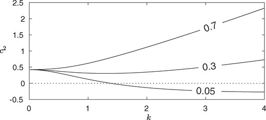
$Dispersion relation (3.12) with the parameter values given by equation (6.1), with varying values of $\tau$ (as shown in the figure). When the curve goes below $c^2=0$ (given by the dotted line), the configuration is linearly unstable.$

Fig. 3

Dispersion relation (3.12) with the parameter values given by equation (6.1), with varying values of $τ$ (as shown in the figure). When the curve goes below $c^{2} = 0$ (given by the dotted line), the configuration is linearly unstable.

Open in new tab Download slide

First, let us explore the regime where the linear phase speed is monotonic. We compare a depression KdV soliton satisfying equation (4.30) with a solution to the full Euler equations with the parameter values given by equation (6.1) and $τ = 1.2$ ⁠. As shown in Fig. 4, the agreement is very satisfactory. Such convincing results ensure that our codes based on the numerical scheme are correctly composed. We also show in the figure a full Euler solution with the same parameter values, except $E_{b} = 0$ ⁠. It can be seen that the solution with the electric field is less steep than the gravity-capillary solitary wave. While there is little difference in the profiles, the effect on the speed of the wave is dramatic. The $E_{b} = 0$ solution has $c = 0.915$ ⁠, while the $E_{b} = 1.5$ solution has $c = 0.5578$ ⁠. Increasing $E_{b}$ further, one finds that the speed of the soliton approaches zero. This is shown in Fig. 5, where we have fixed $A = - 0.2$ and allowed $E_{b}$ to vary. A relationship between $E_{b}$ and $c$ is found. The points $(a)$ and $(b)$ on the figure correspond to the solutions shown in Fig. 4.

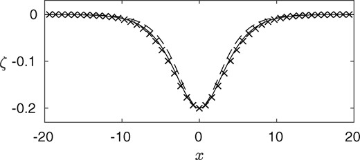
$Comparison of computations for a depression soliton with $A=-0.2$, $\lambda=80$, $E_b=1.5$, $\Lambda=3$, $\mathcal{R}=2$ and $\tau=1.2$ by the full Euler (solid line) and by (4.30) (crosses). The dashed curve is a full Euler solution with $E_b=0$.$

Fig. 4

Comparison of computations for a depression soliton with $A = - 0.2$ ⁠, $λ = 80$ ⁠, $E_{b} = 1.5$ ⁠, $Λ = 3$ ⁠, $R = 2$ and $τ = 1.2$ by the full Euler (solid line) and by (4.30) (crosses). The dashed curve is a full Euler solution with $E_{b} = 0$ ⁠.

Open in new tab Download slide

$A branch of depression solitons with $A=-0.2$, $\Lambda=3$, $\mathcal{R}=2$ and $\tau=1.2$. We see that, as $E_b$ is increased, the speed of the wave decreases, until eventually no depression soliton solutions are found for $E_b>2.39$. The points $(a)$ and $(b)$ correspond to the solid and dashed curve in Fig. 4, respectively.$

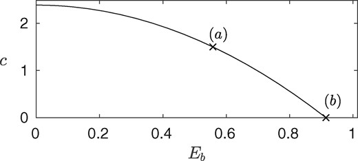
Fig. 5

A branch of depression solitons with $A = - 0.2$ ⁠, $Λ = 3$ ⁠, $R = 2$ and $τ = 1.2$ ⁠. We see that, as $E_{b}$ is increased, the speed of the wave decreases, until eventually no depression soliton solutions are found for $E_{b} > 2.39$ ⁠. The points $(a)$ and $(b)$ correspond to the solid and dashed curve in Fig. 4, respectively.

Open in new tab Download slide

Next, consider the regime, where the dispersion relation experiences a minimum $c = c * > 0$ ⁠. We compute solitary wavepackets in the full Euler regime. By (29), these solutions can be approximated by the associated Nonlinear Schrödinger (NLS) Equation’s solitary wave solution at small amplitude. Both elevation and depression solitary wave packets bifurcate from the minimum of the dispersion relation by (30). Without any knowledge on the NLS, an alternative approach to discover these solitary waves is to apply an artificial Gaussian pressure to the free-surface, and find solutions with $c < c^{*}$ which are perturbations to the uniform stream (characterised by small amplitudes). We then follow the branch of solutions with an artificial pressure to larger amplitudes. Once a suitably large solution is found, one can use this solution as an initial guess for a solitary wave packet with no artificial pressure. This trick has been used in previous literature, for example in (31). Here, we only show the existence of the wavepackets as presented in Fig. 6. The rigorous analysis of these waves requires a future study on the NLS.

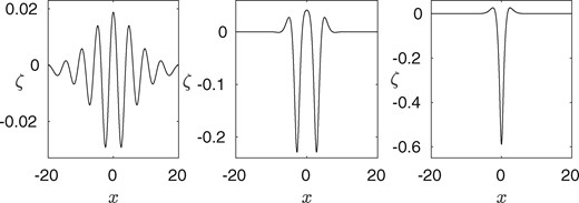
$Solitary wavepacket profiles. All have parameter values given by (6.1), and $\tau=0.3$. The figures on the left and in the centre are elevation solitary waves, while the figure on the right is a depression solitary wave.$

Fig. 6

Solitary wavepacket profiles. All have parameter values given by (6.1), and $τ = 0.3$ ⁠. The figures on the left and in the centre are elevation solitary waves, while the figure on the right is a depression solitary wave.

Open in new tab Download slide

We seek non-resonant periodic waves with $τ = 0.4$ by using a linear solution as the initial guess in Newton’s method. The continuation over the amplitude is shown in the left graph of Fig. 7. The corresponding wave profiles are plotted on the right. Highly nonlinear solution possess a sharp trough and a broad crest. We follow to find resonant periodic waves with the same inverse Bond number and $A = 0.05$ by choosing the value of $λ$ from (3.12) such that the solution experiences second, third, fourth and fifth mode resonance respectively as presented in Fig. 8(a)–(d).

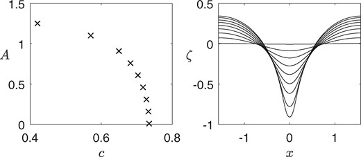
$Computations for periodic waves with $\lambda=\pi$, $E_b=1.5$, $\Lambda=3$, $\mathcal{R}=2$, $\tau=0.4$ and various values of $A$. The figure on the left is the amplitude-speed diagram. The associated wave profiles are shown in the rightmost figure.$

Fig. 7

Computations for periodic waves with $λ = π$ ⁠, $E_{b} = 1.5$ ⁠, $Λ = 3$ ⁠, $R = 2$ ⁠, $τ = 0.4$ and various values of $A$ ⁠. The figure on the left is the amplitude-speed diagram. The associated wave profiles are shown in the rightmost figure.

Open in new tab Download slide

$Typical wave profiles of resonant periodic solutions with $E_b=1.5$, $\Lambda=3$, $\mathcal{R}=2$, $\tau=0.4$ and $A=0.05$. The value of $\lambda$ is chosen such that the solution experiences second, third, fourth and fifth mode resonance respectively for graphs $(a)$–$(d)$.$

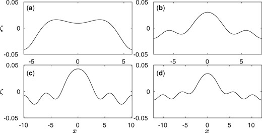
Fig. 8

Typical wave profiles of resonant periodic solutions with $E_{b} = 1.5$ ⁠, $Λ = 3$ ⁠, $R = 2$ ⁠, $τ = 0.4$ and $A = 0.05$ ⁠. The value of $λ$ is chosen such that the solution experiences second, third, fourth and fifth mode resonance respectively for graphs $(a)$ – $(d)$ ⁠.

Open in new tab Download slide

Additionally, due to the presence of a phase speed minimum, resonance of the long wave (elevation soliton as predicted by the associated KdV) with a short wave occurs at zero wavenumber resulting in non-decaying oscillatory ripples in the tail. These solutions are called generalised solitary wave, and they can be found numerically by extending the wavelength of a periodic solution with speed greater than the long wave speed. As one increases the wavelength more ripples appear in the far field. We stop the numerical procedure when there is minimal change in the profile as the wavelength is further increased. Further by a continuation on the branch, a complete diagram is obtained for $τ = 0.4$ as presented in Fig. 9. The wavelength chosen here is $69.83$ ⁠, and the corresponding phase speed from the linear dispersion relation (3.12) is about $0.6501$ ⁠. When the amplitude is close to zero, the branch approaches the predicted phase speed marked by a circle. The associated long wave speed from (4.24) is $0.6512$ marked by a diamond. The difference between the values stems from the fact that we have approximated generalised solitary waves with solutions of finite wavelength. The gap between the circle and the diamond is decreased as the wavelength is increased. In the limit of long wave, these two points collapse. Two typical wave profiles are plotted on the right of the figure. Despite of the almost flat surface in the tail, profile $(a)$ is not an embedded soliton since there are still tiny ripples of size comparable to the numerical error from Newton’s method.

$The figure on the left is an amplitude-speed diagram of the generalised elevation solitary waves with $E_b=1.5$, $\tau=0.4$, $\mathcal{R}=2$, $\Lambda=3$ and $\lambda=69.83$. The phase speed predicted by the dispersion relation is marked a circle on the axis. The long wave speed is marked as a diamond. The corresponding profiles for the waves which are marked by a cross in the left graph are shown in the right three figures.$

Fig. 9

The figure on the left is an amplitude-speed diagram of the generalised elevation solitary waves with $E_{b} = 1.5$ ⁠, $τ = 0.4$ ⁠, $R = 2$ ⁠, $Λ = 3$ and $λ = 69.83$ ⁠. The phase speed predicted by the dispersion relation is marked a circle on the axis. The long wave speed is marked as a diamond. The corresponding profiles for the waves which are marked by a cross in the left graph are shown in the right three figures.

Open in new tab Download slide

7. Conclusion

In conclusion, we have presented linear, weakly nonlinear and fully nonlinear solutions to the generalised problem of interfacial waves between a fluid and gaseous dielectric, in the presence of a vertical electric field. The linear regime under various settings has been illustrated and summarised. Korteweg de-Vries equation has been derived for long waves. A valid numerical scheme of boundary integral equation has been introduced for fully nonlinear computations. Periodic, solitary and generalised solitary waves have been computed. The bifurcation of generalised solitary waves has been discussed in detail.

Acknowledgements

The work was initiated by a MSc dissertation for University College London by J.J.S.K. and achieved during a collaborative research visit of A.D. at University of Bath sponsored by the QJMAM fund for applied mathematics (T.G.). A.D. was also supported under grant EP/M507970/1. J.M.V.D.B. was supported by EPSRC under grant EP/N018559/1.

References

[1]

Taylor

G. I.

,

Disintegration of water droplets in an electric field

,

Proc. R. Soc. A

280

(

1964

)

383

–

397

.

Google Scholar

OpenURL Placeholder Text

WorldCat

[2]

Taylor

G. I.

,

The force exerted by an electric field on a long cylindrical conductor

,

Proc. R. Soc. A

291

(

1965

)

145

–

158

.

Google Scholar

OpenURL Placeholder Text

WorldCat

[3]

Taylor

G. I.

and

Van Dyke

M. D.

,

Electrically driven jets

,

Proc. R. Soc. A

313

(

1969

)

453

–

475

.

Google Scholar

OpenURL Placeholder Text

WorldCat

[4]

Jones

T. B.

,

Electrohydrodynamically enhanced heat transfer in liquids—a review

,

Adv. Heat Transfer

14

(

1979

)

107

–

148

.

Google Scholar

Crossref

WorldCat

[5]

Ghoshal

U.

and

Miner

A. C.

,

Cooling of high power density devices by electrically conducting fluids

.

U.S. Patent

(

2003

)

6,658,861

.

Google Scholar

OpenURL Placeholder Text

WorldCat

[6]

Kistler

S. F.

and

Schweizer

P. M.

,

Liquid Film Coating - Scientific Principles and their Technological Implications

(

Chapman and Hall

,

Springer, New York

1997

).

Google Scholar

Google Preview

OpenURL Placeholder Text

WorldCat

[7]

Griffing

E. M.

,

Bankoff

S. G.

,

Miksis

M. J.

and

Schluter

R. A.

,

Electrohydrodynamics of thin flowing films

,

J. Fluids Eng.

128

(

2006

)

276

–

283

.

Google Scholar

Crossref

WorldCat

[8]

Chen

X.

,

J. Cheng and X. Yin. Advances and applications of electrohydrodynamics

,

Chin. Sci. Bull.

48

(

2003

)

1055

–

1063

.

Google Scholar

Crossref

WorldCat

[9]

Papageorgiou

D. T.

,

Film flows in the presence of electric fields

,

Ann. Rev. Fluid Mech.

51

(

2019

)

155

–

187

.

Google Scholar

Crossref

WorldCat

[10]

Taylor

G.

and

McEwan

A.

,

The stability of a horizontal fluid interface in a vertical electric field

,

J. Fluid Mech.

22

(

1965

)

1

–

15

.

Google Scholar

Crossref

WorldCat

[11]

Melcher

J. R.

and

Schwarz

W. J.

,

Interfacial relaxation overstability in a tangential electric field

,

Phys. Fluids

11

(

1968

)

2604

–

2616

.

Google Scholar

Crossref

WorldCat

[12]

Zubarev

N. M.

and

Kochurin

E.

,

Nonlinear dynamics of the interface between fluids at the suppression of Kelvin-Helmholtz instability by a tangential electric field

,

JETP Lett.

104

(

2016

)

275

–

280

.

Google Scholar

Crossref

WorldCat

[13]

Barannyk

L. L.

,

Papageorgiou

D. T.

and

Petropoulos

P. G.

,

Suppression of Rayleigh-Taylor instability using electric fields

,

Math. Comp. Simul.

82

(

2012

)

1008

–

1016

.

Google Scholar

Crossref

WorldCat

[14]

Cimpeanu

R.

,

Papageorgiou

D. T.

and

Petropoulos

P. G.

,

On the control and suppression of the Rayleigh-Taylor instability using electric fields

,

Phys. Fluids

26

(

2014

)

022105

.

Google Scholar

Crossref

WorldCat

[15]

Papageorgiou

D. T.

,

J.-M. Vanden-Broeck, Large-amplitude capillary waves in electrified fluid sheets

,

J. Fluid Mech.

508

(

2004

)

71

–

88

.

Google Scholar

Crossref

WorldCat

[16]

Papageorgiou

D. T.

,

Petropoulos

P. G.

and

Vanden-Broeck

J.-M.

,

Gravity capillary waves in fluid layers under normal electric fields

,

Phys. Rev. E

72

(

2005

)

051601

.

Google Scholar

Crossref

WorldCat

[17]

Papageorgiou

D. T.

and

Vanden-Broeck

J.-M.

,

Numerical and analytical studies of non-linear gravity–capillary waves in fluid layers under normal electric fields

,

IMA J. Appl. Math.

72

(

2006

)

832

–

853

.

Google Scholar

Crossref

WorldCat

[18]

Easwaran

C.

,

Solitary waves on a conducting fluid layer

,

Phys. Fluids

31

(

1988

)

3442

–

3443

.

Google Scholar

Crossref

WorldCat

[19]

Perelman

T.

,

Fridman

A.

and

Eliashevich

M.

,

Modified Korteweg-de Vries equation in electrohydrodynamics

,

Sov. Phys. JETP

66

(

1974

)

1316

–

1323

.

Google Scholar

OpenURL Placeholder Text

WorldCat

[20]

Hunt

M. J.

and

Vanden-Broeck

J.-M.

,

A study of the effects of electric field on two-dimensional inviscid nonlinear free surface flows generated by moving disturbances

,

J. Eng. Math.

92

(

2015

)

1

–

13

.

Google Scholar

Crossref

WorldCat

[21]

Hammerton

P.

,

Existence of solitary travelling waves in interfacial electrohydrodynamics

,

Wave Motion

50

(

2013

)

676

–

686

.

Google Scholar

Crossref

WorldCat

[22]

Gleeson

H.

,

Hammerton

P.

,

Papageorgiou

D.

and

Vanden-Broeck

J.-M.

,

A new application of the Korteweg-de Vries Benjamin–Ono equation in interfacial electrohydrodynamics

,

Phys. Fluids

19

(

2007

)

031703

.

Google Scholar

Crossref

WorldCat

[23]

Hunt

M.

,

Vanden-Broeck

J.-M.

,

Papageorgiou

D. T.

and

Părău

E.

,

Benjamin–Ono Kadomtsev–Petviashvili’s models in interfacial electro-hydrodynamics

,

Eur. J. Mech.-B/Fluids

65

(

2017

)

459

–

463

.

Google Scholar

Crossref

WorldCat

[24]

Wang

Z.

,

Modelling nonlinear electrohydrodynamic surface waves over three-dimensional conducting fluids

,

Proc. R. Soc.

A 473

(

2017

)

20160817

.

Google Scholar

Crossref

WorldCat

[25]

Gao

T.

,

Milewski

P. A.

,

Papageorgiou

D. T.

and

Vanden-Broeck

J-M.

.

Dynamics of fully nonlinear capillary–gravity solitary waves under normal electric fields

,

J. Eng. Math.

108

(

2018

)

107

–

122

.

[26]

Gao

T.

,

Doak

A.

,

Vanden-Broeck

J.-M.

and

Wang

Z.

,

Capillary-gravity waves on a dielectric fluid of finite depth under normal electric field

,

Eur. J. Mech. B

77

(

2019

)

98

–

107

.

Google Scholar

Crossref

WorldCat

[27]

Dias

F.

,

Capillary–gravity periodic and solitary waves

,

Phys. Fluids

,

6

(

1994

)

2239

–

2241

.

Google Scholar

Crossref

WorldCat

[28]

Wang

Z.

,

Stability and dynamics of two-dimensional fully nonlinear gravity–capillary solitary waves in deep water

,

J. Fluid Mech.

809

,

530

–

552

.

Crossref

WorldCat

[29]

Dias

F.

and

Iooss

G.

,

Capillary-gravity solitary waves with damped oscillations

,

Physica D

65

(

1993

)

399

–

423

.

Google Scholar

Crossref

WorldCat

[30]

Iooss

G.

and

Kirrmann

P.

,

Capillary-gravity waves on the free surface of an inviscid fluid of infinite depth: existence of solitary waves

,

Arch. Rat. Mech. Anal.

(

1996

)

136

,

1

–

19

.

Google Scholar

Crossref

WorldCat

[31]

Vanden-Broeck

J.-M.

and

Dias

F.

,

Gravity-capillary solitary waves in water of infinite depth and related free-surface flows

,

J. Fluid Mech.

240

(

1992

)

549

–

557

.

Google Scholar

Crossref

WorldCat

This article is published and distributed under the terms of the Oxford University Press, Standard Journals Publication Model (https://dbpia.nl.go.kr/journals/pages/open_access/funder_policies/chorus/standard_publication_model)

Download all slides

Month:	Total Views:
June 2020	7
July 2020	8
August 2020	36
September 2020	3
October 2020	6
November 2020	4
December 2020	15
January 2021	11
February 2021	4
March 2021	9
April 2021	1
May 2021	2
July 2021	7
August 2021	4
September 2021	3
October 2021	2
November 2021	1
December 2021	3
February 2022	3
March 2022	8
April 2022	12
May 2022	4
June 2022	19
July 2022	12
August 2022	15
September 2022	15
October 2022	8
November 2022	4
December 2022	16
January 2023	20
February 2023	9
April 2023	4
May 2023	1
June 2023	1
July 2023	5
August 2023	4
October 2023	1
November 2023	2
December 2023	2
February 2024	4
March 2024	3
April 2024	7
December 2024	2
January 2025	3
February 2025	5
March 2025	24
April 2025	8
May 2025	1

Article Contents

Capillary-gravity waves on the interface of two dielectric fluid layers under normal electric fields

Summary

1. Introduction

2. Formulation

3. Linear theory

4. Weakly nonlinear theory

4.1 Finite long gas layer (shallow–shallow limit)

4.2 Infinitely wide gas layer (shallow-deep limit)

5. Numerical scheme

6. Numerical results

7. Conclusion

Acknowledgements

References

Citations

Views

Altmetric

Email alerts

Citing articles via

Latest

Most Read

Most Cited

Article Contents

Capillary-gravity waves on the interface of two dielectric fluid layers under normal electric fields Free

Summary

1. Introduction

2. Formulation

3. Linear theory

4. Weakly nonlinear theory

4.1 Finite long gas layer (shallow–shallow limit)

4.2 Infinitely wide gas layer (shallow-deep limit)

5. Numerical scheme

6. Numerical results

7. Conclusion

Acknowledgements

References

Citations

Views

Altmetric

Email alerts

Citing articles via

Latest

Most Read

Most Cited

This Feature Is Available To Subscribers Only

Capillary-gravity waves on the interface of two dielectric fluid layers under normal electric fields