


Abstract
Accurate calculation of the space charge force inside charged particle beams is of practical concern for a deep understanding of the dynamical evolution of beams propagating in accelerators, especially for high-intensity machines. Many computational schemes have been well developed for space charge calculation. Conventional matrix-based methods are primarily suited for the 2D space charge calculation. However, one major limitation of such methods is that for the 3D case, the matrix representation becomes much more complicated. In this paper, we propose a new method via tensor representation on a discretized 3D map for space charge calculation. With the utilization of the |$n$|-mode product of tensors (orthogonal basis), the 3D Poisson equation can be solved in a concise manner for not only the rectangular domain, but also the nonrectangular case. It is shown that the numerical results of the new method are in good agreement with both the analytical solution of a 3D Gaussian distribution, and the numerical solution of a 2D arbitrary distribution. The paper details the mathematical derivation concerning the tensor-represented Poisson equation, the diagonalization of the Laplacian operator, and the specification of boundary conditions. The proposed method can be applied for solving 3D space charge calculations with sufficient accuracy and efficiency for large-scale 3D simulation of high-intensity beams.
1. Introduction
As one of the most fundamental collective phenomena in particle accelerators, space charge effects refer to the electromagnetic interaction among charged particles in the beams. This interaction manifests itself in a myriad of ways as a defocusing effect, including the formation of halo particles and consequently the growth of beam emittance, beam quality degradation, and, at times, beam collective instability or even beam loss.
In recent years, with increased demand of high-intensity beams for a variety of scientific and industrial applications [1–5], a deep understanding of space-charge-dominated beam dynamics now plays a pivotal role in the design, operation, and optimization of such high-intensity accelerators. In this context, methods for space charge calculation with high efficiency and precision are of practical concern and increasingly sought after in such areas, since these methods can provide detailed information on the dynamical behavior of high-intensity beams.
The essential core for the space charge calculation is the resolution of the Poisson equation. For the most ideal scenarios of a few special particle distributions, such as the uniform (KV) distribution or the Gaussian distribution, the Poisson equation can be solved analytically. These scenarios form the analytical basis for the well-known KV envelope model and the particle-core method (PCM). However, for most realistic beams, solving the Poisson equation analytically becomes a formidable task, since the charged particle distribution is complex and boundary-dependent.
To address this issue, several numerical algorithms have been developed, which usually consist of a particle pusher, a source depositor, and a field solver. The particle pusher and the source depositor can be achieved via the conventional particle-in-cell (PIC) method [6–8]. In this method, the distribution of numerous charged particles in a beam is represented by an ensemble of “macro particles.” These macro particles are interpolated onto a grid (particle pusher), and each grid node is assigned a specific amount of charge (source depositor).
One of the most conventional field solvers is based on the finite difference (FD) method [9–11]. In this method, the Poisson equation is formulated as a differential form. Specifically, with the Laplacian operator discretized as a matrix form, the Poisson equation becomes a set of algebraic equations, and specific boundary conditions can be naturally satisfied. Besides, Green’s function based on the Fast Fourier Transform (FFT) provides us another powerful tool for solving the Poisson equation [12]. In this scheme, the solution is obtained by the integration of Green’s function and the source field. The efficiency of the calculation can be much improved via using the FFT method to treat the integration in the frequency domain. Another field solver to deal with the Poisson equation is the spectral method [13–16]. The idea is to express the solution of the differential equation as the summation of a series of “basis functions” (e.g. a Fourier series with sinusoid functions). The coefficients of the basis functions can be then determined by satisfying the given differential equations.
The most well-adopted spectral scheme is Galerkin’s method developed by Galerkin in 1915, which transforms the continuous equations into discrete forms (e.g. the Sylvester matrix equations) by imposing linear constraints based on the finite sets of basis functions. In the classic literature Ref. [17], Haidvogel and Zang solved the 2D Poisson equation with the Chebyshev polynomials via the Alternating Direction Implicit (ADI) iteration [18] and the matrix diagonalization technique. Recently, Fortunato and Townsend made an extension from the FD discretization to the spectral methods by using the ADI iteration for solving the 2D and 3D Poisson equations [19]. However, for dealing with the 3D case, large matrices are required for implementation of the Kronecker product, which usually causes numerous unnecessary zero elements in the matrices and thus costs much extra computation time. The widely employed matrix representation faces a challenge when extending to the 3D case [20,21].
In this paper we propose a new scheme for 3D space charge calculation based on tensor decomposition and the |$n$|-mode product. By utilizing the technique of tensor decomposition, the discretization issues of 3D and higher Poisson equations can be conveniently represented by higher-order tensors (more details can be found in Appendix A). Originally proposed by Hitchcock in 1927, tensor decomposition is an effective method for tensor analysis [22,23]. In the last ten years, interest in tensor decomposition has fast expanded to many other fields [23,24]. In the proposed scheme, the distribution of charge density and potential are discretized to third-order tensors. The Laplacian operator is represented by the |$n$|-mode product. Various boundary conditions are specified on the surface of the third-order tensors. Furthermore, the computation speed can be largely increased by avoiding the matrix representation.
This article is structured as follows: After the introduction in Section 1, the mathematical derivation of the tensor-decomposition method (TDM) is presented in Section 2. Section 3 discusses the diagonalization of the Laplacian operator and specification of the Poisson equation with several typical boundary conditions. The algorithm flow of 3D space charge calculation is detailed and demonstrated in Section 4, with concrete examples for benchmarking shown in Section 5. A summary is given in Section 6.
2. Discrete axis and maps, the discretized Poisson problem
The Poisson equation in the beam’s rest frame reads
where |$x$| and |$y$| denote the coordinate of the horizontal and vertical direction, respectively, on the transverse plane. |$z$| is the longitudinal direction. |$\nabla ^2$| is the Laplacian operator. |$\varphi (x,y,z)$| is the potential function, |$\rho (x,y,z)$| denotes the charge density, and |$\epsilon _0$| is the vacuum permittivity.
For numerical calculations, the continuous charge distributions are typically discretized to particle lists, and then attributed to discretized grids. For instance, in the PIC method there exist several useful algorithms to obtain the charge on the 3D grid from a distribution of macro particles, such as the Nearest Grid Point (NGP, zero-order interpolation), the Cloud In Cell (CIC, first-order interpolation), and the Triangular Shaped Cloud (TSC, second-order interpolation) [12,25]. In the following, the 3D grid is used for the third-order tensor-generalized calculation.
Firstly, we discretize the Poisson equation on the cube by using the FD method in each one-dimension, given by
in which |$h_{x,y,z}$| denotes the step width in |$x$|, |$y$|, and |$z$|, respectively. The indices |$i,j,k$| are the indices of the grid, with |$1 < i,j,k < N_{x,y,z}$|. Accordingly, the density |$\rho$| should be also discretized with the step width |$h_{x,y,z}$|.
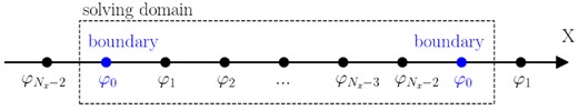
In order to conduct the FD method described in Eq. (2), one can place data points at the grid boundaries, which makes the calculation of derivatives easier. However, we here use a strategy whereby all sampling positions are assumed to be located at the center of each mesh grid, as schematically shown in Fig. 1. The charge of a particle contributes to the density of the two nearest adjacent grids. More specifically, for the particle located at the position |$X_n$| in Fig. 1, the charge is distributed to the mesh nodes |$X_i$| and |$X_{i+1}$| by the CIC (first-order interpolation) method. The advantage of such a discretization manner is that the numerical integration domain remains within the range of 0 to |$L$|, where |$L$| is the maximum length of the integration domain. Consequently, the orthogonality of the discretized basis functions is preserved (further details can be found in Appendix B).
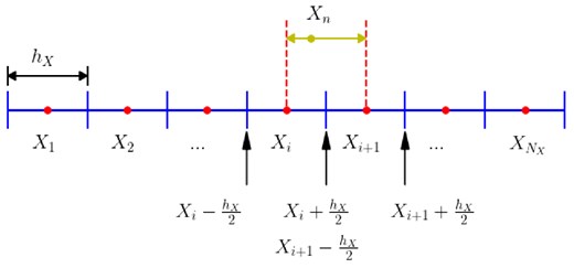
Schematic drawing of particles distributed in the 1D discretized space, in the range of |$0 < X < L_X$|. The first discretized point (|$X_1$|) is at |$h_X/2$| and the last discretized point (|$X_{N_X}$|) is set at |$L_X - h_X/2$|. |$X_n$| denotes the particle in the range of |$X_i < X_n < X_{i+1}$|.
One can see from Eq. (2) that for the 1D Laplacian operator, it can be represented by a convolution kernel |$[1, -2, 1]$|, which is an approximation of the second derivative. For a given vector |$\mathbf {u} = [u_1, u_2, \ldots , u_n]^{\rm T}$|, the convolution at the |$i^{\mathrm{th}}$| point is given by
where |$u_{i-1}$| and |$u_{i+1}$| are the neighboring values of |$u_i$| and |$X$| represents |$x,y,z$|. In terms of the matrix multiplication, in the absence of boundary conditions, such an operation can be written as |$D_X \mathbf {u}$|, with
The matrix representation of the Laplacian in Eq. (3) is widely used in numerical analysis and scientific computing, particularly in solving partial differential equations via FD methods [9]. The explicit expression of |$D_X$| for three typical boundary conditions will be presented in Section 3.
Next, we diagonalize the Laplacian operator |$D_X$| via eigenvalue decomposition, given by
where |$\Lambda _X$| is the diagnosed eigenvalues with |$\Lambda _X \equiv \mathrm{diag}(\lambda _X)$|, and |$U^{(X)}$| the corresponding eigenvectors. With the discretized charge density |$\hat{\rho }$| shown in Fig. 1 and the Laplace operator |$D_X$|, the Poisson equation in Eq. (1) can be converted to the discretized form
The symbol “|$\times _n$|” denotes the |$n$|-mode product (more details can be found in Appendix A). |$\hat{\varphi } \in \mathbf {R}^{N_x \times N_y \times N_z}$| is the discretized potential map to be solved, and |$\hat{\rho } \in \mathbf {R}^{N_x \times N_y \times N_z}$| is the discretized density map that is known to us.
Now we are ready to carry out the higher-order decomposition on both sides of Eq. (5). The decomposed form for |$\hat{\varphi }$| and |$\hat{\rho }$| can be written as, respectively,
Here, |$U^{(X)} \in \mathbf {R}^{N_X \times N_X}$| is a set of discrete basis on which the tensor |$\hat{\varphi }$| is projected with the |$n$|-mode product. |$S \in \mathbf {R}^{N_x \times N_y \times N_z}$| is the coefficient tensor of the discretized potential function to be solved. |$K \in \mathbf {R}^{N_x \times N_y \times N_z}$| is the coefficient tensor of the discretized charge density that can be obtained from a given |$\hat{\rho }$|. |$A$| is the “right-hand-side tensor,” which will be discussed later. Note that the expression in Eq. (7) is for the cases of an ideal metal boundary condition. For other cases, the tensor |$A$| depends on the specified boundary condition, which is detailed and analyzed in Section 3.
With the discretized Poisson equation in Eqs. (5–7), our task is to solve the coefficient tensor |$S$|. We specify the basis |$U^{(1)}$|, |$U^{(2)}$|, and |$U^{(3)}$| to be the eigenvectors |$U^{(x)}$|, |$U^{(y)}$|, and |$U^{(z)}$|, respectively, in Eq. (4) without loss of generality. Combining Eqs. (5–7), we find
Substituting Eq. (4) into Eq. (8), we have
And, performing the |$n$|-mode product operation |$\times _1 U^{(1)-1} \times _2 U^{(2)-1} \times _3 U^{(3)-1}$| on both sides of Eq. (9), we obtain
With the diagonal eigenvalue matrix |$\Lambda _X$|, |$S$| is linearly dependent on |$K$|, and thus Eq. (10) can be written as
where |$i,j,k$| are the indices (|$0< i,j,k < N_X$|), and the eigenvalue |$\lambda _X[i] \equiv \Lambda _X[i,i]$|. Here and in the following text, we use square brackets “[...]” to represent the tensor elements. The tensor |$S$| can be computed via
Finally, the discrete potential function |$\hat{\varphi }$| can be obtained by substituting Eq. (12) into Eq. (6).
3. Diagonalization of Laplace operator and specification of boundary condition
The expressions of |$D_X$| in Eq. (3) with different boundary conditions can be specified as follows (see, e.g. Ref. [26]).
- For the Dirichlet boundary condition with |$u(-h_X) = a$| and |$u(L_X+h_X) = b$|,(13)$$\begin{eqnarray} D_X = \frac{1}{(h_X) ^2} {\begin{pmatrix} -2 &\quad 1 &\quad &\quad &\quad \\ 1 &\quad -2 &\quad 1 &\quad &\quad \\ &\quad \ldots &\quad \ldots &\quad &\quad \\ &\quad &\quad\ldots &\quad \ldots &\quad \\ &\quad 1 &\quad -2 &\quad 1 \\ &\quad &\quad 1 &\quad -2 \\ \end{pmatrix}}. \end{eqnarray}$$
- For the periodic boundary condition with |$u(-h_X) = u(L_X+h_X)$|,(14)$$\begin{eqnarray} D_X = \frac{1}{(h_X) ^2} {\begin{pmatrix}-2 &\quad 1 &\quad &\quad 1\\ 1 &\quad -2 &\quad 1 &\quad &\quad \\ &\quad \ldots &\quad \ldots &\quad &\quad \\ &\quad &\quad\ldots &\quad \ldots &\quad \\ &\quad 1 &\quad -2 &\quad 1 \\ 1 &\quad &\quad 1 &\quad -2 \\ \end{pmatrix}}. \end{eqnarray}$$
- For the Neumann boundary condition with |$\frac{\partial u}{\partial X}(-h_X) = a$| and |$\frac{\partial u}{\partial X}(L_X + h_X) = b$|,(15)$$\begin{eqnarray} D_X = \frac{1}{(h_X) ^2} {\begin{pmatrix}-2 &\quad 2 &\quad &\quad &\quad \\ 1 &\quad -2 &\quad 1 &\quad &\quad \\ &\quad \ldots &\quad \ldots &\quad &\quad \\ &\quad &\quad\ldots &\quad \ldots &\quad \\ &\quad 1 &\quad -2 &\quad 1 \\ &\quad &\quad 2 &\quad -2 \\ \end{pmatrix}}. \end{eqnarray}$$
In order to obtain the orthogonal basis |$U^{(X)}$| in Eq. (4), the Laplace operator by matrix representation |$D_X$| needs to be decomposed either analytically or numerically. For example, the Python module numpy.linalg.svd() [27] can be used to perform the numerical calculation of the eigenvalues |$\Lambda _X$| and eigenvectors |$U^{(X)}$| with three typical boundary conditions.
It should be emphasized that the boundary conditions can be different in the three spatial directions |$x$|, |$y$|, and |$z$|. In practice, the boundary conditions can be flexibly specified. For the simulation of particle beams in accelerators, the periodic condition is usually chosen for the longitudinal direction |$z$|, and the Dirichlet boundary condition is set for the transverse plane |$x$| or |$y$|.
3.1. Dirichlet boundary condition
We first specify the Laplacian operator with the Dirichlet condition, since it is the most common application for beams travelling in accelerators. Figure 2 shows an example of eigenvalues and eigenvectors of the |$D_X$| defined by Eq. (13). One can see the curves of the eigenvalues are cosine-like, while the curves of the eigenvectors are sine-like [28].
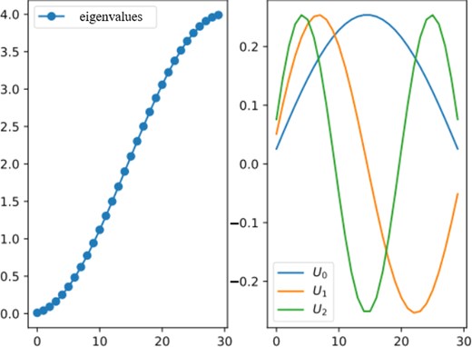
A demonstration of the eigenvalues |$\Lambda _X$| (left) and the first three eigenvectors |$U^{(X)}$| (right) of |$D_X$| with |$N_X=30$|, |$h_X=1$|.
In general, the |$i$|th eigenvalue |$\lambda _X[i]$| can be expressed from Eq. (13) as
and the corresponding |$j$|th component of the |$i$|th eigenvector takes the form
Equation (17) provides a set of sinusoidal function expansions based on the Discrete Sine Transform (DST) [28], which indicates |$U_X$| is an odd function around |$j=-1$| and |$j=N_X$|.
The mesh grid should be defined in such a way that the extrapolated points |$n = -1$| and |$n = N_X$| are located on the metal boundaries. Consequently, the potential on the boundaries is zero.
As mentioned above, the right-side tensor |$A$| defined in Eq. (7) is not simply |$-\hat{\rho }/\epsilon _0$|. In fact, the boundary condition |$\varphi (0)=a, \varphi (L_X)=b$| should be taken into account.
The data volumes of the right-side tensor A are schematically shown in Fig. 3. The green and yellow volumes together represent the data volumes of charge density |$\hat{\rho }$|, with the yellow volume signifying the boundary data that will be replaced by Dirichlet boundary conditions. The blue volume indicates the extrapolated region that will be used to calculate the Dirichlet boundary condition. The implementation of the Dirichlet boundary condition on the yellow volume will be explained in detail below.
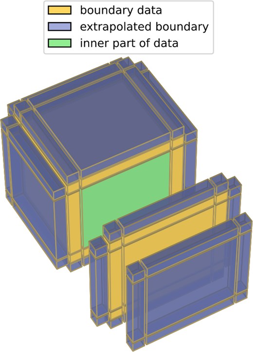
Schematic drawing of the right-side tensor A.
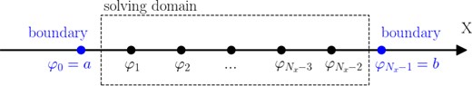
Schematic drawing of 1D Dirichlet boundary condition.
The right-side tensor |$A$| should be treated such that the “shell” (shown as the yellow volume in Fig. 3) of the tensor |$A$| satisfies the Dirichlet boundary condition. For example, in the |$x$|-direction, as schematically shown in Fig. 4, the right-side tensor |$A$| is modified with Eq. (18) and Eq. (19), and becomes |$\tilde{A}$|. Since the boundary condition is independent of the three directions (|$x, y, z$|), for the |$y$|- or |$z$|-direction, the right-side tensor |$A$| has similar modifications.
It is worth pointing out that the values of the elements at the junctions of the volume (|$x=0$|, |$y = 0$|, and |$z = 0$| of the tensor |$A$|) take the form
3.2. Periodic boundary condition
The periodic boundary condition is particularly useful in the scenario when the physical domain is thought to extend infinitely in some directions and can be represented by a finite, repeating unit in a computational model. To avoid the complicated calculation of the complex number, in the following we use a set of bases that contains both of the sine and cosine functions.
The discretized Laplacian operator with the periodic boundary condition can be described by Eq. (14) with its eigenvectors
with the eigenvalue |$\lambda _X$|:
Clearly, with a given periodic boundary condition and an assumed periodic |$\rho$|, the potential |$\phi$| to be solved is also periodic.
As shown in Fig. 5, we can calculate the tensor |$A$| via
Schematic drawing of 1D periodic boundary condition.
Since the periodic boundary condition is explicitly included in the |$D_X$| [see Eq. (14)], it is not necessary to modify the right-hand tensor |$A$| with the periodic boundary condition.
3.3. Neumann boundary condition
The Neumann condition is employed with a given constant electric field at a surface. In this case, the discretized Laplacian operator with the Neumann boundary condition is described by Eq. (15), and its eigenvectors are
with the corresponding |$i$|-th eigenvalue
As shown in Fig. 6, the right-hand tensor |$A$| with the Neumann boundary condition is
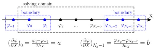
Schematic drawing of 1D Neumann boundary condition.
The values of the elements at the junctions of the volume (|$x=0$|, |$y = 0$|, and |$z = 0$| of the tensor |$A$|) take the form
3.4. Open boundary condition
The open boundary condition is adopted for the case when the domain is not completely enclosed, but extends to infinity in at least one direction. For instance, if the separation between two bunches is sufficiently large, each bunch can be treated as an isolated bunch, and the 1D open boundary conditions can be used to solve Poisson’s equation. In this case, the open boundary condition can be approximated to a closed Dirichlet boundary condition with |$\varphi =0$|, in a sufficiently large computational domain.
However, the large computational domains result in a large cost of computational resources, and such approximations always reduce the accuracy of the numerical results. To address this issue, we propose to utilize a smaller boundary domain that is close to the bunch edge. The value of |$\varphi$| in the boundary domain can be formally obtained from a 3D integral,
where |${\bf r}$| is the spatial coordinate of a mesh point that is outside and near the boundary 0 and |$N_X$|. If the metal boundary is involved, the mirror charge distributed outside of the domain also should be taken into account in |$\rho$|. As shown in Fig. 3, the potential value on any mesh nodes that satisfy one of the following conditions should be given:
Indeed, setting a Dirichlet boundary in this way requires a lot of computation. Fortunately, only the surface nodes of a 3D volume need to be calculated, which can largely reduce the computation cost. In practice, for the simulation of particles propagating in ideal metal beam pipes, the charge density on the metal boundary can be set to zero to simplify the computation.
3.5. Noncube boundary shapes
Equations (13–15) represent the 1D discretized Laplace operators with three typical boundary conditions. This is applicable for cases with a rectangular domain, for which boundary conditions can be implemented to different 1D operators. For instance, with a transverse open boundary and longitudinal period boundary [i.e. the expressions of |$D_z$| take the form in Eq. (14), while |$D_x$| and |$D_y$| are in the form in Eq. (13)], the discretized potential |$\hat{\varphi }$| and discretized charge distribution |$\hat{\rho }$| take the 3D tensor form, and the discretized formula in Eq. (5) is still valid for solving the Poisson equation.
In practice, however, the cross section profile of the beam pipe is usually round, elliptical, or other special shapes (such as racetrack). In those cases, Eq. (5) is inapplicable since the boundary conditions cannot be implemented via simply specifying the form of |$D_x$| and |$D_y$|. As an example, the profile of a nonrectangular beam pipe is shown in Fig. 7. The blue curve represents the profile of a nonrectangular beam pipe. In our method, the potential values |$\varphi _0$| at the nonrectangular boundaries are well approximately represented by the nearest mesh grids. By setting such a boundary condition, the discretized Poisson equation takes the form
Here, the superscript symbol “|$*$|” denotes the map discretized in a 2D tensor, i.e. |$\hat{\varphi }^{*}, \hat{\rho }^{*} \in \mathbf {R}^{N_xN_y \times N_z}$|. The symbol “|$\otimes$|” denotes the Kronecker product (here, |$I_y \otimes D_x + D_y \otimes I_x$| is the operator of the five-point method in the FD method). |$I_{x,y} \in \mathbf {R}^{N_{x,y} \times N_{x,y}}$| are the identity matrices. The expression for |$D_x$|, |$D_y$|, and |$D_z$| in Eq. (13), Eq. (14), or Eq. (15) depends on the specified boundary conditions. The steps for solving Eq. (30) are identical to those for Eq. (5) in Section 2.
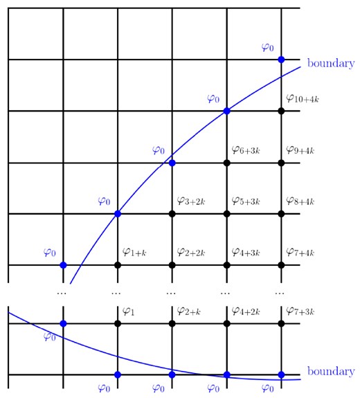
Schematic drawing of 2D nonrectangular boundary condition.
4. Algorithm flow
In the practical application of solving the Poisson equation based on the tensor-generalized spectral method described above, a major error source is the choice of the boundary conditions. In accelerators, a train of charged particle bunches are produced, accelerated, and transported in an ideal metal. The image charge of a beam affects the motion of the beam. As a result, the Dirichlet boundary condition is usually chosen for solving the Poisson equation in the transverse plane. In some accelerators such as Radio-Frequency Quadruples (RFQ), where the bunches are separated by a short distance, one needs to use the longitudinal periodic boundary condition to model a single bunch.
For a specified discrete charge density map |$\hat{\rho }$| with given boundary conditions, the discrete Poisson equation in the beam’s rest frame can be solved via the following steps:
Obtain the basis |$U^{(1)}$|, |$U^{(2)}$|, and |$U^{(3)}$| with eigendecomposition based on Eq. (4), and store them as a constant;
Define the right-side tensor |$A=-\hat{\rho }/\epsilon _0$| with the given boundary condition;
Calculate the coefficient tensor |$K$| by |$K=A\times _1 U^{(1)-1}\times _2 U^{(2)-1}\times _3 U^{(3)-1};$|
Multiply |$K[i,j,k]$| with |$1/(\lambda _x[i]+\lambda _y[j]+\lambda _z[k])$| to obtain |$S$| based on Eq. (12);
Obtain the potential map |$\hat{\varphi }$| via projecting |$S$| to |$U^{(1)}$|, |$U^{(2)}$|, and |$U^{(3)}$| with Eq. (6).
The TDM outlined in the above five steps has a computational complexity of |$O (N_x N_y N_z (N_x + N_y + N_z))$|. In practice, the TDM can be adopted to solve the 3D Poisson equation in a 3D tensor product domain that has identical Dirichlet boundary conditions in two directions (transverse) and periodicity in the other one direction (longitudinal). The algorithm of the TDM is summarized as follows:
Store the charge density map as a tensor |$\rho$|;
Choose the Laplacian operator |$D_X$| based on the specified boundary conditions;
Specify |$\rho$| with a chosen boundary condition;
Obtain the basis |$U^{(X)}$| according to the |$D_X$|;
Solve the coefficient tensor |$K$| with Eq. (11);
Obtain the coefficient tensor |$S$| with Eq. (12);
Solve the potential |$\varphi$| with Eq. (6).
The computational complexity (the definition of computational complexity can be found in Ref. [12]) of several useful algorithms for solving the 3D Poisson equation is summarized in Table 1 and Fig. 8. It can be seen that the computational complexity of the proposed TDM is less than those of the FD and ADI. Note that the FD algorithm we compared here is based on a second-order difference scheme without any optimization techniques for matrix computations.
![The computational complexity of the FD method (in yellow), Green’s function based on FFT (FFT; red), fast Poisson solver by ADI [black, where $\epsilon = 10^{-13}$ (solid) or $10^{-1}$ (dashed)], and TDM (blue).](https://oup.silverchair-cdn.com/oup/backfile/Content_public/Journal/ptep/2025/4/10.1093_ptep_ptaf047/1/m_ptaf047fig8.jpeg?Expires=1750225497&Signature=d3Qg42X2r0F8K66Nzhw6rlCFjnxIUsJdQegrRAR4j~DgrvwHtB1riwWyvVRPYzrSxR8GiMvfBTlE554c532i6Vd8p8L00cYhMYswi27QVOEz6OE6i4-QWvSHM9yisNUS97GjIXLC9VGkH5tshRoqdIHHiHqLo~pJu2bDODxjTetn0GnEkY4NpzNmjRPcHi-CUdWbSM93D2vNF3uEJLupHAY1xAuPN-JNk3aYDI5GvjDpeXNaF6mAJJaIrVgJhqLIs9myFOn5pmpbwhgFRejtKstKR6wHpOHYtCBCJags2n9ZTLRpUsnDKzH0lOg374MNwVYddB2X5xggawzSdvhhIw__&Key-Pair-Id=APKAIE5G5CRDK6RD3PGA)
The computational complexity of the FD method (in yellow), Green’s function based on FFT (FFT; red), fast Poisson solver by ADI [black, where |$\epsilon = 10^{-13}$| (solid) or |$10^{-1}$| (dashed)], and TDM (blue).
Comparison of the computational complexity of several typical algorithms.
| Algorithm | Complexity |
|---|---|
| FD | |$O (N^6)$| |
| Green & FFT | |$O(40N^3 {\rm log}_2N)$| |
| ADI | |$O(N^3 ({\rm log}_2N)^3 {\rm log}_2(1/ \epsilon ))$| |
| TDM | |$O (3N^4)$| |
| Algorithm | Complexity |
|---|---|
| FD | |$O (N^6)$| |
| Green & FFT | |$O(40N^3 {\rm log}_2N)$| |
| ADI | |$O(N^3 ({\rm log}_2N)^3 {\rm log}_2(1/ \epsilon ))$| |
| TDM | |$O (3N^4)$| |
5. Benchmarking
In this section, we carry out benchmarking to check the accuracy of the TDM algorithm. Firstly, we create a 3D spherically symmetric Gaussian particle distribution, in which the numerical solution of the potential can be compared with the analytical results. Secondly, a more realistic example of a 2D particle distribution, generated by a transverse multiturn painting injection procedure, is employed for comparison. Finally, a 3D cylinder beam with a transverse round boundary and longitudinal open boundary is discussed and compared with the 2D coasting beam.
5.1. 3D Gaussian distribution with open boundary
The formula for the charge density of a spherically symmetric Gaussian particle distribution |$\rho (r)$| is
in which |$r= \sqrt{x^2+y^2+z^2}$| is the distance to the origin of the Cartesian coordinate system. |$Q$| is the total charge. |$\sigma$| is the root mean square (rms) size for all three dimensions. The solution |$\varphi (r)$| of the Poisson equation for |$\rho (r)$| can be analytically written as
where erf() is the error function.
We create a third-order tensor to store the discretized density |$\hat{\rho }$| in Eq. (5). The parameters of the 3D grid for the tensor are summarized in Table 2, where |$N_X$| is set to provide an adequate numerical resolution for the charge densities and the resulting electric fields. Note that the grid can be set to be arbitrarily asymmetrical for the calculation of the symmetrical distribution. The corresponding analytical solution is stored in another third-order tensor for comparison with the numerical solution.
Example settings of the 3D grid for the tensor.
| coordinate | range [m] | |$N_X$| | |$X_0$| | |$h_X$| [m] | |$\sigma$| [m] |
|---|---|---|---|---|---|
| |$x$| | −1.2 to 1.2 | 125 | 0.0 | 0.019 | 0.11 |
| |$y$| | −1.05 to 1.05 | 125 | 0.0 | 0.019 | 0.11 |
| |$z$| | −0.8 to 0.8 | 160 | 0.0 | 0.01 | 0.11 |
| coordinate | range [m] | |$N_X$| | |$X_0$| | |$h_X$| [m] | |$\sigma$| [m] |
|---|---|---|---|---|---|
| |$x$| | −1.2 to 1.2 | 125 | 0.0 | 0.019 | 0.11 |
| |$y$| | −1.05 to 1.05 | 125 | 0.0 | 0.019 | 0.11 |
| |$z$| | −0.8 to 0.8 | 160 | 0.0 | 0.01 | 0.11 |
Figure 9 shows a section with |$z = 0.5$| m of the charge density and the corresponding analytical solution of the potential.
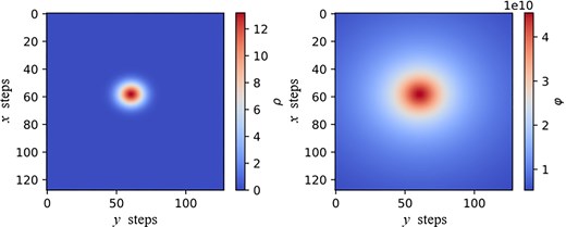
(Left) Spherically symmetric Gaussian distribution given by Eq. (31). (Right) The corresponding analytical potential field, sliced at |$z$| = 0.5 m.
In order to compare the numerical results of the TDM method with the analytical results, for the numerical calculation, we use the Dirichlet boundary condition to approximately represent the open boundary condition by the analytical potential distribution on the boundaries. By doing this, we avoid the electric field distortion caused by the approximation of the boundary conditions.
The potential of the 3D Gaussian density distribution with the Dirichlet boundary condition has been calculated and shown in Fig. 10, compared with the analytical solutions of Eq. (31). The deviation shown in the right panel of Fig. 10 is the difference between the numerical solution and the analytical solution, normalized by the maximum of the analytical potential field. It can be seen that the numerical solutions obtained from the TDM are in good agreement with the analytical solutions.
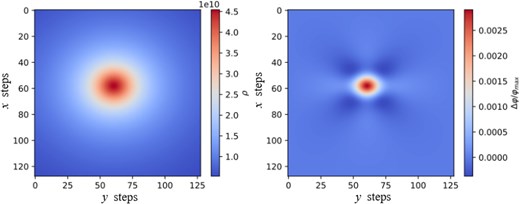
(Left) Numerical potential field obtained via the TDM algorithm. (Right) The deviation between the numerical solution and the analytical solution for comparison. Sliced at |$z=0.5$| m.
The major source of the error is due to the fact that the Dirichlet boundary has been defined as |$\varphi \ne 0$|, which is in disagreement with the basis |$U_X$| from Eq. (17) defined by |$\varphi = 0$| (odd distribution) near the boundaries. Other contributions to the error may arise from the choice of the numerical scheme and the grid resolution.
5.2. 2D beam of arbitrary distribution with open boundary
For more realistic particle distributions, the analytical solution of the Poisson equation is not available. We use the CIC method to obtain the charge density on the 2D grid from 200k macro particles with a given distribution. Figure 11 shows the charge distribution and the corresponding numerical potential field obtained via the widely employed FFT method based on Green’s function [12]. The potential field obtained via the TDM algorithm and the deviation from the FFT result are shown in Fig. 12. One can see that the two algorithms are in good agreement. The difference between the two methods is less than |$2\%$|.
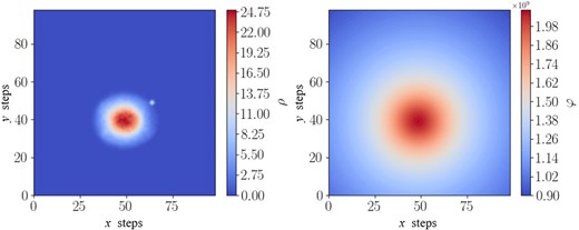
(Left) Example of 2D arbitrary distribution. (Right) The corresponding numerical potential field obtained via the FFT method.

(Left) The numerical potential field obtained via the TDM algorithm. (Right) The deviation between the solutions via the TDM algorithm and via the FFT method, for comparison.
5.3. 3D cylindrical bunch with transverse round boundary and longitudinal open boundary
To verify the validity of Eq. (30) under the conditions of a nonrectangular beam pipe, let us consider a cylindrical bunch with transverse Gaussian distribution and longitudinal uniform distribution. Such a bunch is demonstrated with five slices in the upper panel of Fig. 13. The density function of the bunch |$\rho (r, z)$| can be written as
in which |$r= \sqrt{x^2+y^2}$| is the transverse displacement, |$Q$| the total charge of the bunch, |$\sigma$| the transverse rms beam size, and |$l$| the longitudinal beam length. |${\mathrm{ H}(z)}$| represents the Heaviside function. In the instance shown in Fig. 13, we choose |$\sigma = 0.015$| m, |$l = 1.0$| m, and the beam pipe radius is 0.1 m. The steps of the 3D grids are chosen as |$N_x = 63$|, |$N_y = 63$|, |$N_z = 123$|.
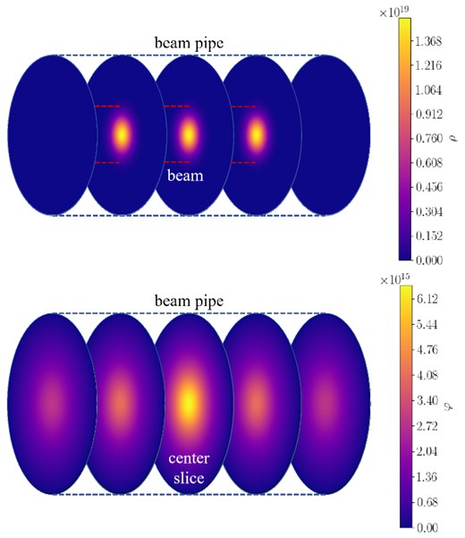
(Upper) The charge density on five representative evenly distributed longitudinal slices of the 3D cylinder beam. The red dashed lines represent the transverse beam size at 5|$\sigma$|. The round beam pipe is also shown as blue dashed lines. (Lower) The numerical results of the potential field on the five longitudinal slices of the beam calculated via the TDM algorithm.
The potential field of the cylindrical bunch with the round beam pipe is calculated via Eq. (30), and the result is shown in the lower panel of Fig. 13. One can see that the potential field reaches its maximum at the center of the bunch, and reduces down to 0 on the surface of the beam pipe wall.
On the other hand, the 2D transverse electric field of a transverse Gaussian distribution for a coasting beam with a round beam pipe can be analytically written as (here, the potential on the round beam pipe is set to zero):
where |$\lambda$| denotes the line density, which is a constant for the coasting beam. In order to compare with the numerical results of the cylindrical bunch in Fig. 13, we set |$\lambda = Q/l$|, and |$\sigma = 0.015$| m in Eq. (34).
The comparison of 2D electric fields in the center slice of the cylindrical bunch (marked as “center slice” in the lower panel of Fig. 13) and the electric fields of the coasting beam is shown in Fig. 14. It can be seen that the numerical solution of the discrete Poisson equation in Eq. (30) is in good agreement with the 2D analytical solution of Eq. (34).

Comparison of the 2D analytical solution |$E_r$| (red dots) and the center slice of the 3D numerical solution (blue line).
The model of the 2D coasting beam is widely employed for the study of beam dynamics, under the assumption of the realistic finite bunch length as infinite. The major advantage of the model is the 3D beam dynamics can be decoupled and dealt with in the 2D and the 1D domain, respectively. An interesting question may be raised as to what extent the 3D cylindrical bunch can be well represented by the 2D coasting beam model. The numerical calculation based on Eq. (30) can be applied to address this issue. Specifically, the comparison of the 3D cylindrical beam and the 2D coasting beam with varying longitudinal bunch length is shown in Fig. 15. One can observe that when |$l \gg \sigma$| (which is typical for hadron synchrotrons), the electric field on the the center slice of the 3D cylindrical beam trends to the 2D analytical result.
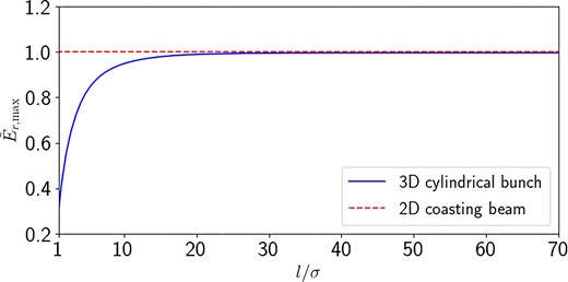
The maximum transverse electric field |$\tilde{E}_{r, \mathrm{max}}$| of the 3D cylindrical bunch model (normalized to the maximum transverse electric field of the 2D coasting beam model) as a function of the longitudinal beam length |$l$| normalized to the transverse rms beam size |$\sigma = 0.015$| m. The beam pipe radius is 0.1 m.
6. Conclusion
In summary, we have developed the 3D space charge solver based on the tensor decomposition of discretized charge distribution. In this method, various typical boundary conditions can be taken into account. It is shown that with the adoption of the tensor representation, the computational cost of the proposed method can be much reduced by using the |$n$|-mode product.
The benchmarking with the analytical solution of a typical 3D distribution and the numerical solution of an arbitrary 2D distribution shows that the proposed TDM gives numerical solutions of the Poisson equation with high accuracy for specified boundary conditions.
With the advantage of the inclusion of flexible boundary conditions, we believe that TDM warrants consideration as a viable alternative to the existing methodologies. For example, one potential application is for the 3D electron bunch with high luminosity and low emittance. Another important application of the TDM is for the beam-beam effect calculation, which is being developed.
Acknowledgements
The authors would like to thank Prof. Kazuhito Ohmi and Ji Qiang for valuable discussions and suggestions.
Funding
This work is jointly supported by the National Natural Science Foundation of China (Grant No. 12475155), the GuangDong Basic and Applied Basic Research Foundation (Project Nos. 2024A1515012658), and the International Partnership Program of Chinese Academy of Sciences (Grant No. 013GJHZ2023026FN).
Data availability
Data will be made available on request.
Appendix A. The n-mode product
The |$n$|-mode product is a fundamental operation in the realm of tensor calculus, and plays a pivotal role in multidimensional data analysis and TDMs. It extends the concept of matrix multiplication to higher-order tensors. It is denoted as |$ \mathcal {X} \times _n A$|, where |$ \mathcal {X}$| is a tensor, |$ A$| is a matrix, and |$n$| denotes a certain mode (dimension) along which the |$n$|-mode product is conducted.
To elucidate the concept of the |$n$|-mode product, consider a third tensor |$ \mathcal {X}$| of size |$ I \times J \times K$| and three matrices |$A$|, |$B$|, and |$C$| of size |$ I \times L$|, |$ J \times M$|, and |$ K \times N$|, respectively. The |$n$|-mode product of |$ \mathcal {X}$| by |$ \mathbf {A}$| along its first mode (i.e. |$ n = 1$|) results in a new tensor of size |$ L \times J \times K$|. The operation is defined as
where |$ a_{li}$|, |$ b_{mj}$|, and |$ c_{nk}$| are the elements of matrix |$A$|, |$B$|, and |$C$|, respectively, and |$ x_{ijk}$| are the elements of the tensor |$ \mathcal {X}$|. Similarly, the discretized Poisson equation in Eq. (5) can be rewritten as
Appendix B. Location choice of data points
In Fig. 1, |$\mathrm{ f}(X_i)$| is a first-order approximation of the integral from |$ X_i - \frac{h_X}{2}$| to |$ X_i + \frac{h_X}{2}$|, given as
It can be seen from Eq. (B1) that the sum of all data points approximates the integral from 0 to |$ L_X$|.
On the other aspect, let us consider that the data points are located at the grid boundaries. In this case, the sum of all data points is dependent on the integral over the interval |$ -\frac{h_X}{2}$| to |$ L_X + \frac{h_X}{2}$|, which introduces a bias. This error becomes more obvious with fewer discrete data points. Similarly, the inner products between the data point vectors and the basis vectors, as well as the inner products among basis vectors, would correspond to the integral over |$ -\frac{h_X}{2}$| to |$ L + \frac{h_X}{2}$| rather than 0 to |$L$|, i.e.
in which |$F_X$| and |$G_X$| are, respectively, the discretized form of |$\mathrm{ f}(x)$| and |$\mathrm{ g}(x)$| with the points located on the grid boundaries. For certain basis functions, such as Legendre polynomials, which are orthogonal over the interval |$[-1, 1]$|, extending the integration range would cause loss of orthogonality and a reduction in the accuracy of the numerical solution.
References
Author notes
These authors contributed equally to this work.
