


Abstract
We study the thermodynamics and thermodynamic geometry of the (2+1)D Banados–Teitelboim–Zanelli (BTZ) black hole within the framework of the nonextensive generalizations of Gibbs entropy. We investigate both the rotating (R-BTZ) and the charged (C-BTZ) BTZ black holes in these nonextensive entropy formalisms. We write down the Bekenstein–Hawking (BH) entropy of the black hole in terms of the nonextensive entropies, namely Kaniadakis entropy, Renyi entropy, and Barrow entropy. We investigate their impact on the thermodynamic phase structure and geometry of the BTZ black holes in both the ensembles, i.e. the fixed |$(J)$| and fixed |$(\Omega )$| ensembles for the R-BTZ black hole and the fixed |$(Q)$| and fixed |$(\Phi )$| ensembles for the C-BTZ black hole, where |$J$|, |$\Omega$|, |$Q$|, and |$\Phi$| represent the angular momentum, angular velocity, charge, and the electric potential of the respective black holes. We investigate the Ruppeiner and geometrothermodynamic (GTD) geometries of the black hole for all the nonextensive entropy cases. We find that there are both Davies-type and Hawking–Page phase transitions in both the charged and rotating BTZ black holes for the Kaniadakis entropy case in all the above-mentioned thermodynamic ensembles. These phase transitions were not seen in the BH entropy case. We also find that the Ruppeiner and the GTD scalar for the Kaniadakis entropy show curvature singularities corresponding to Davies-type phase transitions in both the rotating and charged BTZ black holes.
1. Introduction
It is by now well known that black holes are thermodynamic objects characterized by a temperature (Hawking temperature) proportional to the surface gravity at the horizon and entropy (Bekenstein–Hawking, BH, entropy) proportional to the horizon area [1,2]:
These two quantities (|$T$| and |$S_\mathrm{BH}$|) constitute the basis of what is now known as black hole thermodynamics [3]. Over the years, black hole thermodynamics has evolved into an active area of research with a number of generalizations of its original version [4–9] shedding light on the phase structures of black holes.
An important issue in the context of black hole thermodynamics that has recently come into focus is the modification of black hole entropy owing to different corrections. These corrections result in a number of nonextensive generalizations of Gibbs entropy. Some of these notable entropies are: Kaniadakis entropy [10,11], Renyi entropy [12], and Barrow entropy [13]. A brief introduction to these entropies will be provided in the next section. The impact of these entropies on the thermodynamic behavior of a few black holes has been studied in a number of works [14–18]. Previously these entropy systems have been tested in cosmology [19–23] and quantum physics [24–28] with notable success.
Although we employ Kaniadakis, Renyi, and Barrow entropies individually for our convenience here, it is worth noting that generalized entropy constructs with different parameters have been introduced in Refs. [22,23] that generalize all the above-mentioned entropies. These generalized entropy constructs are formulated such that they reduce to all the required entropy paradigms under appropriate limits. For example, the six-parameter entropy formulation proposed in Ref. [23] is given as:
where all parameters |$(\alpha _{\pm }, \beta _{\pm }, \gamma _{\pm })$| are positive. This expression reduces to the above-mentioned entropy formulations under specific parameter limits, as outlined below:
- Kaniadakis entropy: By taking |$\beta _{\pm } \rightarrow 0$|, |$\gamma _{\pm } = 1$|, and |$\alpha _{\pm } = K$|, the generalized entropy simplifies to(3)$$\begin{eqnarray} S_G \rightarrow \frac{1}{K} \sinh (KS), \end{eqnarray}$$
which corresponds to the Kaniadakis entropy.
- Renyi entropy: From the Sharma–Mittal limit, if |$\alpha _{+} \rightarrow 0$|, |$\beta _{+} \rightarrow 0$|, and |$\alpha _{+}/\beta _{+} \rightarrow \alpha$|, with |$\gamma _{+} = 1$|, we recover the Renyi entropy:(4)$$\begin{eqnarray} S_G \rightarrow \frac{1}{\alpha } \ln (1 + \alpha S). \end{eqnarray}$$
- Sharma–Mittal entropy: Setting |$\alpha _{-} = 0$| and |$\gamma _{+} = 1$|, we obtain(5)$$\begin{eqnarray} S_G = \frac{1}{\alpha _{+}} \left[ \left( 1 + \frac{\alpha _{+}}{\beta _{+}} S^{\gamma _{+}} \right)^{\beta _{+}} - 1 \right]. \end{eqnarray}$$
Choosing |$\alpha _{+} = R$|, |$\beta _{+} = R/\delta$|, and |$\gamma _{+} = \delta$|, the Sharma–Mittal entropy is reproduced.
Tsallis and Barrow entropy: In the limit |$\alpha _{+} = \alpha _{-} \rightarrow 0$| and |$\gamma _{+} = \gamma _{-} = \gamma$|, the generalized entropy reduces to |$S_G \rightarrow S^{\gamma }$|. By further choosing |$\gamma = \delta$| or |$\gamma = 1 + \Delta /2$|, we recover the Tsallis entropy and Barrow entropy, respectively.
- Loop quantum gravity entropy: Setting |$\alpha _{-} = 0$| and |$\gamma _{+} = 1$|, the entropy becomes(6)$$\begin{eqnarray} S_G = \frac{1}{\alpha _{+}} [ e^{\beta _{+} S} - 1]. \end{eqnarray}$$In the limit |$\beta _{+} \rightarrow \infty$| and |$\alpha _{+} = 1 - q$|, this reduces to the loop quantum gravity entropy(7)$$\begin{eqnarray} S_G \approx \frac{1}{1 - q} [ e^{(1-q)S} - 1], \end{eqnarray}$$
which approaches the BH entropy as |$q \rightarrow 1$|.
The entropy |$S_G$| defined above does satisfy the generalized third law of thermodynamics and is seen to vanish when |$S \rightarrow 0$|. |$S_G$| is found to be a monotonically increasing function of |$S$|, thus reducing to the BH entropy under suitable limits.
Although black hole thermodynamics in its different forms has largely been successful in providing deep insights about the thermodynamic properties of black holes, there are a number of important issues that are far from being completely understood. One such issue is the microscopic origin of BH entropy. In the absence of a complete theory of quantum gravity, thermodynamic geometry studies of black holes have been used to extract qualitative ideas about microscopic interaction in black holes [29–31]. Thermodynamic geometry is a key concept in the study of black holes as they provide an understanding of the phase transitions in terms of the curvature singularities obtained through a particular thermodynamic metric. Three such metrics that have been used in black hole thermodynamics are the Weinhold, Ruppeiner, and geometrothermodynamic (GTD) metrics.
Weinhold [32] introduced a Riemannian metric in the equilibrium space, which is defined as the second derivative of the internal energy with respect to other extensive variables. The Weinhold metric is defined as:
where the internal energy |$U(S,X)$| is a function of entropy S and other extensive variables X.
Ruppeiner [33] later introduced a Riemannian metric that is defined as the negative Hessian of the entropy with respect to the other extensive variables. The Ruppeiner metric is a concept based on the thermodynamic fluctuation theory of equilibrium thermodynamics, where the thermodynamic length is related to the probability of fluctuation between two states of the thermodynamic system [34]. The two are inversely related as an increase in the probability of fluctuation would mean a significant decrease in the thermodynamic length and vice versa. The Ruppeiner metric is defined as:
where the entropy |$S(U,X)$| is a function of internal energy |$U$| and other extensive variables X. The Riemannian scalar that is defined here as |$R_\mathrm{Rupp}$| is a scalar invariant function in thermodynamic geometry. The sign of the scalar curvature has been linked to the nature of microscopic interactions in the thermodynamic system. For positive or negative scalar curvatures, the underlying interaction is either repulsive or attractive accordingly, whereas a null curvature would mean an absence of interaction with a flat thermodynamic geometry. The Ruppeiner and the Weinhold metrics are conformally related to each other by the following relation [35,36]:
where |$T=\frac{\partial {U}}{\partial {S}}$| is the Hawking temperature of the system with |$U^i =(U,X)$| and |$S^i =(S,X)$|.
The Ruppeiner and Weinhold geometries have successfully predicted the occurrence of phase transitions in the case of ordinary thermodynamic systems. However, contradictory results are seen for black holes, where, for instance, in a Kerr black hole [37] the Weinhold metric showed no phase transition, whereas the Ruppeiner metric could show phase transitions only for a specific thermodynamic potential. However, such problems were successfully addressed in the new geometric formalism of GTD [38] where the properties of the phase space and the space of equilibrium states could be unified [39]. The GTD metric is a Legendre invariant metric and therefore would not depend on any specific choice of thermodynamic potential. The phase transitions obtained from the specific heat capacity of the black hole are properly contained in the scalar curvature of the GTD metric, such that a curvature singularity in the GTD scalar |$R_\mathrm{GTD}$| would imply the occurrence of a phase transition. The general form of the GTD metric is given by [40]:
where |$\varphi$| is the thermodynamic potential and |$E^a$| is an extensive thermodynamic variable with |$a=1,2,3....$|.
In this paper, we study the thermodynamics and thermodynamic geometry of the (2+1)D Banados–Teitelboim–Zanelli (BTZ) black hole within the framework of the nonextensive generalizations of Gibbs entropy. We investigate both the rotating (R-BTZ) and the charged (C-BTZ) BTZ black holes in these nonextensive entropy formalisms. We write down the BH entropy of the black hole in terms of the nonextensive entropies, namely Kaniadakis entropy, Renyi entropy, and Barrow entropy. We investigate their impact on the thermodynamic phase structure and geometry of the BTZ black hole in both the ensembles, i.e. the fixed |$(J)$| and fixed |$(\Omega )$| ensembles for the R-BTZ black hole and the fixed |$(Q)$| and fixed |$(\Phi )$| ensembles for the C-BTZ black hole, where |$ J$|, |$\Omega$|, |$Q$|, and |$\Phi$| represent the angular momentum, angular velocity, charge, and the electric potential of the respective black holes. We investigate the Ruppeiner and GTD geometries of the black hole for all the nonextensive entropy cases.
In this study, we adopt the energy definition of General Relativity, the first law of thermodynamics, and the conventional definition of thermodynamic temperature as fundamental. However, we accept the alternative viewpoint that has been adopted in Refs. [24,25] based on the assumption that the Hawking temperature must be kept unaffected. Furthermore, it has been demonstrated that nonextensive entropy paradigms can lead to wrong expressions for the Hawking temperature or black hole energy that differ from the standard ones. While we acknowledge these critiques, we argue that any modification to these quantities such as the Hawking temperature under these nonextensive entropy formalisms should be interpreted as a shift in the effective thermodynamic description rather than a fundamental change to the Hawking temperature itself. These effective temperatures reflect the corrections introduced by nonextensive statistical mechanics and are not meant to replace the fundamental Hawking temperature. The effective temperatures characterize the modified thermodynamic equilibrium within each of the nonextensive paradigms and provide insights into how such generalizations affect black hole systems. These differences highlight the speculative yet potentially valuable role of nonextensive frameworks in exploring new physical scenarios and enriching our understanding of black hole thermodynamics. We stress the fact that the exploration of different nonextensive entropies is motivated by their success in describing physical systems beyond black holes [41–46]. The study of their implications for black hole thermodynamics provides us with an opportunity to test the limits of our current understanding and to further explore potential extensions of the standard approach.
The paper is structured as follows. In Section 2 we review some known facts about the nonextensive generalizations of Gibbs entropy. Section 3 is about the rotating BTZ black hole and its thermodynamic investigation within the framework of nonextensive entropies in two different ensembles. In Section 4 we examine the thermodynamic geometry of the black hole system in both the Ruppeiner and GTD formalisms. Section 5 is about the thermodynamic investigation of the charged BTZ black hole within the framework of nonextensive entropies in two different ensembles. In Section 6 we examine the thermodynamic geometry of the black hole in both the Ruppeiner and GTD formalisms. The final section contains our conclusions.
2. Nonextensive generalizations of Gibbs entropy
The entropy of a black hole scales with its area rather than its volume and is therefore regarded as a nonextensive quantity. Due to its nonextensive nature, the black hole entropy is also nonadditive and follows a nonadditive composition rule. But in the case of Gibbs thermodynamics the entropy is defined to be both extensive and additive as it scales with the size of the system. However, the assumption of extensivity of Gibbs entropy is due to ignoring the long-range forces that are prevalent between thermodynamic subsystems. Gibbs thermodynamics ignores these forces because the size of the system exceeds the interaction range between the thermodynamic subsystems. The total entropy thus becomes equal to the sum of the entropies of its components. It therefore grows with the size of the thermodynamic system.
But these long-range forces are important in various thermodynamic systems such as black holes. We can therefore infer that Gibbs thermodynamics may not be a suitable choice for studying black hole thermodynamics. Therefore, in order to understand the nonextensive nature of black hole entropy, several nonextensive generalizations of Gibbs entropy have been prescribed. We give a brief outline of a few of those entropies in the following subsections, which we will use later in order to study the thermodynamics and thermodynamic geometry of both the rotating and charged BTZ black holes respectively.
2.1. Kaniadakis entropy
Kaniadakis entropy [10,11,14,47–50] is a relativistic nonextensive generalization of Boltzmann–Gibbs entropy. It was proposed by Kaniadakis so as to accommodate special relativity with nonextensive statistical mechanics. Kaniadakis entropy is premised upon the fact that physical observables such as momentum and energy when generalized under special relativity are viewed as a one-parameter deformation of the corresponding nonrelativistic formula, i.e. |$P^{\prime } =\frac{P}{\sqrt{1- x^2}}$|, where |$P^{\prime }$| is the relativistic momentum and |$x=\frac{v}{c}$| is the deformation parameter. It is therefore quite obvious that the entropy of a relativistic system could also be seen as a one-parameter deformation of the classical nonrelativistic entropy. In order to achieve a relativistic formula for Boltzmann–Gibbs entropy, Kaniadakis proposed a deformed logarithmic function in the entropy formula, which in turn deforms the Maxwell–Boltzmann distribution function. These deformed functions are given as:
where x is a variable and K is the deformation parameter called the Kaniadakis parameter; both of the above-mentioned deformed functions reduce to their original form as the deformed parameter K approaches the appropriate limit, i.e. |$K \rightarrow 0$|. The Kaniadakis entropy is then defined as:
where
In the limit |$K \rightarrow 0$|, the Kaniadakis entropy reduces to the Boltzmann–Gibbs entropy. Considering the equiprobability of microstates inside the black hole we can reduce the Kaniadakis entropy to:
where |$n$| is the number of microstates of the thermodynamic system and K is the Kaniadakis parameter. On further simplification we obtain:
Considering that the BH entropy is obtained by counting the number of microstates inside the black hole as shown by Strominger and Vafa in their seminal work [51], we write the BH entropy |$S_\mathrm{BH}=\ln (n)$| such that the above equation reduces to:
where, for the limit |$K \rightarrow 0$|, SK → SBH.
2.2. Renyi entropy
The Renyi entropy [52–58] is a nonextensive generalization of Boltzmann–Gibbs entropy where, unlike the case where all the probabilities are treated uniformly, Renyi entropy allows for a parameter adjustment to the sensitivities of different probabilities in the system. This becomes very useful in situations where either rare or highly probable events demand separate emphasis. The Renyi entropy is a measure of the quantum entanglement of a system, a phenomenon where the quantum states of two or more particles could become correlated. It is defined as:
where P(i) is the probability distribution and q is the nonextensive Tsallis parameter. We here assume that the black hole entropy is just the Tsallis entropy [59–61], which is a one-parameter generalization of Boltzmann–Gibbs entropy so as to include both extensive and nonextensive statistical systems. The Tsallis entropy is given by:
where, for |$q \rightarrow 1$|, |$S_T$| reduces to the usual Boltzmann–Gibbs entropy. The parameter |$ q$| is responsible for the degree of nonextensivity of the entropy:
For |$ q = 1$|: Tsallis entropy reduces to the extensive Boltzmann–Gibbs entropy, which is appropriate for a system that comprises weak correlations and short-range interactions.
For |$ q \lt 1$|: The entropy is subextensive and is useful in describing systems where the probability for the occurrence of rare states is higher than the occurence of frequent states.
For |$ q \gt 1$|: The entropy shows superextensive behavior where frequent states contribute more to the entropy.
By performing the necessary substitutions, the Renyi entropy can be defined as follows:
and, after putting |$1-q =\lambda$|, we get the Renyi entropy in terms of BH entropy as:
where |$\lambda$| is the Renyi parameter and, for the limit |$\lambda \rightarrow 0$|, SR → SBH.
2.3. Barrow entropy
The Barrow entropy [13,62,63], introduced by John Barrow, is proposed to measure the entropy of a black hole system whose smooth horizon has been replaced by rough fractal structures. Unlike the above two entropy formalisms, Barrow entropy does not have a statistical root. It is a modification introduced in the context of quantum gravity and the fractal structure of space-time. It is formulated by considering quantum-gravitational effects that modify the surface of the black hole’s event horizon by considering the structure of the horizon to be fractal-like. John Barrow’s approach to entropy suggests that the horizon area might have a fractal dimension, which alters the traditional BH entropy formula. This modification puts forth a parameter that can quantify the degree of deviation from the standard horizon geometry due to quantum corrections while capturing the complexity of space-time at smaller scales. The Barrow entropy is formulated as:
where |$\Delta$| is the Barrow parameter that is linked to the fractal structure of the system with range |$0\lt \Delta \le 2$|, where |$\Delta \rightarrow 2$| would yield maximal fractal structure and, for the limit |$\Delta \rightarrow 0$|, SΔ → SBH.
3. Thermodynamics of the rotating BTZ black hole
The action that facilitates the field equations [64–69] from which the |$(2+1)$|D rotating BTZ black hole solutions are obtained is given as:
where the anti-de Sitter (AdS) length |$l$| is related to the cosmological constant |$\Lambda$| by the relation |$\Lambda =- \frac{1}{l^2}$| and Einstein’s field equations are given by:
The line element that corresponds to the given solution is:
where |$f(r) = -M + \frac{r^2}{l^2} + \frac{J^2}{4 r^2}$| and M and J are the mass and angular momentum carried by the black hole. Solving the function for |$f(r)=0$| would give us the roots that determine the horizon radius. For an exterior horizon radius |$r_{+}$|, the black hole mass is given by:
and the black hole entropy is given by:
3.1. The Kaniadakis entropy case
The Kaniadakis entropy |$S_K$| in terms of the black hole entropy |$S_\mathrm{BH}$| is given by Eq. (10) as:
where K is the Kaniadakis parameter and, for |$K \rightarrow 0$|, SK → SBH. Starting with the above equation we get the modified horizon radius for the R-BTZ black hole as:
Fixed |$(J)$| ensemble:
We replace the horizon radius in Eq. (13) by the one obtained in Eq. (14) to get the modified mass |$M_{K}$| for the R-BTZ black hole, given by:
The function |$\mathrm{\mathrm{arcsinh}}[K S_{K}]$| can be replaced by its logarithmic form |$\ln \big[KS_{K}+ \sqrt{1 + K^2 S_{K} ^2}\big]$| and therefore the expression for mass becomes:
The heat capacity for the Kaniadakis entropy case in the fixed |$(J)$| ensemble can be obtained as:
where
and
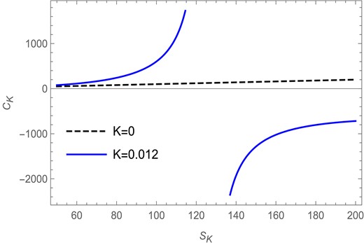
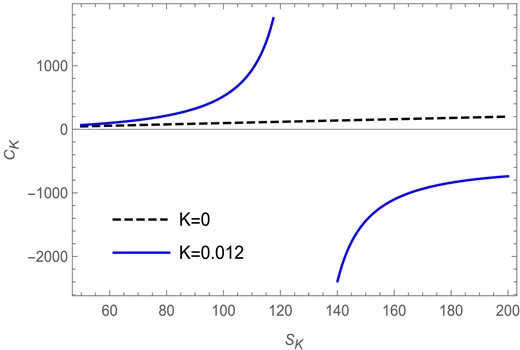
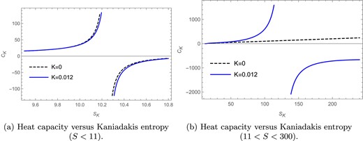
In Fig. 1 the heat capacity |$C_K$| is plotted against the Kaniadakis entropy |$S_K$| for |$l=1$| and |$J=1$| in the fixed |$(J)$| ensemble. Here the solid blue curve represents the heat capacity for the Kaniadakis parameter |$K=0.012$|, whereas the black dashed line represents the heat capacity for the BH entropy case |$(K=0)$|. We find that, for |$K=0.012$|, the heat capacity has a divergence at |$S_K=125.77$|, which indicates the presence of a Davies-type phase transition in the Kaniadakis modified black hole, whereas the heat capacity for the BH entropy case shows no such behavior.
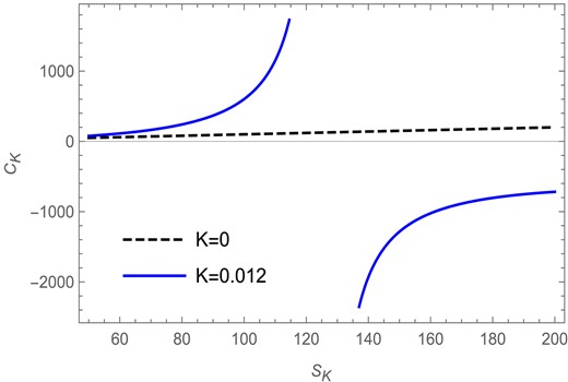
The heat capacity versus Kaniadakis entropy plot in the fixed |$(J)$| ensemble for |$l=1$| and |$J=1$|.
The Gibbs free energy for the Kaniadakis entropy case in the fixed |$(J)$| ensemble can be obtained as:
where
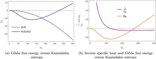
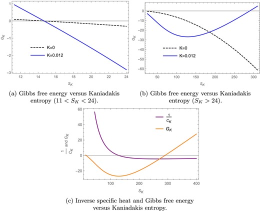
In Figs. 2(a) and (b) the Gibbs free energy |$G_K$| is plotted against the Kaniadakis entropy |$S_K$| for |$l=1$| and |$J=1$| in the fixed |$(J)$| ensemble. We draw two different plots so as to make the presence of the phase transitions more transparent. Here the solid blue curve represents the Gibbs free energy for the Kaniadakis parameter |$K=0.012$|, whereas the black dashed line represents the free energy for the BH entropy case |$(K=0)$|. The free energy for the |$K=0$| case has been scaled down by multiplying it by |$\frac{1}{10}$|, whereas the free energy for the |$K=0.012$| case is kept the same; this difference in scaling is just so that the distinct behavior of both the curves can be seen more clearly. We keep in mind that the scaling does not affect the position or occurrence of the phase transitions. We find that in Fig. 2(a) the Gibbs free energy goes to zero for both the entropy cases, where, for |$K=0$|, the zero point is at |$S_K =11.69$| and, for |$K=0.012$|, the zero point is found to be at |$S_K =11.75$|; these zero points refer to the presence of a Hawking–Page phase transition in the rotating BTZ black hole for both the BH as well as the Kaniadakis entropy cases. We again find that, for |$K=0.012$|, the Gibbs free energy in Fig. 2(b) has a zero point at |$S_K=276.64$| only for the Kaniadakis entropy case, which indicates the presence of a Hawking–Page phase transition in the Kaniadakis modified black hole, whereas the Gibbs free energy for the BH entropy case shows no such behavior. In Fig. 2(c) we plot the inverse of specific heat capacity (purple) and the Gibbs free energy (orange) against the Kaniadakis entropy. The inverse of specific heat capacity has been scaled up by multiplying it by 3000, whereas the free energy is kept the same; this difference in scaling is just so that the distinct behavior of both the curves can be seen more clearly. We keep in mind that the scaling does not affect the position or occurrence of the phase transitions. The points where these curves intersect the horizontal axis represent the Davies-type (purple) and Hawking–Page (orange) phase transitions respectively, which are seen to be quite distant from each other.
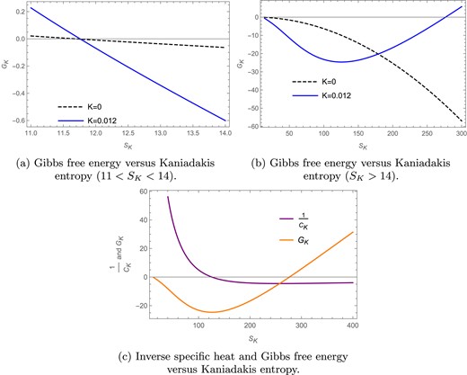
The Gibbs free energy curves for Kaniadakis entropy in the fixed |$(J)$| ensemble for |$l=1$| and |$J=1$|.
Fixed |$(\Omega )$| ensemble:
The modified mass for the Kaniadakis entropy case in the fixed |$(\Omega )$| ensemble is given by:
where |$\frac{\partial M_{K}}{\partial J}= \Omega$| is the angular velocity of the black hole with respect to the angular momentum J. By writing the term |$M_{K} ^{\prime }$| as |$M_{K}$| for convenience we get:
The heat capacity for the Kaniadakis entropy case in the fixed |$(\Omega )$| ensemble can be obtained as:
The heat capacity of the rotating BTZ black hole is independent of |$\Omega$| as can be seen from the above expression and therefore the presence or absence of Davies-type phase transitions in the fixed |$(\Omega )$| ensemble is independent of |$\Omega$|. In Fig. 3 the heat capacity |$C_K$| is plotted against the Kaniadakis entropy |$S_K$| for |$l=1$| in the fixed |$(\Omega )$| ensemble. Here the solid blue curve represents the heat capacity for the Kaniadakis parameter |$K=0.012$|, whereas the black dashed line represents the heat capacity for the BH entropy case |$(K=0)$|. We find that, for |$K=0.012$|, the heat capacity has a divergence at |$S_K=125.74$|, which indicates the presence of a Davies-type phase transition in the Kaniadakis modified black hole, whereas the heat capacity for the BH entropy case shows no such behavior.
The heat capacity versus Kaniadakis entropy plot in the fixed |$(\Omega )$| ensemble for |$l=1$| and |$\Omega =0.2$|.
The Gibbs free energy for the Kaniadakis entropy case in the fixed |$(\Omega )$| ensemble can be obtained as:
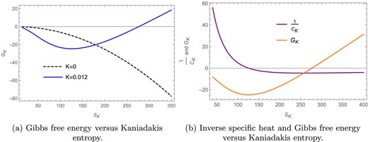
In Fig. 4(a) the Gibbs free energy |$G_K$| is plotted against the Kaniadakis entropy |$S_K$| for |$l=1$| and |$\Omega =0.2$| in the fixed |$(\Omega )$| ensemble. Here the solid blue curve represents the Gibbs free energy for the Kaniadakis parameter |$K=0.012$|, whereas the black dashed line represents the free energy for the BH entropy case |$(K=0)$|. The free energy for the |$K=0$| case has been scaled down by multiplying it by |$\frac{1}{10}$|, whereas the free energy for the |$K=0.012$| case is kept the same; this difference in scaling is just so that the distinct behavior of both the curves can be seen more clearly. We keep in mind that the scaling does not affect the position or occurrence of the phase transition. We find that, for |$K=0.012$|, the Gibbs free energy has a zero point at |$S_K=276.65$|, which indicates the presence of a Hawking–Page phase transition in the Kaniadakis modified black hole, whereas the Gibbs free energy for the BH entropy case shows no such behavior. In Fig. 4(c) we plot the inverse of specific heat capacity (purple) and the Gibbs free energy (orange) against the Kaniadakis entropy. The inverse of specific heat capacity has been scaled up by multiplying it by 3000, whereas the free energy is kept the same; this difference in scaling is just so that the distinct behavior of both the curves can be seen more clearly. We keep in mind that the scaling does not affect the position or occurrence of the phase transitions. The points where these curves intersect the horizontal axis represent the Davies-type (purple) and Hawking–Page (orange) phase transitions respectively, which are seen to be quite distant from each other.
The Gibbs free energy curves for Kaniadakis entropy in the fixed |$(\Omega )$| ensemble for |$l=1$| and |$\Omega =0.2$|.
3.2. The Renyi entropy case
The Renyi entropy |$S_R$| in terms of the black hole entropy |$S_\mathrm{BH}$| is given by Eq. (11) as:
where |$\lambda$| is the Renyi parameter and, for the limit |$\lambda \rightarrow 0$|, SR → SBH. Starting with the above equation we get the modified horizon radius for the R-BTZ black hole as:
Fixed |$(J)$| ensemble:
We replace the horizon radius in Eq. (13) by the one obtained in Eq. (23) to get the modified mass |$M_{R}$| for the R-BTZ black hole, given by:
The heat capacity for the Renyi entropy case in the fixed |$(J)$| ensemble can be calculated as:
where
and
We see from Fig. 5(a) that the heat capacity |$C_R$| for the rotating BTZ black hole is plotted against the Renyi entropy |$S_R$| in the fixed |$(J)$| ensemble. Here the solid green curve represents the heat capacity for the Renyi parameter |$\lambda =0.012$|, whereas the black dashed line represents the heat capacity for the BH entropy case |$(\lambda =0)$|. For the parameters |$l=1$| and |$ J=1$| we find that there are no divergences in the heat capacity curve for both the Renyi and BH entropy cases.
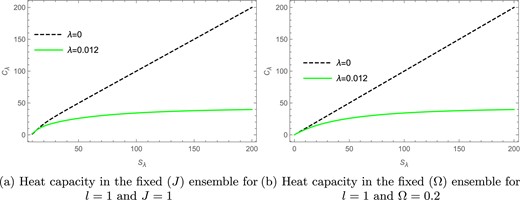
The heat capacity versus Renyi entropy plots in the fixed |$(J)$| and fixed |$(\Omega )$| ensembles.
The Gibbs free energy for the Renyi entropy case in the fixed |$(J)$| ensemble can be obtained as:
In Fig. 6(a) the Gibbs free energy |$G_R$| is plotted against the Renyi entropy |$S_R$| for |$l=1$| and |$J=1$| in the fixed |$(J)$| ensemble. Here the solid green curve represents the Gibbs free energy for the Renyi parameter |$\lambda =0.012$|, whereas the black dashed line represents the free energy for the BH entropy case |$(\lambda =0)$|. The free energy for the |$\lambda =0$| case has been scaled down by multiplying it by |$\frac{1}{10}$|, whereas the free energy for the |$\lambda =0.012$| case is kept the same; this difference in scaling is just so that the distinct behavior of both the curves can be seen more clearly. We find that in Fig. 6(a) the Gibbs free energy goes to zero for both the entropy cases, where, for |$\lambda =0$|, the zero point is at |$S_R =11.69$| and, for |$\lambda =0.012$|, the zero point is found to be at |$S_R =10.74$|; these zero points refer to the presence of a Hawking–Page phase transition in the rotating BTZ black hole for both the BH as well as the Renyi entropy cases.
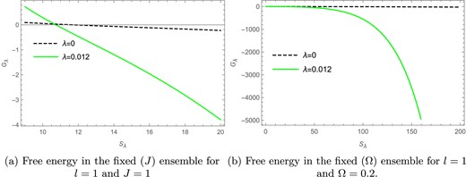
The Gibbs free energy versus Renyi entropy plots in the fixed |$(J)$| and fixed |$(\Omega )$| ensembles.
Fixed |$(\Omega )$| ensemble:
The modified mass for the Renyi entropy case in the fixed |$(\Omega )$| ensemble is given by:
where |$\frac{\partial M_{R}}{\partial J}= \Omega$| is the angular velocity of the black hole with respect to the angular momentum J. By making the necessary replacements and putting |$l=1$|, we get the final equation as follows:
We have here used the term |$M_{R}$| instead of |$M_{R}^{\prime }$| for convenience. Here |$M_{R}$| is the modified mass for the fixed |$(\Omega )$| ensemble. The heat capacity for the Renyi entropy case in the fixed |$(\Omega )$| ensemble can be calculated as:
The heat capacity of the rotating BTZ black hole is independent of |$\Omega$| as can be seen from the above expression and therefore the presence or absence of Davies-type phase transitions is independent of |$\Omega$|. We see from Fig. 5(b) that the heat capacity |$C_R$| for the rotating BTZ black hole is plotted against the Renyi entropy |$S_R$| in the fixed |$(\Omega )$| ensemble. Here the solid green curve represents the heat capacity for the Renyi parameter |$\lambda =0.012$|, whereas the black dashed line represents the heat capacity for the BH entropy case |$(\lambda =0)$|. We see that for |$l=1$| there are no divergences in the heat capacity curve for both the Renyi and BH entropy cases.
The Gibbs free energy for the Renyi entropy case in the fixed |$(\Omega )$| ensemble can be obtained as:
In Fig. 6(b) the Gibbs free energy |$G_R$| is plotted against the Renyi entropy |$S_R$| for |$l=1$| and |$\Omega =0.2$| in the fixed |$(\Omega )$| ensemble. Here the solid green curve represents the Gibbs free energy for the Renyi parameter |$\lambda =0.012$|, whereas the black dashed line represents the free energy for the BH entropy case |$(\lambda =0)$|. The free energy for the |$\lambda =0$| case has been scaled down by multiplying it by |$\frac{1}{10}$|, whereas the free energy for the |$\lambda =0.012$| case is kept the same; this difference in scaling is just so that the distinct behavior of both the curves can be seen more clearly. We find that, unlike the Kaniadakis entropy, there is no Hawking–Page phase transition present in the Renyi entropy case for the fixed |$(\Omega )$| ensemble.
3.3. The Barrow entropy case
The Barrow entropy |$S_{\Delta }$| in terms of the black hole entropy |$S_\mathrm{BH}$| is given by Eq. (12) as:
where |$\Delta$| is the parameter that is linked to the fractal structure of the system and, for the limit |$\Delta \rightarrow 0$|, SΔ → SBH. Starting with the above equation we get the modified horizon radius for the R-BTZ black hole as:
Fixed |$(J)$| ensemble:
We replace the horizon radius in Eq. (13) by the one obtained in Eq. (30) to get the modified mass |$M_{\Delta }$| for the R-BTZ black hole, given by:
The heat capacity for the Barrow entropy case in the fixed |$(J)$| ensemble can be calculated as:
We see from Fig. 7(a) that the heat capacity |$C_{\Delta }$| for the rotating BTZ black hole is plotted against the Barrow entropy |$S_{\Delta }$| in the fixed |$(J)$| ensemble. Here the solid red curve represents the heat capacity for the Barrow parameter |$\Delta =0.012$|, whereas the black dashed line represents the heat capacity for the BH entropy case |$(\Delta =0)$|. For the parameters |$l=1$| and |$ J=1$| we find that there are no divergences in the heat capacity curve for both the Barrow and BH entropy cases.
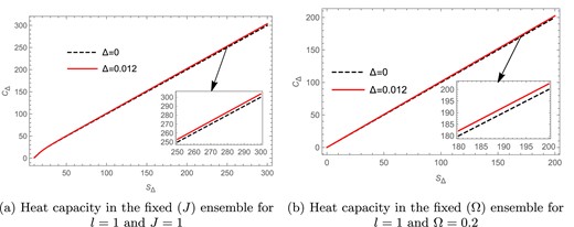
The heat capacity versus Barrow entropy plots in the fixed |$(J)$| and fixed |$(\Omega )$| ensembles.
The Gibbs free energy for the Renyi entropy case in the fixed |$(J)$| ensemble can be obtained as:
In Fig. 8(a) the Gibbs free energy |$G_\Delta$| is plotted against the Barrow entropy |$S_\Delta$| for |$l=1$| and |$J=1$| in the fixed |$(J)$| ensemble. Here the solid red curve represents the Gibbs free energy for the Barrow parameter |$\Delta =0.012$|, whereas the black dashed line represents the free energy for the BH entropy case |$(\Delta =0)$|. The free energy for the |$\Delta =0$| case has been scaled down by multiplying it by |$\frac{1}{10}$|, whereas the free energy for the |$\Delta =0.012$| case is kept the same; this difference in scaling is just so that the distinct behavior of both the curves can be seen more clearly. We find that in Fig. 8(a) the Gibbs free energy goes to zero for both the entropy cases, where, for |$\Delta =0$|, the zero point is at |$S_R =11.69$| and, for |$\Delta =0.012$|, the zero point is found to be at |$S_R =11.89$|; these zero points refer to the presence of a Hawking–Page phase transition in the rotating BTZ black hole for both the BH as well as the Barrow entropy cases.
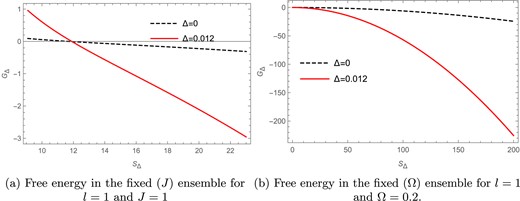
The Gibbs free energy versus Barrow entropy plots in the fixed |$(J)$| and fixed |$(\Omega )$| ensembles.
Fixed |$(\Omega )$| ensemble:
The modified mass for the Barrow entropy case in the fixed |$(\Omega )$| ensemble is given by:
where |$\frac{\partial M_{\Delta }}{\partial j}= \Omega$| is the angular velocity of the black hole with respect to the angular momentum J. By making the necessary replacements and putting |$l=1$|, we get the final equation as follows:
We have here used the term |$M_{\Delta }$| instead of |$M_{\Delta }^{\prime }$| for convenience. Here |$M_{\Delta }$| is the modified mass for the fixed |$(\Omega )$| ensemble. The heat capacity for the Barrow entropy case in the fixed |$(\Omega )$| ensemble can be calculated as:
The heat capacity of the rotating BTZ black hole is independent of |$\Omega$| as can be seen from the above expression and therefore the presence or absence of Davies-type phase transitions is independent of |$\Omega$|. We see from Fig. 7(b) that the heat capacity |$C_{\Delta }$| for the rotating BTZ black hole is plotted against the Barrow entropy |$S_{\Delta }$| in the fixed |$(\Omega )$| ensemble. Here the solid red curve represents the heat capacity for the Barrow parameter |$\Delta =0.012$|, whereas the black dashed line represents the free energy for the BH entropy case |$(\Delta =0)$|. We see that for |$l=1$| there are no divergences in the heat capacity curve for both the Barrow and BH entropy cases.
The Gibbs free energy for the Barrow entropy case in the fixed |$(\Omega )$| ensemble can be obtained as:
In Fig. 8(b) the Gibbs free energy |$G_\Delta$| is plotted against the Barrow entropy |$S_\Delta$| for |$l=1$| and |$\Omega =0.2$| in the fixed |$(\Omega )$| ensemble. Here the solid red curve represents the Gibbs free energy for the Renyi parameter |$\Delta =0.012$|, whereas the black dashed line represents the free energy for the BH entropy case |$(\Delta =0)$|. Here the solid red curve represents the Gibbs free energy for the Barrow parameter |$\Delta =0.012$|, whereas the black dashed line represents the free energy for the BH entropy case |$(\Delta =0)$|. The free energy for the |$\Delta =0$| case has been scaled down by multiplying it by |$\frac{1}{10}$|, whereas the free energy for the |$\Delta =0.012$| case is kept the same; this difference in scaling is just so that the distinct behavior of both the curves can be seen more clearly. We find that, unlike the Kaniadakis entropy, there is no Hawking–Page phase transition present in the Barrow entropy case for the fixed |$(\Omega )$| ensemble.
4. Thermodynamic geometry of the R-BTZ black hole
We discuss the thermodynamic geometry of the rotating BTZ black hole for both the Ruppeiner and GTD formalisms. The Ruppeiner metric is defined as the negative Hessian of entropy with respect to other extensive variables. Therefore it is only the fixed |$(J)$| ensemble that holds good in the Ruppeiner formalism as |$J$| is an extensive thermodynamic quantity, whereas |$\Omega$| is not.
Therefore the fixed |$(\Omega )$| ensemble does not hold good as per the definition of the Ruppeiner metric. We therefore discuss the thermodynamic geometry of the fixed |$(\Omega )$| ensemble in the GTD formalism, which is defined on a multidimensional phase space that comprises both the extensive and intensive variables of the thermodynamic system. The GTD formalism is therefore the appropriate geometric formalism for discussing both the thermodynamic ensembles.
We first discuss the Ruppeiner geometry of the rotating BTZ black hole in the fixed |$(J)$| ensemble where we observe a curvature singularity in the Ruppeiner scalar curve only for the Kaniadakis entropy case. We then discuss the GTD geometry of the black hole for both the thermodynamic ensembles, where we observe curvature singularities in the GTD scalar curves in the Kaniadakis entropy case only. These curvature singularities are seen to occur exactly at the points where we saw divergences in the corresponding heat capacity curves in the previous section.
4.1. Ruppeiner formalism
The Ruppeiner metric for the R-BTZ black hole in the fixed |$(J)$| ensemble can be obtained from the relation (8) and is given as:
where |$M$|, |$S$|, |$T$|, and |$J$| are the mass, entropy, Hawking temperature, and angular momentum for the rotating BTZ black hole respectively.
From the above metric we calculate the Ruppeiner scalar for all the nonextensive entropy cases in the fixed |$(J)$| ensemble. We find that there is a curvature singularity in the Ruppeiner scalar curve only for the Kaniadakis entropy case. For all the other entropy cases, namely the Renyi and Barrow entropy cases, the Ruppeiner scalar curves remain regular with no singularities therein. We have not presented here either the derivation or the final expressions for the Ruppeiner scalar due to their considerable length. However, obtaining these expressions is fairly straightforward and involves only routine mathematical computations. We present a detailed analysis of the Ruppeiner thermodynamic geometry for the Kaniadakis entropy case in the fixed |$(J)$| ensemble as follows.
We see from Fig. 9 that the Ruppeiner scalar |$R_\mathrm{Rupp}$| is plotted against the Kaniadakis entropy |$S_K$| in the fixed |$(J)$| ensemble. We see that, for |$l=1$| and |$J=1$|, for the Kaniadakis parameter |$K=0.012$| the Ruppeiner scalar curve has a curvature singularity specifically at |$S_K = 125.74$|, which is depicted by the solid blue curve in the figure. The point of singularity here is dissimilar to the point of divergence |$S_K=125.77$| obtained in the corresponding heat capacity curve for the Kaniadakis entropy case in the fixed |$(J)$| ensemble. For the |$K=0$| case, however, the Ruppeiner scalar curve is found to be regular everywhere with no curvature singularities, as is depicted in the figure by the black dashed curve.
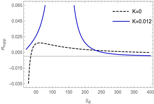
The Ruppeiner scalar versus Kaniadakis entropy plot in the fixed |$(J)$| ensemble for |$l=1$| and |$J=1$|.
4.2. GTD formalism
To describe the rotating BTZ black hole in GTD formalism, we first assume a 5D phase space |$\mathcal {T}$| with coordinates |$M, S, J, T$|, and |$\Omega$|, which are the mass, entropy, angular momentum, temperature, and angular velocity for the black hole. The contact 1-form for this set of coordinates can be written as:
The 1-form satisfies the condition |$\Theta \wedge (d\Theta )^3 \ne 0$| and a Legendre invariant metric that goes by:
We then assume a 2D subspace of |$\mathcal {T}$| with coordinates |$E^a$| where |$a=1,2$|. We denote this subspace by |$\epsilon$|, which is defined as a smooth mapping, |$\phi : \epsilon \rightarrow \mathcal {T}$|. The subspace |$\epsilon$| becomes the space of equilibrium states if the pullback of |$\phi$| is 0, i.e. |$\phi ^{*}(\Theta )=0$|. A metric structure |$g$| is then naturally induced on |$\epsilon$| by applying the same pullback on the metric G of |$\mathcal {T}$|. This induced metric determines all the geometric properties of the equilibrium space for the R-BTZ black hole.
4.2.1. The Kaniadakis entropy case
Fixed |$(J)$| ensemble:
We write the GTD metric for the Kaniadakis entropy case in the fixed |$(J)$| ensemble from the general metric given in Eq. (9). We consider the thermodynamic potential |$\varphi$| to be the mass |$M_K$| for the Kaniadakis entropy case in the fixed |$(J)$| ensemble as obtained in Eq. (15). The GTD metric is given by:
From the above metric we calculate the GTD scalar for the Kaniadakis entropy case in the fixed |$(J)$| ensemble. We have not presented here either the derivation or the final expressions for the GTD scalar due to their considerable length. However, obtaining these expressions is fairly straightforward and involves only routine mathematical computations. We present a detailed analysis of the GTD thermodynamic geometry for the Kaniadakis entropy case in the fixed |$(J)$| ensemble as follows.
We see from Fig. 10 that the GTD scalar |$R_\mathrm{GTD}$| is plotted against the Kaniadakis entropy |$S_K$| for the Kaniadakis parameter |$K=0.012$| in the fixed |$(J)$| ensemble. We find that, for |$l=1$| and |$J=1$|, the GTD scalar has a curvature singularity at |$S_K = 125.77$| for |$K=0.012$| as depicted by the blue solid curve, whereas for the BH entropy case (|$K=0$|) the curve remains regular everywhere with no curvature singularities, as is depicted in the figure by the black dashed curve. Unlike the Ruppeiner scalar, the singularity obtained from the GTD scalar curve exactly matches the point of divergence obtained from the corresponding heat capacity curve for the Kaniadakis entropy case in the fixed |$(J)$| ensemble.
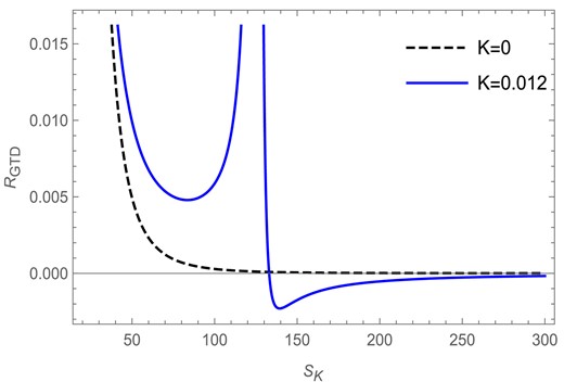
The GTD scalar versus Kaniadakis entropy plot in the fixed |$(J)$| ensemble for |$l=1$| and |$J=1$|.
Fixed |$(\Omega )$| ensemble:
We write the GTD metric for the Kaniadakis entropy case in the fixed |$(\Omega )$| ensemble from the general metric given in Eq. (9). We consider the thermodynamic potential |$\varphi$| to be the mass |$M_K$| for the Kaniadakis entropy case in the fixed |$(\Omega )$| ensemble as obtained in Eq. (21). The GTD metric is given by:
From the above metric we calculate the GTD scalar for the Kaniadakis entropy case in the fixed |$(\Omega )$| ensemble. We have not shown here either the derivation or the final expressions for the GTD scalar due to their considerable length. However, obtaining them is fairly straightforward and involves only routine mathematical computations. We present a detailed analysis of the GTD thermodynamic geometry for the Kaniadakis entropy case in the fixed |$(\Omega )$| ensemble as follows.
We see from Fig. 11 that the GTD scalar |$R_\mathrm{GTD}$| is plotted against the Kaniadakis entropy |$S_{K}$| in the fixed |$(\Omega )$| ensemble. We find that, for |$l=1$| and |$\Omega =0.2$|, the GTD scalar has a curvature singularity at |$S_K =125.74$| for |$K=0.012$| as depicted by the blue solid curve, whereas for the BH entropy case (|$K=0$|) the curve remains regular everywhere with no curvature singularities, as is depicted in the figure by the black dashed curve. Unlike the Ruppeiner scalar, the singularity obtained from the GTD scalar curve exactly matches the point of divergence obtained from the corresponding heat capacity curve for the Kaniadakis entropy case in the fixed |$(\Omega )$| ensemble.
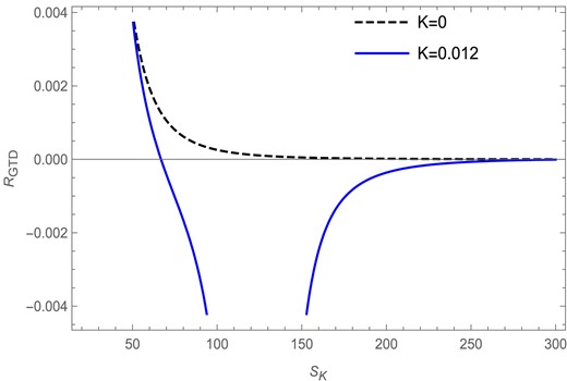
The GTD scalar versus Kaniadakis entropy plot in the fixed |$(\Omega )$| ensemble for |$l=1$| and |$\Omega =0.2$|.
5. Thermodynamics of the charged BTZ black hole
The action that facilitates the field equations [64–66,69,70] from which the |$(2+1)$|D charged BTZ black hole solutions are obtained is given as:
where the AdS length |$l$| is related to the cosmological constant |$\Lambda$| by the relation |$\Lambda =- \frac{1}{l^2}$| and Einstein’s field equations are given by:
the energy–momentum tensor for the same is given as:
The line element that corresponds to the given solution is:
where |$f(r) = -M + \frac{r^2}{l^2} - \frac{\pi Q^2}{2} \ln \left[r\right]$| and M and Q are the mass and electric charge carried by the black hole. Solving the function for |$f(r)=0$| would give us the roots that determine the horizon radius. For an exterior horizon radius |$r_{+}$|, the black hole mass is given by:
and the black hole entropy is given by:
5.1. The Kaniadakis entropy case
Fixed |$(Q)$| ensemble:
We replace the horizon radius in Eq. (34) by the one obtained in Eq. (14) to get the modified mass |$M_{K}$| for the charged BTZ black hole, given by:
The function |$\mathrm{\mathrm{arcsinh}}[K S_{K}]$| can be replaced by its logarithmic form |$\ln [KS_{K}+ \sqrt{1 + K^2 S_{K} ^2}]$| and therefore the expression for mass becomes:
The heat capacity for the Kaniadakis entropy case in the fixed |$(Q)$| ensemble can be obtained as:
where
and
In Fig. 12 the heat capacity |$C_K$| is plotted against the Kaniadakis entropy |$S_K$| for |$l=1$| and |$Q=1$| in the fixed |$(Q)$| ensemble. Here the solid blue curve represents the heat capacity for the Kaniadakis parameter |$K=0.012$|, whereas the black dashed line represents the heat capacity for the BH entropy case |$(K=0)$|. We find that, for |$K=0.012$|, the heat capacity has a divergence at |$S_K=128.82$|, which indicates the presence of a Davies-type phase transition in the Kaniadakis modified black hole, whereas the heat capacity for the BH entropy case shows no such behavior.
The Gibbs free energy for the Kaniadakis entropy case in the fixed |$(Q)$| ensemble can be obtained as:
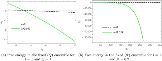
In Figs. 13(a) and (b) the Gibbs free energy |$G_K$| is plotted against the Kaniadakis entropy |$S_K$| for |$l=1$| and |$Q=1$| in the fixed |$(Q)$| ensemble. We draw two different plots so as to make the presence of the phase transitions more transparent. Here the solid blue curve represents the Gibbs free energy for the Kaniadakis parameter |$K=0.012$|, whereas the black dashed line represents the free energy for the BH entropy case |$(K=0)$|. The free energy for the |$K=0$| case has been scaled down by multiplying it by |$\frac{1}{10}$|, whereas the free energy for the |$K=0.012$| case is kept the same; this difference in scaling is just so that the distinct behavior of both the curves can be seen more clearly. We keep in mind that the scaling does not affect the position or occurrence of the phase transitions. We find that in Fig. 13(a) the Gibbs free energy goes to zero for both the entropy cases, where, for |$K=0$|, the zero point is at |$S_K =14.55$| and, for |$K=0.012$|, the zero point is found to be at |$S_K =14.67$|; these zero points refer to the presence of a Hawking–Page phase transition in the rotating BTZ black hole for both the BH as well as the Kaniadakis entropy cases. We again find that, for |$K=0.012$|, the Gibbs free energy in Fig. 13(b) has a zero point at |$S_K=289.97$| only for the Kaniadakis entropy case, which indicates the presence of a Hawking–Page phase transition in the Kaniadakis modified black hole, whereas the Gibbs free energy for the BH entropy case shows no such behavior. In Fig. 13(c) we plot the inverse of specific heat capacity (purple) and the Gibbs free energy (orange) against the Kaniadakis entropy. The inverse of specific heat capacity has been scaled up by multiplying it by 3000, whereas the free energy is kept the same; this difference in scaling is just so that the distinct behavior of both the curves can be seen more clearly. We keep in mind that the scaling does not affect the position or occurrence of the phase transitions. The points where these curves intersect the horizontal axis represent the Davies-type (purple) and Hawking–Page (orange) phase transitions respectively, which are seen to be quite distant from each other.
The heat capacity versus Kaniadakis entropy plot in the fixed |$(Q)$| ensemble for |$l=1$| and |$Q=1$|.
The Gibbs free energy curves for Kaniadakis entropy in the fixed |$(Q)$| ensemble for |$l=1$| and |$Q=1$|.
Fixed |$(\Phi )$| ensemble:
The modified mass for the Kaniadakis entropy case in the fixed |$(\Phi )$| ensemble is given by:
where |$\frac{\partial M_{K}}{\partial Q}= \Phi$| is the electric potential of the black hole with respect to the electric charge |$Q$|. By writing the term |$M_{K} ^{\prime }$| as |$M_{K}$| for convenience we get:
The heat capacity for the Kaniadakis entropy case in the fixed |$(\Phi )$| ensemble can be obtained as:
where
and
In Fig. 14 the heat capacity |$C_K$| for the charged BTZ black hole is plotted against the Kaniadakis entropy |$S_K$| in the fixed |$(\Phi )$| ensemble. We draw the same plot in two different entropy ranges so as to make all the divergences appearing in the heat capacity curve visible. We see from Fig. 14(a) that for |$l=1$| and |$\Phi =0.2$| there is a divergence at |$S_K=10.26$| for |$K=0.012$| as shown by the solid blue curve. The heat capacity in the BH entropy case (|$K=0)$| here also produces a divergence at |$S_K=10.24$| as shown by the black dashed curve. In Fig. 14(b) we see that there is a divergence in the heat capacity curve at |$S_K=125.74$| for |$K=0.012$|, whereas here the heat capacity in the BH entropy case |$(K=0)$| remains a monotonically increasing function of entropy with no divergences.
The heat capacity versus Kaniadakis entropy plot in the fixed |$(\Phi )$| ensemble for |$l=1$| and |$\Phi =0.2$|.
The Gibbs free energy for the Kaniadakis entropy case in the fixed |$(\Phi )$| ensemble can be obtained as:
where
and
In Fig. 15(a) the Gibbs free energy |$G_K$| is plotted against the Kaniadakis entropy |$S_K$| for |$l=1$| and |$\Phi =0.2$| in the fixed |$(\Phi )$| ensemble. Here the solid blue curve represents the Gibbs free energy for the Kaniadakis parameter |$K=0.012$|, whereas the black dashed line represents the free energy for the BH entropy case |$(K=0)$|. The free energy for the |$K=0$| case has been scaled down by multiplying it by |$\frac{1}{10}$|, whereas the free energy for the |$K=0.012$| case is kept the same; this difference in scaling is just so that the distinct behavior of both the curves can be seen more clearly. We keep in mind that the scaling does not affect the position or occurrence of the phase transition. We find that, for |$K=0.012$|, the Gibbs free energy has a zero point at |$S_K=276.64$|, which indicates the presence of a Hawking–Page phase transition in the Kaniadakis modified black hole, whereas the Gibbs free energy for the BH entropy case shows no such behavior. In Fig. 15(b) we plot the inverse of specific heat capacity (purple) and the Gibbs free energy (orange) against the Kaniadakis entropy. The inverse of specific heat capacity has been scaled up by multiplying it by 3000, whereas the free energy is kept the same; this difference in scaling is just so that the distinct behavior of both the curves can be seen more clearly. We keep in mind that the scaling does not affect the position or occurrence of the phase transitions. The points where these curves intersect the horizontal axis represent the Davies-type (purple) and Hawking–Page (orange) phase transitions respectively, which are seen to be quite distant from each other.
The Gibbs free energy curves for Kaniadakis entropy in the fixed |$(\Phi )$| ensemble for |$l=1$| and |$\Phi =0.2$|.
5.2. The Renyi entropy case
Fixed |$(Q)$| ensemble:
We replace the horizon radius in Eq. (34) by the one obtained in Eq. (23) to get the modified mass |$M_{R}$| for the charged BTZ black hole, given by:
The heat capacity for the Renyi entropy case in the fixed |$(Q)$| ensemble can be calculated as:
We see from Fig. 16(a) that the heat capacity |$C_R$| for the charged BTZ black hole is plotted against the Renyi entropy |$S_R$| in the fixed |$(Q)$| ensemble. Here the solid green curve represents the heat capacity for the Renyi parameter |$\lambda =0.012$|, whereas the black dashed line represents the heat capacity for the BH entropy case |$(\lambda =0)$|. For the parameters |$l=1$| and |$ Q=1$| we find that there are no divergences in the heat capacity curve for both the Renyi and BH entropy cases.
The heat capacity versus Renyi entropy plots in the fixed |$(J)$| and fixed |$(\Phi )$| ensembles.
The Gibbs free energy for the Renyi entropy case in the fixed |$(Q)$| ensemble can be obtained as:
In Fig. 17(a) the Gibbs free energy |$G_R$| is plotted against the Renyi entropy |$S_R$| for |$l=1$| and |$Q=1$| in the fixed |$(Q)$| ensemble. Here the solid green curve represents the Gibbs free energy for the Renyi parameter |$\lambda =0.012$|, whereas the black dashed line represents the free energy for the BH entropy case |$(\lambda =0)$|. The free energy for the |$\lambda =0$| case has been scaled down by multiplying it by |$\frac{1}{10}$|, whereas the free energy for the |$\lambda =0.012$| case is kept the same; this difference in scaling is just so that the distinct behavior of both the curves can be seen more clearly. We find that in Fig. 17(a) the Gibbs free energy goes to zero for both the entropy cases, where, for |$\lambda =0$|, the zero point is at |$S_R =14.55$| and, for |$\lambda =0.012$|, the zero point is found to be at |$S_R =13.17$|; these zero points refer to the presence of a Hawking–Page phase transition in the charged BTZ black hole for both the BH as well as the Renyi entropy cases.
The Gibbs free energy versus Renyi entropy plots in the fixed |$(Q)$| and fixed |$(\Phi )$| ensembles.
Fixed |$(\Phi )$| ensemble:
The modified mass for the Renyi entropy case in the fixed |$(\Phi )$| ensemble is given by:
where |$\frac{\partial M_{R}}{\partial Q}= \Phi$| is the electric potential of the black hole with respect to the electric charge |$Q$|. By making the necessary replacements and putting |$l=1$|, we get the final equation as follows:
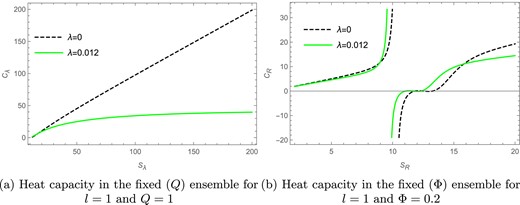
We have here used the term |$M_{R}$| instead of |$M_{R}^{\prime }$| for convenience. Here |$M_{R}$| is the modified mass for the fixed |$(\Phi )$| ensemble. The heat capacity for the Renyi entropy case in the fixed |$(\Phi )$| ensemble can be calculated as:
where
We see from Fig. 16(b) that the heat capacity |$C_R$| for the charged BTZ black hole is plotted against the Renyi entropy |$S_R$| in the fixed |$(\Phi )$| ensemble. Here the solid green curve represents the heat capacity for the Renyi parameter |$\lambda =0.012$|, whereas the black dashed line represents the heat capacity for the BH entropy case |$(\lambda =0)$|. We see that for |$l=1$| and |$\Phi =0.2$| there is a divergence in the heat capacity curve for both the Renyi and BH entropy cases. The divergence for the Renyi entropy case |$(K=0.012)$| is seen to be at |$S_{K}=9.71$|, whereas for the BH entropy case |$(K=0)$| the divergence is found to be at |$S_{K}=10.24$|.
The Gibbs free energy for the Renyi entropy case in the fixed |$(\Phi )$| ensemble can be obtained as:
where
In Fig. 17(b) the Gibbs free energy |$G_R$| is plotted against the Renyi entropy |$S_R$| for |$l=1$| and |$\Phi =0.2$| in the fixed |$(\Phi )$| ensemble. Here the solid green curve represents the Gibbs free energy for the Renyi parameter |$\lambda =0.012$|, whereas the black dashed line represents the free energy for the BH entropy case |$(\lambda =0)$|. The free energy for the |$\lambda =0$| case has been scaled down by multiplying it by |$\frac{1}{10}$|, whereas the free energy for the |$\lambda =0.012$| case is kept the same; this difference in scaling is just so that the distinct behavior of both the curves can be seen more clearly. We find that, unlike the Kaniadakis entropy, there is no Hawking–Page phase transition present in the Renyi entropy case for the fixed |$(\Phi )$| ensemble.
5.3. The Barrow entropy case
Fixed |$(Q)$| ensemble:
We replace the horizon radius in Eq. (34) by the one obtained in Eq. (30) to get the modified mass |$M_{\Delta }$| for the charged BTZ black hole, given by:
The heat capacity for the Barrow entropy case in the fixed |$(Q)$| ensemble can be calculated as:
We see from Fig. 18(a) that the heat capacity |$C_{\Delta }$| for the charged BTZ black hole is plotted against the Barrow entropy |$S_{\Delta }$| in the fixed |$(Q)$| ensemble. Here the solid red curve represents the heat capacity for the Barrow parameter |$\Delta =0.012$|, whereas the black dashed line represents the heat capacity for the BH entropy case |$(\Delta =0)$|. For the parameters |$l=1$| and |$ Q=1$| we find that there are no divergences in the heat capacity curve for both the Barrow and BH entropy cases.
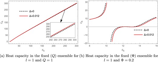
The heat capacity versus Barrow entropy plots in the fixed |$(J)$| and fixed |$(\Phi )$| ensembles.
The Gibbs free energy for the Renyi entropy case in the fixed |$(Q)$| ensemble can be obtained as:
In Fig. 19(a) the Gibbs free energy |$G_\Delta$| is plotted against the Barrow entropy |$S_\Delta$| for |$l=1$| and |$Q=1$| in the fixed |$(Q)$| ensemble. Here the solid red curve represents the Gibbs free energy for the Barrow parameter |$\Delta =0.012$|, whereas the black dashed line represents the free energy for the BH entropy case |$(\Delta =0)$|. The free energy for the |$\Delta =0$| case has been scaled down by multiplying it by |$\frac{1}{10}$|, whereas the free energy for the |$\Delta =0.012$| case is kept the same; this difference in scaling is just so that the distinct behavior of both the curves can be seen more clearly. We find that in Fig. 19(a) the Gibbs free energy goes to zero for both the entropy cases, where, for |$\Delta =0$|, the zero point is at |$S_\Delta =14.55$| and, for |$\Delta =0.012$|, the zero point is found to be at |$S_\Delta =14.81$|; these zero points refer to the presence of a Hawking–Page phase transition in the charged BTZ black hole for both the BH as well as the Barrow entropy cases.
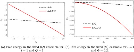
The Gibbs free energy versus Barrow entropy plots in the fixed |$(Q)$| and fixed |$(\Phi )$| ensembles.
Fixed |$(\Phi )$| ensemble:
The modified mass for the Barrow entropy case in the fixed |$(\Phi )$| ensemble is given by:
where |$\frac{\partial M_{\Delta }}{\partial Q}= \Phi$| is the electric potential of the black hole with respect to the electric charge |$Q$|. By making the necessary replacements and putting |$l=1$|, we get the final equation as follows:
We have here used the term |$M_{\Delta }$| instead of |$M_{\Delta }^{\prime }$| for convenience. Here |$M_{\Delta }$| is the modified mass for the fixed |$(\Phi )$| ensemble. The heat capacity for the Barrow entropy case in the fixed |$(\Phi )$| ensemble can be calculated as:
where
and
We see from Fig. 18(b) that the heat capacity |$C_{\Delta }$| for the charged BTZ black hole is plotted against the Barrow entropy |$S_{\Delta }$| in the fixed |$(\Phi )$| ensemble. Here the solid red curve represents the heat capacity for the Barrow parameter |$\Delta =0.012$|, whereas the black dashed line represents the free energy for the BH entropy case |$(\Delta =0)$|. We see that for |$l=1$| and |$\Phi =0.2$| there is a divergence in the heat capacity curve for both the Barrow and BH entropy cases. The divergence for the Barrow entropy case |$(\Delta =0.012)$| is seen to be at |$S_{\Delta }=10.37$|, whereas for the BH entropy case |$(\Delta =0)$| the divergence is found to be at |$S_{\Delta }=10.24$|.
The Gibbs free energy for the Barrow entropy case in the fixed |$(\Phi )$| ensemble can be obtained as:
In Fig. 19(b) the Gibbs free energy |$G_\Delta$| is plotted against the Barrow entropy |$S_\Delta$| for |$l=1$| and |$\Phi =0.2$| in the fixed |$(\Phi )$| ensemble. Here the solid red curve represents the Gibbs free energy for the Barrow parameter |$\Delta =0.012$|, whereas the black dashed line represents the free energy for the BH entropy case |$(\Delta =0)$|. The free energy for the |$\Delta =0$| case has been scaled down by multiplying it by |$\frac{1}{10}$|, whereas the free energy for the |$\Delta =0.012$| case is kept the same; this difference in scaling is just so that the distinct behavior of both the curves can be seen more clearly. We find that, unlike the Kaniadakis entropy, there is no Hawking–Page phase transition present in the Barrow entropy case for the fixed |$(\Phi )$| ensemble.
6. Thermodynamic geometry of the charged BTZ black hole
We discuss the thermodynamic geometry of the charged BTZ black hole for both the Ruppeiner and GTD formalisms. The Ruppeiner metric is defined as the negative Hessian of entropy with respect to other extensive variables. Therefore it is only the fixed |$(Q)$| ensemble, which holds good in the Ruppeiner formalism as |$Q$| is an extensive thermodynamic quantity, whereas |$\Phi$| is not.
Therefore the fixed |$(\Phi )$| ensemble does not hold good as per the definition of the Ruppeiner metric. We therefore discuss the thermodynamic geometry of the fixed |$(\Phi )$| ensemble in the GTD formalism, which is defined on a multidimensional phase space that comprises both the extensive and intensive variables of the thermodynamic system. The GTD formalism is therefore the appropriate geometric formalism for discussing both the thermodynamic ensembles.
We first discuss the Ruppeiner geometry of the charged BTZ black hole in the fixed |$(Q)$| ensemble where we observe a curvature singularity in the Ruppeiner scalar curve only for the Kaniadakis entropy case. We then discuss the GTD geometry of the black hole for both the thermodynamic ensembles, where we observe curvature singularities in the GTD scalar curves in the Kaniadakis entropy case only. These curvature singularities are seen to occur exactly at the points where we saw divergences in the corresponding heat capacity curves in the previous section.
6.1. Ruppeiner formalism
The Ruppeiner metric for the C-BTZ black hole in the fixed |$(Q)$| ensemble can be obtained from the relation (8) and is given as:
where |$M$|, |$S$|, |$T$|, and |$Q$| are the mass, entropy, Hawking temperature, and electric charge for the charged BTZ black hole respectively.
From the above metric we calculate the Ruppeiner scalar for all the nonextensive entropy cases in the fixed |$(Q)$| ensemble. We find that there is a curvature singularity in the Ruppeiner scalar curve only for the Kaniadakis entropy case. For all the other entropy cases, namely the Renyi and Barrow entropy cases, the Ruppeiner scalar curves remain regular with no singularities therein. We have not presented here either the derivation or the final expressions for the Ruppeiner scalar due to their considerable length. However, obtaining these expressions is fairly straightforward and involves only routine mathematical computations. We present a detailed analysis of the Ruppeiner thermodynamic geometry for the Kaniadakis entropy case in the fixed |$(Q)$| ensemble as follows.
We see from Fig. 20 that the Ruppeiner scalar |$R_\mathrm{Rupp}$| is plotted against the Kaniadakis entropy |$S_K$| in the fixed |$(Q)$| ensemble. We see that, for |$l=1$| and |$Q=1$|, for the Kaniadakis parameter |$K=0.012$| the Ruppeiner scalar curve has a curvature singularity specifically at |$S_K = 128.82$|, which is depicted by the solid blue curve in the figure. The point of singularity here, unlike for the rotating BTZ black hole, is similar to the point of divergence obtained in the corresponding heat capacity curve for the Kaniadakis entropy case in the fixed |$(Q)$| ensemble. For the |$K=0$| case, however, the Ruppeiner scalar curve is found to be regular everywhere with no curvature singularities, as is depicted in the figure by the black dashed curve.
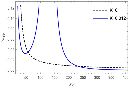
The Ruppeiner scalar versus Kaniadakis entropy plot in the fixed |$(Q)$| ensemble for |$l=1$| and |$Q=1$|.
6.2. GTD formalism
To describe the charged BTZ black hole in GTD formalism, we first assume a 5D phase space |$\mathcal {T}$| with coordinates |$M, S, Q, T$|, and |$\Phi$|, which are the mass, entropy, electric charge, temperature, and electric potential for the black hole. The contact 1-form for this set of coordinates can be written as:
The 1-form satisfies the condition |$\Theta \wedge (d\Theta )^3 \ne 0$| and a Legendre invariant metric that goes by:
We then assume a 2D subspace of |$\mathcal {T}$| with coordinates |$E^a$| where |$a=1,2$|. We denote this subspace by |$\epsilon$|, which is defined as a smooth mapping, |$\phi : \epsilon \rightarrow \mathcal {T}$|. The subspace |$\epsilon$| becomes the space of equilibrium states if the pullback of |$\phi$| is 0, i.e. |$\phi ^{*}(\Theta )=0$|. A metric structure |$g$| is then naturally induced on |$\epsilon$| by applying the same pullback on the metric G of |$\mathcal {T}$|. This induced metric determines all the geometric properties of the equilibrium space for the charged BTZ black hole.
6.2.1. The Kaniadakis entropy case
Fixed |$(Q)$| ensemble:
We write the GTD metric for the Kaniadakis entropy case in the fixed |$(Q)$| ensemble from the general metric given in Eq. (9). We consider the thermodynamic potential |$\varphi$| to be the mass |$M_K$| for the Kaniadakis entropy case in the fixed |$(Q)$| ensemble as obtained in Eq. (15). The GTD metric is given by:
From the above metric we calculate the GTD scalar for the Kaniadakis entropy case in the fixed |$(Q)$| ensemble. We have not presented here either the derivation or the final expressions for the GTD scalar due to their considerable length. However, obtaining these expressions is fairly straightforward and involves only routine mathematical computations. We present a detailed analysis of the GTD thermodynamic geometry for the Kaniadakis entropy case in the fixed |$(Q)$| ensemble as follows.
We see from Fig. 21 that the GTD scalar |$R_\mathrm{GTD}$| is plotted against the Kaniadakis entropy |$S_K$| for the Kaniadakis parameter |$K=0.012$| in the fixed |$(Q)$| ensemble. We find that, for |$l=1$| and |$Q=1$|, the GTD scalar has a curvature singularity at |$S_K = 128.82$| for |$K=0.012$| as depicted by the blue solid curve, whereas for the BH entropy case (|$K=0$|) the curve remains regular everywhere with no curvature singularities, as is depicted in the figure by the black dashed curve. The singularity obtained from the GTD scalar curve exactly matches the point of divergence obtained from the corresponding heat capacity curve for the Kaniadakis entropy case in the fixed |$(Q)$| ensemble.
The GTD scalar versus Kaniadakis entropy plot in the fixed |$(Q)$| ensemble for |$l=1$| and |$Q=1$|.
Fixed |$(\Phi )$| ensemble:
We write the GTD metric for the Kaniadakis entropy case in the fixed |$(\Phi )$| ensemble from the general metric given in Eq. (9). We consider the thermodynamic potential |$\varphi$| to be the mass |$M_K$| for the Kaniadakis entropy case in the fixed |$(\Phi )$| ensemble as obtained in Eq. (21). The GTD metric is given by:
From the above metric we calculate the GTD scalar for the Kaniadakis entropy case in the fixed |$(\Phi )$| ensemble. We have not shown here either the derivation or the final expressions for the GTD scalar due to their considerable length. However, obtaining them is fairly straightforward and involves only routine mathematical computations. We present a detailed analysis of the GTD thermodynamic geometry for the Kaniadakis entropy case in the fixed |$(\Phi )$| ensemble as follows.
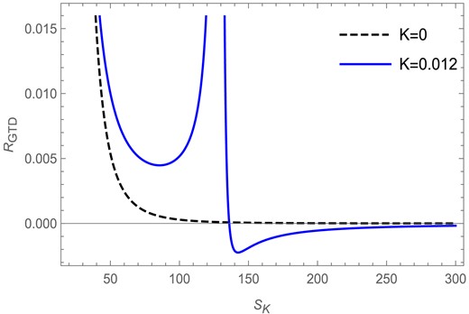
In Fig. 22 the GTD scalar |$R_\mathrm{GTD}$| for the charged BTZ black hole is plotted against the Kaniadakis entropy |$S_K$| in the fixed |$(\Phi )$| ensemble. We draw the same plot in two different entropy ranges so as to make all the singularities appearing in the GTD scalar curve visible. We see from Fig. 22(a) that for |$l=1$| and |$\Phi =0.2$| there is a singularity at |$S_K=10.26$| for |$K=0.012$| as shown by the solid blue curve. The heat capacity in the BH entropy case (|$K=0)$| here also produces a singularity at |$S_K=10.24$| as shown by the black dashed curve. Although we can see the presence of two additional curvature singularities observed in the figure for both the Kaniadakis and BH entropy cases, it was found that these additional curvature singularities correspond to the points where the heat capacity goes to zero for both the Kaniadakis and BH entropy cases in the fixed |$(\Phi )$| ensemble. In Fig. 22(b) we see that there is a singularity in the heat capacity curve at |$S_K=125.74$| for |$K=0.012$|, whereas here for the |$(K=0)$| case no such behavior is observed in the GTD scalar curve.
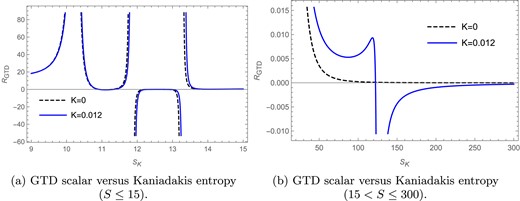
The GTD scalar versus Kaniadakis entropy plot in the fixed |$(\Omega )$| ensemble for |$l=1$| and |$\Phi =0.2$|.
6.2.2. The Renyi entropy case
Fixed |$(\Phi )$| ensemble:
We write the GTD metric for the Renyi entropy case in the fixed |$(\Phi )$| ensemble from the general metric given in Eq. (9). We consider the thermodynamic potential |$\varphi$| to be the mass |$M_K$| for the Renyi entropy case in the fixed |$(\Phi )$| ensemble. The GTD metric is given by:
From the above metric we calculate the GTD scalar for the Renyi entropy case in the fixed |$(\Phi )$| ensemble. We have not shown here either the derivation or the final expressions for the GTD scalar due to their considerable length. However, obtaining them is fairly straightforward and involves only routine mathematical computations. We present a detailed analysis of the GTD thermodynamic geometry for the Renyi entropy case in the fixed |$(\Phi )$| ensemble as follows.
We see from Fig. 23 that the GTD scalar |$R_\mathrm{GTD}$| for the charged BTZ black hole is plotted against the Renyi entropy |$S_R$| in the fixed |$(\Phi )$| ensemble. We see that for |$l=1$| and |$\Phi =0.2$| there are curvature singularities in the GTD scalar curve for both the Renyi |$(\lambda =0.012)$| and BH entropy |$(\lambda =0)$| cases. We find that, for |$\lambda =0.012$|, there is a curvature singularity observed in the GTD scalar curve at |$S_R=9.71$| as depicted by the solid green curve in the figure. For the BH entropy case (|$\lambda =0$|) we find that the GTD scalar has a curvature singularity at |$S_R=10.24$| as shown in the figure by the black dashed curve. These singularities exactly match the points of Davies-type phase transitions observed in the corresponding heat capacity curve in the fixed |$(\Phi )$| ensemble. There are two additional curvature singularities observed in the figure for both the Renyi and BH entropy cases; however, it was found that these additional curvature singularities correspond to the points where the heat capacity goes to zero for both the Renyi and BH entropy cases in the fixed |$(\Phi )$| ensemble.
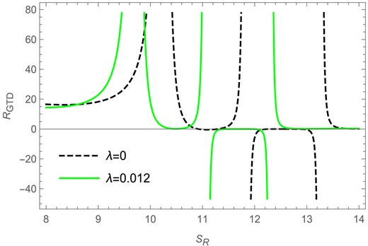
The GTD scalar versus Renyi entropy plot in the fixed |$(\Phi )$| ensemble for |$l=1$| and |$\Phi =0.2$|.
6.2.3. The Barrow entropy case
Fixed |$(\Phi )$| ensemble:
We write the GTD metric for the Barrow entropy case in the fixed |$(\Phi )$| ensemble from the general metric given in Eq. (9). We consider the thermodynamic potential |$\varphi$| to be the mass |$M_{\Delta }$| for the Barrow entropy case in the fixed |$(\Phi )$| ensemble. The GTD metric is given by:
From the above metric we calculate the GTD scalar for the Barrow entropy case in the fixed |$(\Phi )$| ensemble. We have not shown here either the derivation or the final expressions for the GTD scalar due to their considerable length. However, obtaining them is fairly straightforward and involves only routine mathematical computations. We present a detailed analysis of the GTD thermodynamic geometry for the Barrow entropy case in the fixed |$(\Phi )$| ensemble as follows.
We see from Fig. 24 that the GTD scalar |$R_\mathrm{GTD}$| for the charged BTZ black hole is plotted against the Barrow entropy |$S_{\Delta }$| in the fixed |$(\Phi )$| ensemble. We see that for |$l=1$| and |$\Phi =0.2$| there are curvature singularities in the GTD scalar curve for both the Barrow |$(\Delta =0.012)$| and BH entropy |$(\Delta =0)$| cases. We find that, for |$\Delta =0.012$|, there is a curvature singularity observed in the GTD scalar curve at |$S_{\Delta }=10.37$| as depicted by the solid red curve in the figure. For the BH entropy case (|$\Delta =0$|) we find that the GTD scalar has a curvature singularity at |$S_{\Delta }=10.24$| as shown in the figure by the black dashed curve. These singularities exactly match the points of Davies-type phase transitions observed in the corresponding heat capacity curve in the fixed |$(\Phi )$| ensemble. There are two additional curvature singularities observed in the figure for both the Barrow and BH entropy cases; however, it was found that these additional curvature singularities correspond to the points where the heat capacity goes to zero for both the Barrow and BH entropy cases in the fixed |$(\Phi )$| ensemble.
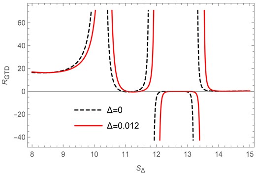
The GTD scalar versus Barrow entropy plot in the fixed |$(\Phi )$| ensemble for |$l=1$| and |$\Phi =0.2$|.
7. Conclusions
We investigated the thermodynamics and thermodynamic geometry of rotating (R-BTZ) and charged (C-BTZ) Banados–Teitelboim–Zanelli black holes in three different nonextensive entropy formalisms, namely the Kaniadakis entropy, Renyi entropy, and Barrow entropy respectively. We investigated all the thermodynamic ensembles of these black holes, namely the fixed |$(J)$| and fixed |$(\Omega )$| ensembles for the rotating BTZ black hole and the fixed |$(Q)$| and fixed |$(\Phi )$| ensembles for the charged BTZ black hole. We find that there are Davies-type and Hawking–Page phase transitions in both the black holes observed in the Kaniadakis entropy case for all the thermodynamic ensembles. We found that both the Ruppeiner and the GTD scalar were observed to have curvature singularities corresponding to Davies-type phase transitions in the corresponding cases. The location of the curvature singularities in the GTD scalar exactly matched the Davies-type phase transition points in both the ensembles. Although the Ruppeiner scalar showed curvature singularities, the locations of those singularities were found to be not exactly the same as the corresponding Davies-type transition points for the R-BTZ black hole. For all the other nonextensive entropy cases, the thermodynamic structures were found to resemble their counterparts in the BH entropy. Tables 1 and 2summarize our results, in which we give the number of phase transition points (both Davies-type and Hawking–Page) observed against each of the nonextensive entropy cases along with the BH entropy for all the thermodynamic ensembles.
Results for the R-BTZ black hole.
| Entropy | Fixed (J) ensemble | Fixed (|$\Omega$|) ensemble | ||
|---|---|---|---|---|
| Davies-type | Hawking–Page | Davies-type | Hawking–Page | |
| phase transition | phase transition | phase transition | phase transition | |
| BH | 0 | 1 | 0 | 0 |
| Kaniadakis | 1 | 2 | 1 | 1 |
| Renyi | 0 | 1 | 0 | 0 |
| Barrow | 0 | 1 | 0 | 0 |
Results for the C-BTZ black hole.
| Entropy | Fixed (Q) ensemble | Fixed (|$\Phi$|) ensemble | ||
|---|---|---|---|---|
| Davies-type | Hawking–Page | Davies-type | Hawking–Page | |
| phase transition | phase transition | phase transition | phase transition | |
| BH | 0 | 1 | 1 | 0 |
| Kaniadakis | 1 | 2 | 2 | 1 |
| Renyi | 0 | 1 | 1 | 0 |
| Barrow | 0 | 1 | 1 | 0 |
The key distinction of Kaniadakis entropy lies in its impact on the behavior of black hole temperature. In contrast to the other considered entropic formalisms, where temperature is a monotonically increasing function of entropy, Kaniadakis entropy introduces a different thermal evolution. We have observed that, in the Kaniadakis entropy framework, black hole temperature rises to a maximum value before gradually declining and asymptotically tending to zero for larger values of entropy. This nonmonotonic behavior in the temperature is what gives rise to the advent of the phase transitions (both Davies-type and Hawking–Page) in the specific heat capacity and the Gibbs free energy respectively for the rotating and charged BTZ black holes. The behavior of temperature in the R-BTZ black hole for both the Kaniadakis and BH entropy cases is depicted in Fig. 25.
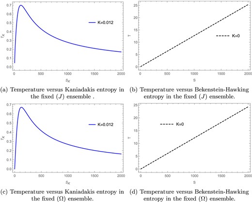
The temperature curves for Kaniadakis entropy in the fixed |$(J)$| and |$(\Omega )$| ensembles for |$l=1,J=1$|, and |$\Omega =0.2$|.
We know that the specific heat capacity of a black hole is given by |$C=\frac{T}{(\frac{\partial T}{\partial S})}$|. Thus, when the temperature attains its maximum value, the slope of the graph, i.e. |$\frac{\partial T}{\partial S}$|, equals zero and the specific heat capacity undergoes a divergence. When the temperature starts decreasing, the slope of the T–S graph becomes negative and so does the heat capacity. We also know that the black hole temperature is a first-order derivative of mass with respect to entropy, i.e. |$T=(\frac{\partial M}{\partial S})$|, where the mass M for the rotating BTZ black hole is given by:
where writing the BH entropy |$S_\mathrm{BH}$| in terms of the Kaniadakis entropy, i.e. |$S_\mathrm{BH} = \frac{\mathrm{arcsinh}(K S)}{ K}$|, gives the Kaniadakis corrected mass, which is given by:
It is actually the second term in the above equation that is responsible for the unusual behavior in the temperature of the black hole. Here, the term |$ \frac{\mathrm{\mathrm{arcsinh}}^2 [K S]}{16 \pi ^2 l^2 K^2}$|, when differentiated with respect to the entropy in order to obtain the temperature, becomes |$ \frac{\mathrm{\mathrm{arcsinh}} [K S]}{ 8 \pi l K \sqrt{1 + K^2 S^2}}$|. This term is directly responsible for the dipping behavior in the temperature because here, as |$\frac{\mathrm{\mathrm{arcsinh}} [K S]}{K}$| is an increasing function of entropy, the term |$\frac{1}{\sqrt{1 + K^2 S^2}}$| decreases with an increase in entropy, and thus they together produce this unusual behavior in the temperature where it starts to fall after reaching a maximum value. The value of the maximum attainable temperature for a given set of |$(J,l)$| values is fixed by the Kaniadakis parameter K, as is evident from the above analysis. The nontrivial temperature profile in the Kaniadakis entropy formalism is also responsible for the Hawking–Page phase transition obtained from the Gibbs free energy of the black hole. The Gibbs free energy is given by |$G = M - T S$|, where the Gibbs free energy is negative for small entropy values; however, as temperature starts falling after having attained its maximum value, |$G$| starts to increase and finally reaches a zero point. On further increase in entropy the free energy becomes positive and thus the black hole becomes thermodynamically unstable, as can be seen from Figs. 2 and 4. The case is similar for the charged BTZ black hole where the Kaniadakis corrected mass for the C-BTZ black hole is given by:
It can be seen here as well that the term |$ \frac{\mathrm{\mathrm{arcsinh}}^2 [K S]}{16 \pi ^2 l^2 K^2}$|, when differentiated with respect to the entropy in order to obtain the temperature, becomes |$ \frac{\mathrm{\mathrm{arcsinh}} [K S]}{ 8 \pi l K \sqrt{1 + K^2 S^2}}$|. We therefore observe the dip in the temperature here as well, which in turn results in the occurrence of a Davies-type phase transition accompanied by a Hawking–Page phase transition in the charged BTZ black hole.
This unusual behavior of the temperature in the Kaniadakis entropy case seems to be inherent in the formulation of this entropy, where it has been shown in Ref. [49] that its mathematical structure is compatible with Einstein’s special theory of relativity along with the second law of thermodynamics. It was also seen in Ref. [71], where the author showed that the corrections in the black hole entropy obtained by Kaniadakis statistics at the high-temperature limit are indeed logarithmic in nature, which prove that these corrections are indeed legitimate. We could not find any specific reasons why a relativistic statistical approach to black holes should cause the temperature to behave so nontrivially. It would perhaps need a more sophisticated analysis of black holes in the Kaniadakis formalism and also Kaniadakis entropy in general to find out why such nontriviality should occur.
To conclude, our analysis shows that the thermodynamic phase structure of |$(2+1)$|D BTZ black holes with Kaniadakis entropy differs from that with the conventional BH entropy in all the ensembles. This result is in contrast to that found in Ref. [14], in the context of charged AdS black holes where both Kaniadakis entropy and BH entropy yielded similar phase structures. It will be interesting to extend the study of black hole thermodynamics in the framework of nonextensive entropy to other black holes to get a clearer picture. We plan to address this issue in our future work.
Acknowledgments
The authors would like to thank Himanshu Bora for numerous enlightening discussions and certain exquisite suggestions that he offered during the course of this work.
Funding
Open Access funding: SCOAP3.
