


Abstract
We investigate the dynamical generation of the |$D_{s0}^{*}(2317)$| and |$B_{s0}^{*}$| mesons using a meson-exchange model with a coupled-channel formalism. Our primary focus is on the |$D_s^+\pi ^0$| channel below the |$DK$| threshold. First, we construct the invariant kernel amplitudes, incorporating effective Lagrangians based on heavy-quark symmetry, flavor SU(3) symmetry, and hidden local symmetry. Since the |$D_{s0}^{*}(2317)$| state implies isospin symmetry breaking, we introduce |$\pi ^0\!-\!\eta$| isospin mixing. We subsequently solve the coupled-channel integral equations, which include four different channels, i.e. |$D_s^+\pi ^0$|, |$D^0 K^+$|, |$D^+ K^0$|, and |$D_s^+\eta$|. We carefully analyze how the pole corresponding to the |$D_{s0}^{*}(2317)$| state emerges from the coupled channels. Our findings reveal that the pole positions of the |$D_{s0}^{*}(2317)$| meson are at |$\sqrt{s_R}=(2317.9 - i 0.0593)$| MeV and those of the |$\bar{B}_{s0}^{*}$| meson are at |$(5756.43-i0.0215)$| MeV, respectively. We also discuss their decay widths and destructive interference of the two sources. In conclusion, our current results provide a clear indication supporting the interpretation of the |$D_{s0}^{*}(2317)$| meson as a |$DK$| molecular state within the present coupled-channel formalism. In addition, we discuss the possible existence of |$\bar{B}_{s0}^{*}$|.
1. Introduction
The |$D_{s0}^{*}(2317)$| meson was initially discovered in 2003 by the BaBar Collaboration while analyzing the inclusive |$D_s^+\pi ^0$| invariant mass distribution from |$e^+e^-$| annihilation data [1]. It was assigned a spin-parity of |$J^P=0^+$|. Subsequently, both the CLEO and Belle Collaborations confirmed the existence of this state [2,3]. Recently, the BESIII Collaboration made an announcement that rekindled interest in the structure of |$D_{s0}^{*}(2317)$|. They observed it with a statistical significance of |$5.8\sigma$| and determined its mass to be |$(2318.3\pm 1.2 \pm 1.2)$| MeV. Furthermore, they measured, for the first time, the absolute branching ratio of |$D_{s0}^{*}(2317)^{\pm }\rightarrow D_s^\pm \pi ^0$| and found it to be |$1.00_{-0.14}^{+0.00} \mbox{(stat)}{}{-0.14}^{+0.00} \mbox{(syst)}$| [4]. Initially, it was assumed that the |$D_{s0}^{*}(2317)$| meson is a conventional P-wave |$c\bar{s}$| state with |$J^P=0^+$| [5,6]. However, the observed mass based on this assumption turned out to be approximately 150 MeV lower than the results from quark models and lattice calculations [5–11]. This discrepancy led to suggestions that the |$D_{s0}^{*}(2317)$| meson could be a non-|$Q\bar{q}$| state, such as a molecular or tetraquark state [12–26].
|$D_{s0}^{*}(2317)$| lies in the proximity of the |$DK$| threshold, being located about 45 MeV below it. This suggests the possibility of considering it as a |$DK$| molecular state. Furthermore, the decay width of the |$D_{s0}^{*}(2317)$| meson is observed to be extremely narrow, with only an upper limit known: |$\Gamma \lt 3.8$| MeV at the |$95\%$| confidence level [27]. This narrow decay width can be attributed to the strong isospin violation involved in the |$D_{s0}^{*}(2317)\rightarrow D_s\pi$| decay. Several theoretical approaches have been proposed to explain the decay modes of |$D_{s0}^{*}(2317)$| [21,25,26,28–32]. Given that |$D_{s0}^{*}(2317)$| is just below the |$DK$| threshold, it is reasonable to investigate its nature as a dynamically generated |$DK$| molecular state. Several theoretical works have provided strong support for this hypothesis. For instance, in Refs. [16–20,26,33,34], it was shown through the coupled-channel formalism that |$D_{s0}^{*}(2317)$| can indeed be dynamically generated. These works considered the |$D_s\eta$| channel, taking into account the |$\pi ^0\!-\!\eta$| mixing. Lattice calculations have also considered the coupled-channel effects. For example, Mohler et al. [24] considered both the |$c\bar{s}$| and |$DK$| interpolators, while in Refs. [25,31,35–37] the |$DK$| and |$D_s\eta$| channels were introduced. For a comprehensive review of the experimental and theoretical status, we refer to the work by Chen et al. [38].
In this study, we aim to demonstrate how the |$D_{s0}^{*}(2317)$| meson can be dynamically generated as a |$DK$| molecular state using the coupled-channel formalism within the framework of the meson-exchange model [39]. Janssen et al. [39] previously showed the dynamical generation of the |$f_0(980)$| and |$a_0(980)$| scalar mesons by constructing the |$\pi \pi$|, |$\pi \eta$|, and |$K\bar{K}$| coupled channels. Recently, a meson-exchange model with a fully off-shell coupled-channel formalism was further developed and successfully applied to describe the dynamically generated axial-vector mesons |$a_1(1260)$| and |$b_1(1235)$| in |$\pi \rho$| scattering [40,41]. Considering that the |$f_0(980)$| and |$a_0(980)$| mesons lie below the |$K\bar{K}$| threshold and the masses of |$a_1(1260)$| and |$b_1(1235)$| are located below the |$K\bar{K}^{*}$| threshold, we expect that the |$D_{s0}^{*}(2317)$| meson can also be produced as a dynamically generated scalar meson located below the |$DK$| threshold. Therefore, we will show in the current work that the |$D_{s0}^{*}(2317)$| meson emerges as a |$DK$| molecular state within the framework of the meson-exchange model. To achieve this, we compute the kernel amplitudes using heavy-quark effective Lagrangians satisfying heavy-quark symmetry [42–44], flavor SU(3) symmetry, and hidden local symmetry [45–47]. We then solve the fully off-shell coupled Blankenbecler–Sugar (BbS) integral equations derived from the Bethe–Salpeter equation with 3D reduction [48,49] with four different channels considered.
The structure of the present work is outlined as follows: In Section 2, we provide an overview of the general formalism employed in the meson-exchange model with the coupled-channel formalism. In Section 3, we demonstrate the emergence of the |$D_{s0}^{*}(2317)$| meson as a |$DK$| molecular state and present the corresponding numerical results. Additionally, we extend our analysis to predict the existence of the |$B_{s0}^{*}$| meson as a |$BK$| molecular state. Finally, in the last section, we present our conclusions, summarizing the key findings and contributions of this study.
2. Formalism
We first construct the the kernel amplitudes |$V_{ij}$| for the coupled-channel integral equation, where the subscripts i and j denote the possible transitions for heavy mesons (H) and light pseudoscalar mesons (|$\mathcal {M}$|). Since we deal with heavy mesons, light pseudoscalar, and vector mesons, we consider the relevant symmetries for the effective Lagrangians. The heavy-quark spin-flavor symmetry allows one to treat the D and B mesons on an equal footing. The |$\mathcal {M}$| arise as pseudo-Nambu–Goldstone (pNG) bosons from |$\mathrm{SU}(3)_L\times \mathrm{SU(3)}_R$| chiral symmetry. Since we compute the transition amplitudes for H and |$\mathcal {M}$|, we employ the effective chiral Lagrangian based on heavy-quark effective field theory [44,50–52]:
where H and |$\bar{H}$| denote the |$4\times 4$| superfields for the heavy pseudoscalar and vector meson fields P and |$P^{*}$| given in the the negative-parity doublet:
|$\mathcal {A}^\mu$| and |$\mathcal {V}^\mu$| stand for the axial-vector and vector currents consisting of the light pseudoscalar meson fields expressed as
where |$\xi = e^{i\mathcal {M}/f_\pi }$| denotes the chiral field with the pion decay constant |$f_\pi =132$| MeV taken as a normalization factor. The axial-vector current can be expanded in terms of the pseudoscalar meson field
where |$\mathcal {M}$| represents the light pseudoscalar meson matrix
The vector meson octet is introduced as the gauge field of the hidden local symmetry [45,46]:
The field strength tensor is defined as |$F^{\mu \nu }=\partial ^\mu \rho ^\nu - \partial ^\nu \rho ^\mu + [\rho ^\mu ,\rho ^\nu ]$| with |$\rho ^\mu = \rho ^{\mu a}\lambda ^a$|.
The first term of Eq. (1) is reduced to the effective Lagrangians for the |$PP^{*}M$| and |$P^{*}P^{*}M$| vertices,
where P is represented as the heavy meson antitriplet in flavor SU(3), i.e. |$(D^0,\, D^+, D_s)$| for |$Q=c$|, whereas it is written as |$(B^-, \, B^0,\, B_s)$| for |$Q=b$|.
The axial coupling |$g=0.59$| is extracted from the |$D^{*}$| decay width [53]. |$\beta =0.9$| is determined by the vector meson dominance [47]. The parameter |$\lambda$| in the effective Lagrangian given in Eq. (1) is related to the coupling constants for the |$PP^{*}V$| vertex and the tensor coupling constants for the |$P^{*}P^{*}V$| vertex. In Refs. [51,54], the value of |$\lambda$| was estimated in the following way: the phenomenological heavy-to-light current was constructed, from which the heavy–light vector and axial-vector transition form factors were examined in a similar manner to the parametrization of heavy-to-heavy matrix elements in terms of the Isgur–Wise form factor [42,50]. The heavy-to-light current [51,54] is expressed as
The coefficient |$\hat{F}$| is related to the leptonic decay constant of the pseudoscalar heavy meson, |$f_B$|, which was estimated in QCD sum rules [51]. The value of |$\lambda$| can be related to the |$B\rightarrow K^{*}$| vector transition form factor at high |$q^2$| within the effective field theory approach. With the results derived from the light-cone QCD sum rules and lattice QCD matching, the value of |$\lambda$| was determined to be |$\lambda =0.56\, \mathrm{GeV}^{-1}$|. The last term in Eq. (1) provides the interaction with the |$\sigma$| meson and its coupling |$g_\sigma$| will be discussed later.
The effective Lagrangians for the |$PPV$|, |$PP^{*}V$|, and |$P^{*}P^{*}V$| vertices can be derived from the second and third terms of Eq. (1):
where |$g_V=5.8$| [47]. To compute the kernel amplitudes |$V_{ij}$|, we extract the effective Lagrangians from Eqs. (1) and (9):
where the value of the |$DD^{*}\mathcal {M}$| coupling constant is then rescaled as |$g_{DD^{*}\mathcal {M}}=2g\bar{m}_D/f_\pi =17.6$|. Similarly, |$g_{BB^{*}\mathcal {M}}$| can be evaluated as |$g_{BB^{*}\mathcal {M}} = 2g \bar{m}_B/f_\pi = 49.0$|. We have used the average mass of neutral and charged |$D(B)$| mesons, |$\bar{m}_{D(B)}$|, for rescaling.
It is of great difficulty to determine the |$PP\sigma$| and |$PP\rho$| coupling constants empirically and experimentally. To fix the value of |$g_{PP\sigma }$|, Refs. [55,56] employed the relation |$g_\sigma =g_\pi /2\sqrt{6}=0.76$|, assuming that |$\sigma$| is also the chiral partner of the pion in the heavy–light quark systems [57]. As pointed out in Ref. [55], since the |$\sigma$| meson has a very broad width, its mass cannot be determined uniquely. Moreover, the effects of its width should also be considered in the coupling constant. In Ref. [58], |$g_{DD\sigma }$| and |$g_{BB\sigma }$| were determined by using the same coupled-channel formalism as the current work, and the dispersion relation. We first constructed the rescattering equation for |$D\bar{D}\rightarrow \pi \pi$| that contains the |$\pi \pi$|T-matrix. Having projected |$T_{D\bar{D}\rightarrow \pi \pi }$| into the scalar (|$J=0$|) and isoscalar (|$I=0$|) S-wave channels, we evaluated the spectral function for the |$T_{D\bar{D}\rightarrow D\bar{D}}^{J=I=0}$| partial-wave matrix element. Inserting it into the dispersion relation, we were able to extract |$g_{DD\sigma }$|. We can also obtain |$g_{DD\rho }$| in the same manner. Similarly, the |$\sigma$| and |$\rho$| coupling constants for the B meson were also obtained. The results are given below:
The large values of the coupling constants for the B meson arise from the mass prefactor.
Since we employ the meson-exchange picture to calculate |$V_{ij}$|, we take the effective Lagrangians for |$\mathcal {M}\mathcal {M}V$| from the hidden local symmetry [45–47]. It is known that chiral symmetry |$\mathrm{SU(3)}_L \otimes \mathrm{SU(3)}_R$| is spontaneously broken to the vector subgroup |$\mathrm{SU(3)}_V$|. Consequently, the pNG bosons emerge from the coset space |$\mathrm{SU(3)}_L \otimes \mathrm{SU(3)}_R/\mathrm{SU(3)}_V$|. The effective chiral Lagrangian for the NG bosons was constructed in the coset space [59,60]. Bando et al. [45,46] proposed the gauge equivalence between |$\mathrm{SU(3)}_L \otimes \mathrm{SU(3)}_R/\mathrm{SU(3)}_V$| and |$[\mathrm{SU(3)}_L \otimes \mathrm{SU(3)}_R]\otimes [\mathrm{SU(3)}_V]_{\mathrm{local}}$|, where |$[\mathrm{SU(3)}_V]_{\mathrm{local}}$| stands for the hidden local symmetry and the pertinent gauge bosons appear as composite fields. Bando et al. [45] showed that the kinetic term of the nonlinear effective chiral Lagrangian can be expressed as the linear effective Lagrangian in terms of the gauge vector and pNG bosons. In Ref. [46] the dynamical gauge vector bosons from the hidden local symmetry are identified as |$\rho$|, |$\omega$|, and |$K^{*}$|. We take the effective Lagrangian for the |$\mathcal {M}\mathcal {M}V$| vertices from the hidden local symmetry
with |$g_{\mathcal {M}\mathcal {M}V} = g_{\pi \pi \rho }$| and |$g_{\pi \pi \rho }^2/4 \pi =2.84$|. The effective Lagrangian for the |$\mathcal {M}\mathcal {M}\sigma$| vertices can be constructed as
where |$g_{\pi ^0\pi ^0\sigma } = 8.7$| is extracted from the S-wave |$\pi \pi$| scattering amplitude. We fix the value of |$g_{\eta \eta \sigma }=5.0$|, which is similar to |$g_{\pi ^0\pi ^0\sigma }$| due to the lack of experimental data. The SU(3) relations for the coupling constants are given in Appendix A.
Since |$D_{s0}^{*}(2317)$| lies below the |$DK$| threshold, it is forbidden to decay |$DK$| kinematically. It is remarkable that |$D_{s0}^{*}(2317)$| decays into |$D_s\pi ^0$|, which requires the breakdown of isospin symmetry. While only the upper limit of the decay width |$\Gamma _{D_s\pi }$| is known, we expect that |$\Gamma _{D_s\pi }$| should be tiny because the effects of isospin symmetry breaking originate from the mass difference of the current up and down quarks and electromagnetic interaction. We only consider the mass difference between |$m_u$| and |$m_d$| as a main source of isospin symmetry breaking. Then, the neutral pion can be mixed with the |$\eta$| meson, so that the effective Lagrangian for the |$\pi ^0\!-\!\eta$| mixing can be expressed as [61–63]:
Introducing the mixing angle |$\epsilon$|, we can construct the |$|D_s^+\pi ^0\rangle$| state with the |$D_s^+ \eta$| component:
The value of the mixing angle can be estimated by using the up and down current quark masses [27]:
The |$D_s^+\pi ^0$| and |$D_s^+\eta$| states are then expressed in terms of the decoupled fields |$\tilde{\pi }^0$| and |$\tilde{\eta }$|:
We now compute the kernel matrix for the two-body processes with charm and strangeness |$+1$|. Considering the isospin-breaking channel |$D_s^+\pi ^0$|, we include four different channels in the charge basis: |$D_s^+\pi ^0$|, |$D^0K^+$|, |$D^+K^0$|, and |$D_s^+\eta$|. Therefore, |$\mathcal {V}$| is constructed as
At the tree level, we derive the relevant Feynman diagrams, i.e. |$\sigma$| and vector meson exchanges in the t channel and vector charmed meson exchange in the u channel, as shown in Fig. 1.
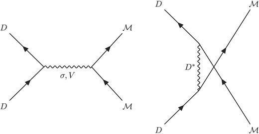
Feynman diagrams for the t and u channels. D and |$\mathcal {M}$| stand for the external charmed and light pseudoscalar mesons, respectively. |$\sigma$| and light vector mesons are exchanged in the t channel, whereas the vector charmed mesons are exchanged in the u channel.
Using the effective Lagrangians given above, we obtain the Feynman amplitudes as follows:
where |$p_i$| and |$k_i$| denote the inital and final four-momenta, respectively. The Mandelstam variables are defined as
We want to emphasize that any pole diagrams in the s channel are excluded, because we will explicitly show that |$D_{s0}^{*}$| and |$B_{s0}^{*}$| are dynamically generated. The values of the masses for the mesons involved in the current work are listed in Table 1, sourced from Particle Data Group data [27]. Note that, since the effects of isospin symmetry breaking are essential in the production of |$D_{s0}^{*}$|, we consider the isospin mass differences for the mesons involved.
Particle masses and spin-parity quantum numbers.
| Particle | Mass [MeV] | |$J^{PC}$| | Particle | Mass [MeV] | |$J^{PC}$| |
|---|---|---|---|---|---|
| |$\pi ^0$| | 134.98 | |$0^{-+}$| | |$D^0(\bar{D}^0)$| | 1864.84 | |$0^-$| |
| |$\eta$| | 547.86 | |$0^{-+}$| | |$D^\pm$| | 1869.66 | |$0^-$| |
| |$\sigma$| | 550 | |$0^{++}$| | |$D^{*0}(\bar{D}^{*0})$| | 2006.85 | |$1^-$| |
| |$\rho$| | 770 | |$1^{--}$| | |$D^{*\pm }$| | 2010.26 | |$1^-$| |
| |$\omega$| | 782.66 | |$1^{--}$| | |$D_s^\pm$| | 1968.35 | |$0^-$| |
| |$K^0(\bar{K}^0)$| | 497.611 | |$0^-$| | |$D_s^{*\pm }$| | 2112.2 | |$1^-$| |
| |$K^\pm$| | 493.677 | |$0^-$| | |||
| |$K^{*0}(\bar{K}^{*0})$| | 895.55 | |$1^-$| | |||
| |$K^{*\pm }$| | 891.67 | |$1^-$| |
Since the hadrons have finite sizes, we have to introduce the form factor at each vertex. We choose the following type of form factors:
where |$\Lambda$| stands for the cutoff mass and |$m_\mathrm{ex}$| designates the mass of the exchange meson. |$q^2$| is the squared momentum transfer between incoming and outgoing states. While a specific value of |$\Lambda$| depends on the size of a meson, we have no experimental and empirical information on it. The values of the cutoff masses bring about most of the uncertainties in any meson-exchange models because of the lack of experimental information on them. To reduce the uncertainties that may be caused by the cutoff masses, we utilize the idea that a heavier hadron is more compact than a light one [64–66], based on which we introduce a prescription that the value of |$\Lambda$| can be taken to be |$\Lambda \simeq (m_\mathrm{ex}+600)$| MeV. This was phenomenologically successful in describing various hadronic processes [40,41,58], in particular when heavy hadrons are involved [58,67]. We employ slightly smaller values of |$\Lambda$| (|$\Lambda \simeq (m_{\mathrm{ex}}+540)$| MeV) for the u-channel diagrams for locating the proper pole position. The dipole-type form factor |$n=2$| is used in this work. We list the cutoff parameters in Table 2.
The cutoff parameters in MeV for possible exchange diagrams for each reaction.
| Reaction | Exchange | Type | |$\Lambda -m_\mathrm{ex}$| [MeV] |
|---|---|---|---|
| |$D_s^+\pi ^0\rightarrow D_s^+\pi ^0$| | |$\sigma$| | t | 600 |
| |$D_s^+\pi ^0\rightarrow D_s^+\eta$| | |$\sigma$| | t | 600 |
| |$D_s^+\pi ^0(\eta )\rightarrow D^0K^+$| | |$K^{*+}$| | t | 600 |
| |$D^{*0}$| | u | 530 | |
| |$D_s^+\pi ^0(\eta )\rightarrow D^+K^0$| | |$K^{*0}$| | t | 600 |
| |$D^{*+}$| | u | 530 | |
| |$D^0K^+\rightarrow D^0K^+$| | |$\rho ^0$| | t | 600 |
| |$\omega$| | t | 600 | |
| |$D_s^{*-}$| | u | 540 | |
| |$D^+K^0\rightarrow D^+K^0$| | |$\rho ^0$| | t | 600 |
| |$\omega$| | t | 600 | |
| |$D_s^{*+}$| | u | 540 | |
| |$D^0K^+\rightarrow D^+K^0$| | |$\rho ^-$| | t | 600 |
The kernel matrix elements are then obtained as follows:
Since no neutral |$D_s^{*}$| state exists, the u-channel diagrams for the |$D^0K^+\rightarrow D^+K^0$| amplitude are absent. We will discuss this effect later. The |$D_s^+\pi ^0$| channel provides a background. The two |$DK$| channels play key roles in generating the |$D_{s0}^{*}(2317)$| resonance, while the |$D_s^+\eta$| channel shifts the pole position.
The matrix elements of |$\mathcal {V}$| are depicted in Fig. 2. We observe that the transition amplitudes |$\mathcal {V}_{D_s^+\pi ^0\rightarrow D^0K^+}$| and |$\mathcal {V}_{D_s^+\pi ^0\rightarrow D^+K^0}$| dominate over all other contributions, primarily due to the large coupling constants in the |$D^{*}$|-exchange diagrams in the u channel. The |$DK\rightarrow DK$| amplitudes provide significant contributions because of the large value of |$g_{DD^{*}\mathcal {M}}$| in the u channel. The |$D_s^+\eta \rightarrow DK$| amplitude contains the SU(3) symmetric factor of |$1/\sqrt{6}$|, which is smaller than that of |$1/\sqrt{2}$| for the |$D_s^+\pi ^0$| channel, as shown in Appendix A. Consequently, it gives a smaller contribution to the T-matrix. In the case of the |$D^0K^+\rightarrow D^+K^0$| amplitudes, no u-channel process is allowed due to the absence of neutral |$D_s^{*}$|. As a result, its contribution is expected to be marginal.
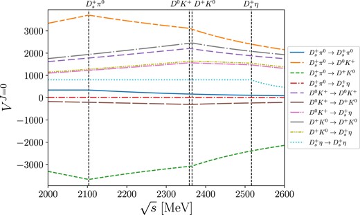
The partial-wave kernel amplitudes in four different channels. The dashed vertical lines represent the threshold energies for the channels involved in the current coupled-channel formalism.
We are now in a position to evaluate the coupled integral equations. The scattering amplitude is defined by
where |$P_i$| and |$P_f$| denote the total four-momenta of the initial and final states, respectively. We use the Blankenbecler–Sugar 3D reduction for the Bethe–Salpeter equations [48,49]:
The propagator |$G_k(q)$| takes the following form:
Defining the on-shell energies of particles 1 and 2 for the k channel, |$\omega _{1(2)}^k$|, as |$\omega _{1(2)}^k =\sqrt{\boldsymbol {q}^2+(m_{1(2)}^k)^2}$|, we obtain the Blankenbecler–Sugar (BbS) equations:
where
To generate the scalar |$D_{s0}^{*}(2317)$| meson dynamically, we only need the S-wave T amplitude, |$T^{J=0}$|. So, we carry out the partial-wave expansion of the BbS equation,
where |$V^J$| and |$T^J$| are the partial-wave kernel and transition amplitudes defined by
|$P_J(x)$| stands for the Legendre polynomial. Since Eq. (28) contains a singularity arising from the two-body propagator, we need to isolate the singular part as follows:
where the second term in the bracket is the singular part. |$\tilde{q}_k$| denotes the momentum point, where the singularity arises in the denominator. Constructing the off-shell partial-wave |$V^J$| and solving the partial-wave integral equation, we can derive the partial-wave |$T^J$|-matrix elements. Formally, the integral equation can be solved by using the matrix inversion:
Poles corresponding to resonance states can be found by evaluating the corresponding zeros of the equation |$\mathrm{det}(1-V^J(s)\tilde{G}^J(s))=0$|.
3. Results and discussion
We first examine the transition amplitudes |$T^{J=0}$| in the complex plane to see how the poles appear. To analyze the coupled-channel effects, we strictly follow our cutoff scheme |$\Lambda = (m_\mathrm{ex}+600)$| MeV for a while. Note that the kernel amplitudes do not contain any singularities because we do not include the s-channel diagrams. By solving the two-body integral equation with a single channel, we can identify which channels give rise to resonant states. Each T-matrix element is depicted in the left panel of Fig. 3. We see that the strong attraction in the u-channel exchange generates two poles in the |$D^0K^+$| and |$D^+K^0$| channels. Though the kernel amplitudes for the |$D_s^+\pi ^0\rightarrow DK$| and |$D_s^+\eta \rightarrow DK$| transitions also incorporate the u-channel diagrams, no poles appear in the corresponding T-matrix. Nevertheless, the |$D_s^+\pi ^0\rightarrow D^0K^+$| and |$D_s^+\pi ^0\rightarrow D^+K^0$| contributions show a significant enhacement at the |$D_s^+\pi ^0$| threshold energy. No pole structures were found in other T-matrix elements.
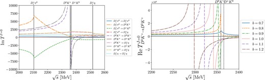
The real parts of the single-channel T-matrix elements are illustrated in the left panel, whereas in the right panel we show the effects of the u-channel diagrams in the single-channel integral equation with the parameter b varied from 0.7 to 1.2.
To investigate the channel effects, we introduce a parameter b to serve as a tool to illustrate the coupling between different channels and to demonstrate the emergence of poles in the complex plane, and multiply by it the coupling strength |$g_{DD^{*}\mathcal {M}}$|. Setting b to 0 turns off the corresponding channel, allowing us to observe the behavior when that particular channel is excluded. Conversely, setting b to 1 represents the full contribution of the transition matrix in the current work. In the right panel of Fig. 3, we depict the u-channel dependence of |$T_{D^0K^+\rightarrow D^0K^+}^{J=0}$| with b varied from |$b=0.7$| to |$b=1.2$|. Note that the pole, which arises from the strong attraction in the |$D^0K^+$| kernel amplitude, appears only if the value of b is approximately greater than 0.7. As anticipated, the energy corresponding to this pole increases as b becomes larger.
We now consider the S-wave transition amplitude for the |$D^0K^+ \rightarrow D^0K^+$| process. When the |$D^0K^+$| channel is coupled to the |$D^+K^0$| channel, the two poles still remain in the real |$\sqrt{s}$| axis below the |$D^0K^+$| threshold at |$\sqrt{s_R}=2322.04$| MeV and 2351.82 MeV, respectively, as depicted in Fig. 4. However, once we couple it to one of the nondiagonal amplitudes, only the first pole starts to undergo changes. For example, let us couple the |$D_s^+\pi ^0$| amplitude to the |$D^0K^+\rightarrow D^+K^0$| transition. We can scrutinize the coupled-channel effects by varying the coupling strength of the two channels, which is controlled by the parameter b. As b increases, the width of the first pole is rapidly broadened, as shown in Fig. 5. When b reaches 0.69, the deeper pole is already located at about |$\sqrt{s_R} \simeq 2110-i380$| MeV, which is very close to the |$D_s^+\pi ^0$| channel. Exceeding a value of |$b=0.7$|, this pole crosses the |$D_s^+\pi ^0$| threshold energy and subsequently disappears from the complex plane. By setting |$b=1$|, which corresponds to our final results, the first pole completely disappears. Consequently, we observe only the second pole, which remains largely unaffected by the |$D_s^+\pi ^0$| channel.
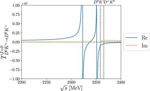
|$J=0$| partial-wave transition amplitude for the |$D^0K^+\rightarrow D^0K^+$| process when the |$D^0K^+$| and |$D^+K^0$| channels are coupled each other. The two poles lie below the |$D^0K^+$| threshold in the real axis.
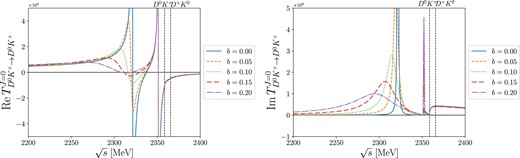
|$D_s^+\pi ^0$| channel coupled to the two |$DK$| channels. The real and imaginary parts of |$T_{D^0K^+\rightarrow D^0K^+}$| are depicted in the left and right panels, respectively. b varies from 0.00 to 0.20.
Next, we discuss how the |$D_s^+\eta$| channel comes into play. If we couple the |$D_s^+\pi ^0$|, |$DK$|, and |$D_s^+\eta$| channels together, the second pole starts to move to the lower energy, which is demonstrated in Fig. 6. When we introduce all possible coupled channels, the pole is finally positioned at approximately |$\sqrt{s_R}=(2261.4-i0.072)$| MeV.
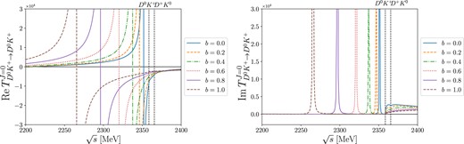
|$J=0$| partial-wave transition amplitude coupled to the |$D_s^+\eta$| channel with b varied from 0.0 to 1.0. The real and imaginary parts of |$T_{D^0K^+\rightarrow D^0K^+}$| are depicted in the left and right panels, respectively.
The pole position on the real axis |$\mathrm{Re}\, \sqrt{s_R} = 2261.4$| MeV still deviates from the experimental data for the mass of |$D_{s0}^{*}(2317)$|. Consequently, it is necessary to adjust the model parameters, with the uncertainties minimized. We itemize how we proceed to fit the |$D_{s0}^{*}(2317)$| mass:
We can slightly change the cutoff masses listed in Table 2.
While we still have one more free parameter, i.e. |$g_{\eta \eta \sigma }$|, its effect is almost negligible.
We can also consider the effects of the explicit flavor SU(3) symmetry breaking, but find that they are also negligible.
Thus, we try to fit the cutoff masses to ensure that the resulting values align with our prescribed criterion |$\Lambda \simeq (m_{\mathrm{ex}} + 600)$| MeV as far as possible. The cutoff masses for the exchanged light mesons, detailed in Table 2, are maintained at |$\Lambda = (m_{\mathrm{ex}} + 600)$| MeV in the t channel, while slightly smaller values are chosen for the exchanged heavy mesons in the u channel, specifically |$\Lambda \approx (m_{\mathrm{ex}} + 540)$| MeV. Ultimately, this fitting process leads us to the physical pole position situated in the second Riemann sheet: |$\sqrt{s_R} = (2317.90 - i0.0593)$| MeV, visually depicted in Fig. 7. The figure illustrates the pole corresponding to the |$D_{s0}^{*}(2317)$| meson in the complex plane. The pole for the |$D_{s0}^{*}(2317)$| meson is located approximately 40 MeV below the |$DK$| thresholds, which indicates that |$D_{s0}^{*}(2317)$| may be identified as a |$DK$| molecular state [17,18,20].
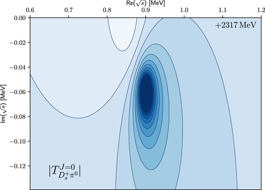
Contour plot of |$D_{s0}^{*}(2317)$|. The pole position is predicted as |$\sqrt{s_R} = (2317.90 - i0.0593)$| MeV.
To explore the effects of the coupled channels in more detail, we analyze the channel couplings for the channels involved. The transition amplitudes in the vicinity of the pole position |$\sqrt{s_R}$| can be parametrized as
The residue can be extracted by taking the limit |$s\rightarrow s_R$| as follows:
The channel coupling is defined by
which characterizes the coupling strength of the corresponding resonance with a given channel a. We predict the four different channel couplings as follows:
We can also define the corresponding coupling strengths:
Note that the channels corresponding to |$g_i$| (|$i=2,\, 3,\, 4$|) are not experimentally reachable by kinematics. The value of |$g_1$| is the predicted one, since all the parameters are fixed by reproducing the mass of the |$D_{s0}^{*}(2317)$| meson. Using the predicted value of |$g_1$|, we determine the |$D_{s0}^{*+}\rightarrow D_s^+\pi ^0$| decay width:
where |$\rho _{R}(s)$| stands for the two-body phase space factor and |$p_\mathrm{cm}$| denotes the center of momentum for the final states. The predicted value |$\Gamma _{D_{s0}^{*+}\rightarrow D_s^+\pi ^0} = 13.86\, \mathrm{keV}$| lies within the experimental upper limit of 3.8 MeV.
To scrutinize the reason for the very small value of the partial width, we investgate two significant sources of the decay width. One is the |$\pi ^0$|–|$\eta$| mixing effect discussed previously, while the other is the mass difference between neutral |$D^0$| (|$K^0$|) and charged |$D^+$| (|$K^+$|). If we neglect their mass differences, then we can specifically focus on the contribution of |$\pi ^0$|–|$\eta$| mixing to the decay width. Interestingly, we observe that the decay width becomes approximately doubled, i.e. |$\mathrm{Im} \sqrt{s_R} = -0.1070$| MeV, in comparison with the original results. This indicates that the |$\pi ^0\!-\!\eta$| mixing undergoes destructive interference from isospin effects arising from the mass differences between |$D^0$| (|$K^0$|) and |$D^+$| (|$K^+$|). Accordingly, the channel coupling |$g_1$| becomes |$1.21 \times 10^{-1}$| GeV, resulting in a partial decay width of |$\Gamma _{D_{s0}^{*+} \rightarrow D_s^+ \pi ^0} = 70.55$| keV.
The coupling strengths convey information on which channel is the strongest one. We conclude from the results in Eq. (36) that the |$DK$| channel is the most dominant one, and |$D_s^+\eta$| is the second most significant one. In Table 3, we compare the current results for the channel couplings with those from other works. Interestingly, the values of the |$DK$| and |$D_s^+\eta$| coupling strengths from the present work are much larger than those from other works.
Comparison with different models.
Comparison with different models.
In the same theoretical framework, our analysis expands to include the scalar bottom-strange meson. Specifically, we employ the coupled-channel formalism to delve into the |$\bar{B}\mathcal {M}$| interaction with a positive strangeness, |$S=+1$|. It is crucial to highlight a distinction from the charm sector; the charged |$B_s^{*}$| meson is absent in the u-channel process of the |$B^-K^+$| channel. This means that the u-channel contribution to the bottom sector becomes smaller than that to the charm sector. To compensate this absence, we prefer to use a lower value of the cutoff mass for |$B_s^{*0}$|. So, we use the following values of |$\Lambda _{B^{*}}=(m_{B^{*}} + 630)$| MeV and |$\Lambda _{B_s^{*}}=(m_{B_s^{*}} +390)$| MeV. Note that if we adhere to 600 MeV for the difference between the mass of the exchanged particle and its cutoff value, then |$B_{s0}^{*}$| would not emerge as a molecular state in the present scheme. The pole for |$B_{s0}^{*}$| reappears in the second Riemann sheet, positioned at |$\sqrt{s_R} =(5756.43 - i0.0215)$| MeV, as visually represented in Fig. 8. It is noteworthy that the total width of the |$B_{s0}^{*}$| resonance, denoted as |$\Gamma _{\bar{B} {s0}^{*}}$|, exhibits a comparable value to that of the |$D_{s0}^{*}$| resonance. This observation is natural when considering that the two-body phase space factor, |$\rho _{\bar{B}_{s}^{0}\pi ^0}(m_{\bar{B}_ {s0}^{*}}^2)$| for the |$\bar{B}_{s0}^{*}$| resonance, is approximately two times smaller than that for |$D_{s0}^{*}$|.
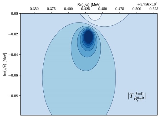
Contour plot of the |$\bar{B}_{s0}^{*}$| state. The predicted pole position is |$\sqrt{s_R} = (5756.43 -i0.0215)$| MeV.
We exmaine the channel couplings for the bottom-strange meson as follows:
The corresponding coupling strengths are given by
In the bottom sector, the |$BK$| channel is the most dominant one. As previously discussed, the strength of the |$B^-K^+$|-channel coupling is smaller than that of the |$\bar{B}^0K^0$| channel due to the absence of the u-channel diagram in |$B^-K^+$|. Furthurmore, the value of |$g_4$| is smaller than that of |$g_2$| and |$g_3$| for the same reason. Since we use smaller values of the cutoff masses, we want to mention that the present finding does not guarantee the existence of |$\bar{B}_{s0}^{*}$|. However, if it is found by an experiment, we can get a hint that the structure of |$B_s^{*}$|, which brings about the main contribution, is different from other heavy mesons considered in the current theoretical description, and |$\bar{B}_{s0}^{*}$| is also understood as a molecular state.
4. Summary and conclusions
In the current work, we aimed to investigate |$D_{s0}^{*}(2317)$|, studying |$D_s^+\pi ^0$| scattering within the off-shell coupled-channel formalism. We introduced four different coupled channels in the charge basis: |$D_s^+\pi ^0$|, |$D^0K^+$|, |$D^+ K^0$|, and |$D_s^+\eta$|, with positive strangeness |$+1$|. We first constructed the invariant kernel amplitudes based on the effective Lagrangians derived from heavy-quark effective theory and hidden local symmetry. Having inserted the kernel amplitudes into the Blankenbecler–Sugar-type coupled integral equations, we evaluated the transition amplitudes. Since |$D_{s0}^{*}(2317)$| is the scalar meson, we carried out a partial-wave expansion to pick out the S-wave transition amplitude. We then scrutinized the |$DK$| channels for how the pole appears dynamically. When we only considered the |$DK$| channels, two poles emerged. Adding different channels one by one, the width of the first pole became broadened. Once we included all the coupled channels, the first pole disappeared, and at the same time the position of the second pole started to move to lower energies. Having fitted the cutoff masses, the pole is positioned at the physical mass of |$D_{s0}^{*}(2317)$|. The |$D_{s0}^{*}\rightarrow D_s^+ \pi ^0$| decay width was predicted to be 13.86 keV, which lies within the experimental upper limit. The |$DK$| channels were found to be the most dominant. We observed that the two sources of the decay width interfere destructively with one another. This leads to a small value of the partial decay width of |$D_{s0}^{^+}\rightarrow D_s^+\pi ^0$|. |$D_{s0}^{*}$| is positioned below the |$DK$| threshold, indicating that it can be interpreted as the |$DK$| molecular state. On the other hand, the generation of |$\bar{B}_{s0}^{*}$| requires a smaller value of the cutoff mass due to the absence of the charged |$B_s^{*}$|-exchange process. Thus, the existence of |$\bar{B}_{s0}^{*}$| is less evident than that of |$D_{s0}^{*}$|.
Acknowledgement
We are very grateful to Samson Clymton for useful comments and discussion.
Funding
The present work was supported by the Basic Science Research Program through the National Research Foundation of Korea funded by the Korean government (Ministry of Education, Science and Technology, MEST), Grant Nos. 2021R1A2C2093368 and 2018R1A5A1025563. Open Access funding: SCOAP3.
Appendix A. SU(3) relations
We provide the flavor SU(3) relations for the coupling constants for the |$HH\mathcal {M}$| and |$HHV$| vertices:
and
For the |$\mathcal {M}\mathcal {M}\mathcal {M}$| and |$\mathcal {M} \mathcal {M}V$| vertices, we have
