


Abstract
We have been developing a high-pressure xenon gas time projection chamber (TPC) called AXEL (A Xenon ElectroLuminescence detector) to search for neutrinoless double-beta (0νββ) decay of 136Xe. The unique feature of this TPC is the electroluminescence light collection cell (ELCC), the part designed to detect ionization electrons. The ELCC is composed of multiple units, and one unit covers 48.5 cm2. A 180 L size prototype detector with 12 units, 672 channels, of the ELCC was constructed and operated with 7.6 bar natural xenon gas to evaluate the performance of the detector around a Q value of 136Xe 0νββ. The obtained FWHM energy resolution is |$0.73 \pm 0.11\%$| at 1836 keV. This corresponds to |$0.60 \pm 0.03\%$| to |$0.70 \pm 0.21\%$| of the energy resolution at a Q value of 136Xe 0νββ. This result shows the scalability of the AXEL detector with the ELCC while maintaining a high energy resolution. Factors determining the energy resolution were quantitatively evaluated and the result indicates that further improvement is feasible. Reconstructed track images show distinctive structures at the endpoints of electron tracks, which will be an important feature in distinguishing 0νββ signals from gamma-ray backgrounds.
1. Introduction
Whether neutrinos have a Majorana nature is key to resolving the problems of the light neutrino masses [1–3] and the matter–antimatter asymmetry of the universe [4]. The most practical way considered so far to confirm the Majorana nature of neutrinos is to search for neutrinoless double-beta (0νββ) decay [5,6]. The current most stringent limit was obtained with the 136Xe nucleus; the KamLAND-Zen experiment set the lower limit of the half-life to be 2.3 × 1026 years (90% C.L.) [7].
More sensitive searches for 0νββ require a large target mass over a ton scale, ultra-low radioactivity in the surrounding materials, and powerful discrimination between signals and backgrounds. In the case of 136Xe, 2ν-emitting double-beta decay (2νββ) and gamma rays from 214Bi (2448 keV) and 208Tl (2615 keV) would be severe sources of backgrounds because they have energy close to the Q value of 0νββ (2458 keV). A high energy resolution is therefore essential for signal–background discrimination. Detection of the event pattern is also important because 0νββ has one cluster with two thick endpoints corresponding to two beta rays, whereas a gamma-ray event has multiple clusters or only one thick endpoint. A high-pressure xenon gas time projection chamber (TPC) has the potential to achieve these requirements. The application of high-pressure xenon gas TPCs for 0νββ searches began with the Gotthard experiment [8,9]. Now, there is leading research by the NEXT experiment [10], and the PandaX-III experiment [11] is also pursuing studies.
We have also been developing a high-pressure xenon gas TPC called AXEL (A Xenon ElectroLuminescence detector) to search for 0νββ. A peculiar feature of the AXEL detector is the unique ionization-electron counting technique using electroluminescence (EL), called the electroluminescence light collection cell (ELCC). We demonstrated the proof-of-principle of the ELCC in Ref. [12] and showed an energy resolution of |$1.73\pm 0.07\%$| (FWHM) for 511 keV electrons in Ref. [13]. In this paper, we describe the performance around the Q value of 136Xe 0νββ, 2458 keV, with a larger-scaled AXEL prototype detector.
2. Detector
A schematic view of the AXEL detector is shown in Fig. 1. High-energy charged particles deposit their energies by exciting and ionizing xenon atoms along with the tracks. Excited atoms emit primary scintillation lights on timescales of hundreds of nanoseconds, and they are detected by photomultiplier tubes (PMTs) at the cathode side. Ionization electrons drift under the uniform electric field made by the field cage and are converted to photons and detected by the ELCC at the anode side on timescales of tens of microseconds. The energies deposited by the charged particles are reconstructed from the photon counts at ELCC. The tracks of the charged particles are reconstructed from the hit pattern on the ELCC and the time difference between the hits on the PMTs and ELCC. A large-area ELCC is composed of multiple units.
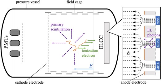
Schematic view of the AXEL 180 L prototype detector.
A 180 L prototype detector with three 48.5 cm2 ELCC units was constructed and evaluated in Ref. [13]. Since then, the sensitive volume of the detector was enlarged and the structure of the ELCC was improved.
2.1. Electroluminescence light collection cell
The ELCC is a pixelized detector for ionization electrons. It consists of the TPC-anode electrode, a ground potential mesh electrode, and a polytetrafluoroethylene plate (PTFE body) in between them. The anode electrode and PTFE body have holes (“cells”) arranged in a hexagonal lattice pattern. An electric field up to 3 kV/cm/bar, which is produced by the anode and mesh electrode and 30 times more intense than the drift field, draws ionization electrons into these cells and accelerates them. At this field, electrons excite but not ionize xenon atoms. EL photons are generated by the deexcitation of these atoms. For each cell, VUV-sensitive silicon photomultipliers (Hamamatsu MPPC, S13370-3050CN) are placed behind the mesh electrode and detect the EL photons (see Fig. 1). The advantages of the ELCC are the following two points. One is that the number of detected photons is less dependent on the initial position of the ionization electrons because the EL process occurs after the ionization electrons are drawn into cells. The other is that there is little deformation of electrodes because the structure is supported by the PTFE body.
The plane of the ELCC is made of parallelogram-shaped units of 56 (= 7 × 8) channels each. The fundamental dimensions of the ELCC are optimized [13] for the drift field of 100 V/cm/bar and the EL field of 3 kV/cm/bar, i.e.,
anode hole diameter: 5.5 mm
PTFE body hole diameter: 4.5 mm
cell depth: 5 mm
cell pitch: 10 mm
A cross-sectional view of the ELCC plane with the previous setup adopted in Ref. [13] is shown in the upper part of Fig. 2.
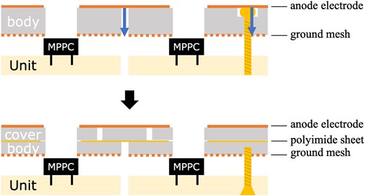
Schematic cross-sectional views of the ELCC structures. The previous structure is shown in the upper part and the upgraded structure to prevent discharges is shown in the lower part. The paths of discharges are shown by the blue arrows in the upper part.
Frequent and severe electric discharges occurred when the operating voltage was increased together with an increase in the operating pressure from 4 to 7.6 bar. The discharges occurred between the anode and the ground mesh electrodes at the boundaries of the ELCC units and the screw holes to fix the ELCC units. We have applied the following countermeasures to prevent these discharges. First, the PTFE body is separated into two layers. We call the upper (the anode electrode side) layer the “cover”. The shape of the cover was changed from that of the units to shift the boundaries from those of the lower layers. Then, the anode electrode and the ground mesh electrodes do not face each other directly. A |$125 \,\mathrm{{\mu }m}$| polyimide sheet is inserted between the two layers to block the intersection of the boundaries (see Fig. 3). Second, the direction of the screws to fix the ELCC units is reversed so that there are no holes going through the ELCC units. These two countermeasures are illustrated in the lower part of Fig. 2. Lastly, the mesh electrodes are covered by two perfluoroalkoxyalkane (PFA) films so as not to expose sharp edges that trigger corona discharges (see Fig. 4). This also prevents the mesh from fraying, and it suppresses discharges caused by mesh fragments getting into the cells. The PFA films have holes corresponding to the cells to prevent charge-up.
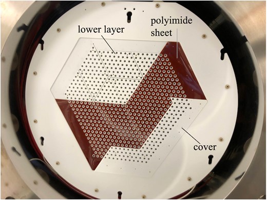
Photograph of the upgraded ELCC plane during assembly. Part of the polyimide sheets and the covers have been removed.
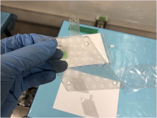
Photograph of the mesh electrode welded between PFA films.
Together with these countermeasures, the number of ELCC units was increased from 3 to 12, and the total number of channels is 672, to observe the events with higher energies and longer tracks. The sensitive area is around 580 cm2.
The signals of MPPCs are transferred via cables of flexible printed circuits (FPCs) and recorded with dedicated front-end boards AxFEB [14] at 5 MS/s for each unit. The bias voltages for the MPPCs are also supplied by the same FPC cables.
2.2. Field cage
An intense and uniform drift electric field is necessary to achieve a high energy resolution and fine track image since it suppresses the fluctuation of recombination, attachment, and diffusion of ionization electrons during the drift. In contrast, the collection efficiency of the ionization electrons into the ELCC cells decreases if the drift field is not sufficiently low compared to the EL field. We adopted 100 V/cm/bar for the drift field as a design value with allowed deviations of ±5%. The energy resolution is expected to get worse below 100 V/cm/bar because of the recombination of ionization electrons [15].
The field cage to generate the drift field consists of 3 mm thick and 12 mm wide band-shaped aluminum electrodes aligned between the anode and the cathode electrodes. They have two different diameters (505 mm and 489 mm) and are alternately lined up with an overlap of 1 mm to shield the effect of the ground potential of the pressure vessel. The inner diameter of the pressure vessel is 547 mm. The vessel and the outer electrodes are insulated by a 20 mm thick high-density polyethylene (HDPE) cylinder. Each ring electrode has a straight section of 300 mm to allow cabling space between the HDPE cylinder and the field cage. A cathode mesh electrode is placed on top of the ring electrode array. The mesh is point-welded to a 1 mm thick stainless steel frame under tension, and thus deflection of the mesh is kept small. Negative high voltage is applied to the cathode mesh via a wire covered by silicone rubber. The cathode, ring electrodes, and anode are connected in series via 100 MΩ resistors to equally apply potential differences between neighboring electrodes. Six pillars made of polyetheretherketone (PEEK) support the electrodes from the inside. The ends of the pillars are fixed to the PTFE disk hosting the anode plane. Figure 5 shows a photograph of the field cage.
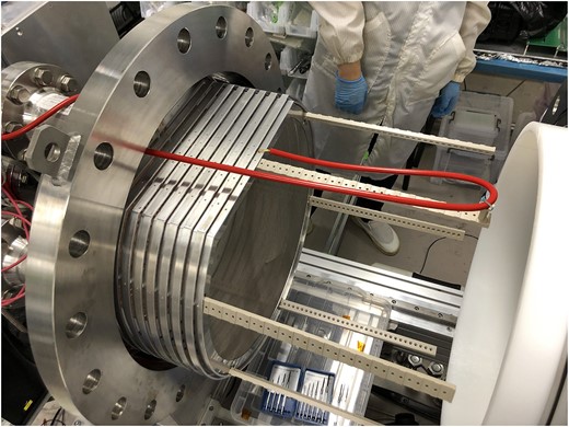
Photograph of the field cage installed in the pressure vessel. The white cylinder on the right side is the HDPE insulator.
A finite element method calculation by FEMM [16] on this configuration showed that the intensity of the drift field satisfies 100 V/cm/bar ± 5% in the region within 229.3 mm from the central axis. The sensitive area of the 12-unit ELCC is fully inside this uniform region.
The distance between the cathode mesh electrode and the anode plane, the drift length, is adjustable up to 46 cm. Due to the limitation of the cathode high-voltage supply, however, it was limited to 18 cm in this paper. The sensitive volume is about 10 000 cm3 as a result.
2.3. PMTs
We use VUV-sensitive and high-pressure-tolerant PMTs, Hamamatsu R15298. The number of PMTs to detect primary scintillation lights is increased to seven from two in the previous paper [13]. They are mounted behind the cathode mesh at a large enough distance so as not to cause an intense electric field over the EL threshold even if the field cage is fully extended to 46 cm. The resulting distance between PMTs and the cathode mesh this time is approximately 38 cm. A guard mesh at the ground potential is placed in front of the PMTs. The number of photons reaching the PMTs is decreased by the aperture ratio of the two meshes, 71% for the cathode mesh and 67% for the guard mesh.
The signals of PMTs are transferred via PTFE-coated coaxial cables, amplified 100-fold with fast amplifiers, and recorded by a 100 MS/s waveform digitizer (CAEN, v1724).
3. Measurement
To evaluate the performance of the upgraded detector around the Q value of 136Xe 0νββ, we conducted measurements with gamma-ray sources. The measurement conditions and procedure are described below.
Before introducing xenon gas into the pressure vessel, an evacuation was conducted for two weeks. The vacuum level reached 3.9 × 10⁻² Pa, and the outgassing rate was 1.23 × 10⁻⁴ Pa m3/s. After the evacuation, 7.6 bar of natural xenon gas was added, and the gas was circulated with a flow of 5 NL/min and purified by a molecular sieve (Applied Energy Systems, 250C-V04-I-FP) and a getter (API, API-GETTER-I-RE). Before starting the measurement, we undertook three weeks of purification while monitoring the improvement of the EL light yield.
The intensities of the EL and drift electric fields were 2.5 kV/cm/bar and 83.3 V/cm/bar, respectively. These are lower than the design values of 3 kV/cm/bar and 100 V/cm/bar. This is because frequent discharges still occurred at the ELCC at the design value. The ratio between the EL and drift field intensity was kept at 0.1:3 to maintain 100% collection efficiency of ionization electrons into the ELCC cells. The applied high voltages were hence −9.5 kV for the anode and −20.9 kV for the cathode. At these conditions, discharges took place once every several hours on both the anode and cathode. When a discharge occurs, an interlock system cuts off the high voltages, and they are reapplied manually.
Two kinds of gamma-ray sources were used. One is an 88Y source, which mainly emits gamma rays of 898.0 keV and 1836 keV. The intensity of the source was 9 kBq. The other is a set of thoriated tungsten rods. They are commercial products for welding and include 2% of thorium by mass. Thus they can be used as a source of thorium series radiations including 2615 keV gamma rays of 208Tl. The amount of thoriated tungsten rods used was 1 kg, resulting in 80 kBq of intensity. The source was set at the outside surface of the pressure vessel during the measurement.
Data were taken for five days for 88Y and one day for thoriated tungsten rods in June 2022 with intervals for commissioning and data checking. The anode and cathode voltages, gas pressure, gas temperature, water concentration, etc. were monitored during the data taking. Figure 6 shows the trends in important monitor values.
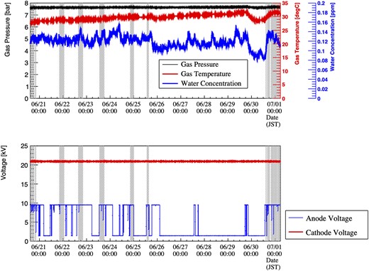
Trends in the monitor data. The upper panel is for gas conditions, and the lower panel is for high voltages. The gray-shaded areas are data-taking periods. The drop in the anode voltage corresponds to discharges or manual off.
The outermost 87 channels out of 672 channels of the ELCC were assigned to the veto. Apart from that, there was one channel with a high dark current and one dead channel. The high dark-current channel and six channels around the dead channel were also added to the veto (see Fig. 7).
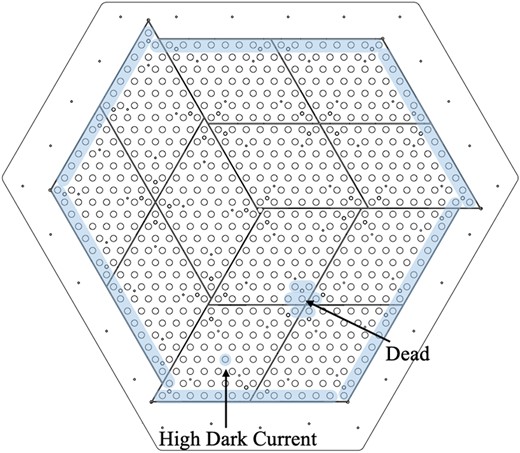
Configuration of veto channels. The blue-shaded channels were assigned to veto.
Two kinds of triggers were used for the data acquisition of the ELCC signal. One is called a fiducial trigger, which is issued when the sum height of the signal of channels other than the predefined veto channels exceeds a threshold, and the veto channels have no hits. The threshold of the fiducial trigger was set around 400 keV. The other, the whole trigger, sets a threshold on the signal sum for all channels including the veto channels. It is to take calibration data targeting 30 keV characteristic X-rays and was prescaled to 1/50.
To issue the triggers, a trigger board, a Hadron Universal Logic module (HUL) [17], is used. Each FEB sends the waveform to HUL, and HUL sends the trigger and veto signal and a common 160 MHz clock to FEBs. HUL outputs two other NIM signals. One is called the send-trigger signal, which is synchronized with the trigger to FEBs. The other is called the send-header signal, which is synchronized with the timing of data transmission to the DAQ PC after waveform acquisition at FEB is complete.
The data acquisition of the PMT signal is triggered by the send-header signal from HUL. The waveform recording window is set to |$600 \,\mathrm{\mu s}$|, and the pre-trigger region is 95% of the window so that the timing of primary scintillation is certainly included in the window. The waveform digitizer for PMTs also records the send-trigger signal from HUL, and the signals were used to match the timing of the corresponding events of the ELCC and PMTs.
The number of total acquired events is 1145 761 for the 88Y run and 869 422 for the thoriated tungsten rod run. We used the whole dataset to evaluate the detector performance.
4. Analysis
The analysis process is composed of three steps.
The first is the ELCC waveform analysis (Sect. 4.1), which consists of the search for hits, clustering, correction to the non-linearity of MPPCs, and correction to the gain of the EL process in each ELCC cell. From this step, we can estimate the number of ionization electrons, the energy, or the track pattern.
The second is the PMT waveform analysis (Sect. 4.2), which consists of the search for PMT hits, identification of the primary scintillation, and matching to the ELCC events. From this step, we can determine the time of the event relative to the ELCC signal and hence the absolute position of each ionization along the direction of the drift (hereafter, the z-position).
The last step is overall cuts and corrections (Sect. 4.3).
The same analysis method was used for both the 88Y run and the thoriated tungsten rod run; however, the correction coefficients are different for each run.
4.1. ELCC waveform analysis
Figure 8 shows typical waveforms of the ELCC signal.
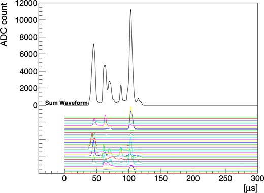
Typical waveforms of the ELCC signal. The waveform of each channel is shown by colored lines with arbitrary offsets. The sum of the waveforms is shown by the black line.
Hits are searched for a threshold of 3.5 ADC counts above the baseline, which corresponds to 3.8 photons equivalent. The rise timing and the fall timing of a hit are defined as the threshold-crossing timing. From the five samplings before the rise timing to the five samplings after the fall timing, the ADC counts of the waveform are summed up, and the sum is converted to the photon count by using the gain of the channel’s MPPC. The gains are pre-calculated using the MPPC’s dark current pulses, as described in Refs. [12,14].
Hits that are in adjacent channels and overlapped in time are identified as belonging to the same single cluster. All hits in an event are assigned to clusters.
Events are removed from further analysis if ADCs overflow, the rise timing is less than 20 samplings (|$4 \,\mathrm{\mu s}$|), or the fall timing is over 1300 samplings (|$260 \,\mathrm{\mu s}$|).
4.1.1. MPPC non-linearity correction
MPPCs have a non-linear output for high incident light intensity. This is because the number of MPPC pixels is limited, and it takes a finite time for each pixel to restore the bias voltage after the charge is released by photon detection. Thus, the non-linearity is characterized by the number of pixels and recovery time and is corrected with the following equation [13]:
where Nobserved and Ncorrected are the photon counts before and after the correction, respectively; τ is the recovery time; Δt is the time width applying this correction, 200 ns in this analysis corresponding to the sampling speed of the FEBs; and Npixel = 3600, the number of pixels.
The recovery times of each MPPC were measured in advance by measuring the responses to the high-intensity LED light. To monitor the true number of photons incident to MPPCs, one MPPC with a 5% ND filter attached was used as a reference. The mean of the measured recovery times is 73.4 ns. Figure 9 shows the distribution of the measured recovery times.
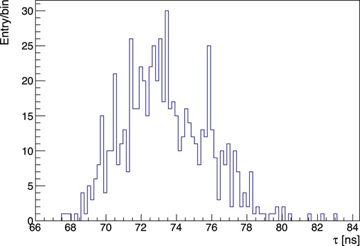
Distribution of the measured recovery times of MPPCs.
4.1.2. EL gain correction
The gain of the EL process in each ELCC cell (hereafter, EL gain) is defined as the mean of the detected photon count when one ionization electron enters the cell. The EL gains are different channel by channel due to dimensional differences from machining accuracy, differences in the photon detection efficiency of MPPCs, and so on. Thus, each signal should be corrected using its gain relative to the mean over channels to obtain better energy resolution.
The correction factors are determined by using the peak of Kα characteristic X-rays (29.63 keV) in the photon count spectra. To conduct this, clusters in which the target channel has the highest photon counts are used. Throughout this procedure, the correction factors of the adjacent channels affect the determination of the correction factor of the channel. Hence this procedure is applied to all channels and iterated multiple times until the factors converge: in this analysis, six times.
The mean of the EL gains is 12.5 photon/electron for this measurement.
4.2. PMT waveform analysis
Figure 10 shows typical signal waveforms of the PMTs. Very narrow hits coinciding in two PMTs and preceding the EL signals are the primary scintillation photon candidates.
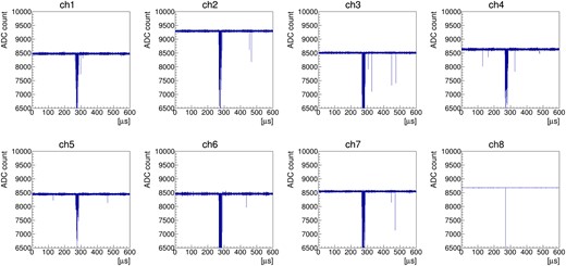
Typical waveforms of the PMTs. The hits at ∼|$130 \,\mathrm{\mu s}$| in channel 4 and channel 5 are the scintillation signals. The hits around |$300 \,\mathrm{\mu s}$| are EL from the ELCC. Channel 8 records the send-trigger signal from HUL as mentioned in Sect. 3, not the PMT signal.
The hit threshold is set at 200 ADC counts below the baseline. It is sufficiently higher than noise and lower than 1 p.e. wave height. To separate hits by scintillation light from hits by EL lights, hits are selected when they have a width less than 400 ns and are more than |$1 \,\mathrm{\mu s}$| apart from other hits. Hereafter, hits selected by this criterion are called scintillation-like hits, and the others are called EL-like hits. Of these scintillation-like hits, those that are coincident within 100 ns in two or more channels are reconstructed as a hit cluster by the primary scintillation light. In cases where there are two or more hit clusters, such events are cut because it is not possible to determine which hit cluster is the actual primary scintillation.
The corresponding ELCC event and PMT event are matched based on the information of the timestamp and the internal clock of the ELCC FEBs and the PMT digitizer. For matched events, the time interval between the primary scintillation and the ELCC hits is calculated with the help of the send-trigger signal from HUL, which corresponds to the fixed timing in the data acquisition window for the ELCC. Figure 11 shows the distribution of the time intervals between the primary scintillation and the fall timing of the ELCC events. The peak in this distribution corresponds to the cathode plane of the field cage; in other words, z = 18 cm. From this, the drift velocity of ionization electrons was derived to be |$1.04 \,\mathrm{mm}/\mathrm{\mu s}$|. Using this drift velocity, the z-position of each ionization signal detected by the ELCC is reconstructed.
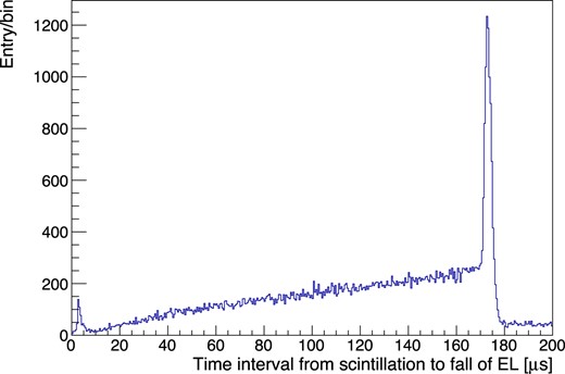
Distribution of the time intervals between scintillation and the fall timing of the ELCC events. The peak at |$175 \,\mathrm{\mu s}$| is formed by the events across the cathode plane.
4.2.1. Selections to avoid timing mismatch
Events are cut when there are multiple send-trigger signals from HUL because it leads to a timing mismatch depending on which one corresponds to the true beginning of the ELCC events. This can be caused by the pile-up of events during the drift of ionization electrons.
Events with EL-like hits within the 18 cm-equivalent time preceding the ELCC signal are cut. Finally, events are cut if there exist scintillation-like hits, even a single hit without any coincidence, in the region corresponding to within 2 cm from the ELCC signal. This is because ionization electrons generated within 2 cm of the ELCC surface are not guaranteed to have 100% collection efficiency into the ELCC [13]; thus the energy resolution gets worse if it fails to cut events whose actual rising edge is within 2 cm.
4.3. Fiducial volume cuts and overall corrections
Using the information obtained from the ELCC and PMT signal analysis, fiducial volume cut and overall corrections are applied.
4.3.1. Elimination of clusters with small photon counts
Many events contain a few to several tens of clusters with photon counts of less than one hundred. These clusters are generated from one to a few electrons. Figure 12 shows the distribution of the photon counts and the drift distance after the rising of the ELCC signal for these small photon count clusters. The dense region around 180 mm, which corresponds to the length of the drift region, is considered to be clusters by electrons generated by VUV EL light hitting the cathode mesh. The other clusters can be formed in the same manner with various detector components and also by the ionization electrons that attach to impurities in the gas during drift and are released after a while. Such a phenomenon is also observed in liquid xenon detectors [18–20].
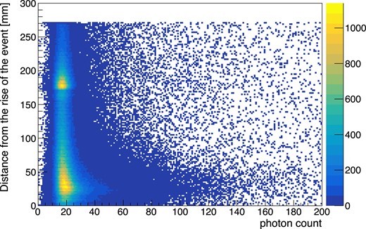
Drift distance after the rising of the event and photon counts for the clusters with small photon counts.
Because these clusters with small photon counts disturb the fiducial cut (Sect. 4.3.2) and reconstruction of tracks, the clusters with less than 100 photons are eliminated from events. The total photon counts of eliminated clusters are 400 photons at maximum for each event. Thus the effect on the reconstruction of energies is less than 0.04% for the 1836 keV photopeak and negligible compared to the energy resolution.
4.3.2. Fiducial volume cut
Fully contained events are selected by rejecting events that have any hits on veto channels (Sect. 3) and events whose z-position extends beyond the 2 cm < z < 17.5 cm region.
4.3.3. Correction of time variation
Figure 13 shows the time variation of photon counts of clusters around the energy of the Kα characteristic X-ray. The cause of variation can be changes in the gas conditions: temperature, density, and purity. The correction factors are derived for divisions every 30 minutes. The width of the time bin, 30 minutes, is determined so that the width of the peak of 1836 keV is minimized, balanced between the statistical error of the correction factor and the sensitivity to the time variation.
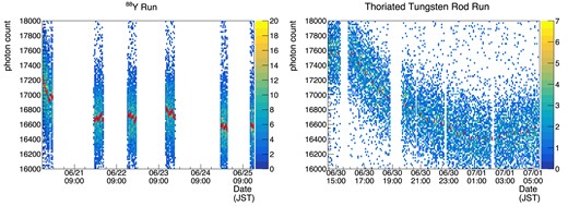
Variation of photon counts with time. The points with error bars represent the mean of the Kα peak in each time division. The left panel is for the 88Y run and the right is for the thoriated tungsten rod run.
4.3.4. Correction of z-dependence
Some of the ionization electrons are not detected because of the attachment by impurities during drift. This attenuation is characterized by the following equation:
where N0 and N(z) are the photon counts before and after the attachment respectively and λ is the attenuation length. Figure 14 shows the dependence of the photon counts of Kα clusters on the z-position. From this dependence, attenuation lengths of λ = 21 700 + −3700 mm for the 88Y run and λ = 17 000 + −2700 mm for the thoriated tungsten rod run were obtained. These correspond to electron lifetimes of 20.9 + −3.6 ms and 16.3 + −2.6 ms respectively. Using these attenuation lengths, the photon counts are corrected for every sampling of the waveforms.

Dependence of the photon counts of Kα clusters on the z-position for the 88Y run. The red line shows the fitted function.
4.3.5. Overall fine-tuning for the recovery times of MPPCs
As described in Sect. 4.1.1, the non-linearity of the MPPCs is corrected using the recovery times of MPPCs measured in advance. However, the effective recovery times can vary depending on the conditions of the MPPCs, such as temperature, or shadow of the mesh electrode in front of the MPPCs. The deviation in photon counts due to the difference between the true recovery time and the measured recovery time can be expressed as follows:
where Ntrue is the true total photon count of the event, i runs for every sampling of the waveform of every hit channel, |$N_\mathrm{obs}^i$| and |$N_\mathrm{rec}^i$| are the photon counts for each sampling of the waveform before and after the MPPC non-linearity correction, respectively, ri is the correction factor other than the MPPC non-linearity, |$k^{\left(^{\prime }\right)} = \tau ^{\left(^{\prime }\right)}/\left(\Delta t \cdot N_\mathrm{pixel}\right)$|, |$\tau ^{\left(^{\prime }\right)}$| is the true (measured) recovery time of the channel, and Δk = k − k′. The last line assumes that Δk is small and common among channels. This equation indicates that, if there exists an overall bias in the recovery times, it appears as a slope of the relation between the photon counts and |$\sum _ir^i\left(N_\mathrm{rec}^i\right)^2$| (hereafter called the corrected squared sum, CSS).
Figure 15 shows the distribution of the photon counts and the CSS. To determine the Δk and corresponding biases of the MPPC recovery times, peaks with sufficient statistics are used: the photopeak of 898 keV gamma rays and the double escape peak of 1836 keV gamma rays for the 88Y run, and the photopeak of 583 keV gamma rays and the double escape peak of 2615 keV gamma rays for the thoriated tungsten rod run. From the slope at each peak of the photon counts, the biases for the MPPC recovery times were derived as +2.35 ns for the 88Y run and +3.13 ns for the thoriated tungsten rod run.
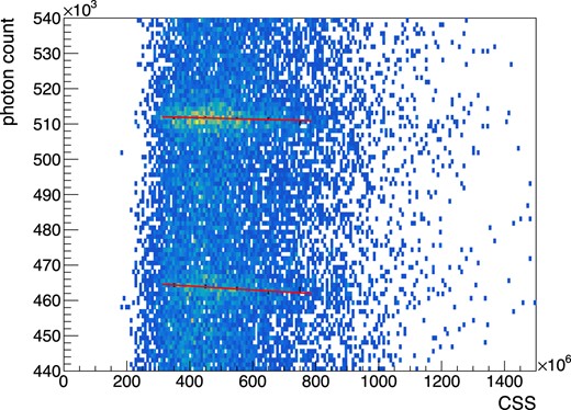
Relation between the photon counts and the CSS for the photopeak of 898 keV gamma rays (∼5.1 × 10⁵ photon) and the double escape peak of 1836 keV gamma rays (∼4.6 × 10⁵ photon) in the 88Y run.
The MPPC non-linearity correction, EL gain correction, time variation correction, and z-dependence correction are repeated with the recovery times shifted by these biases.
5. Detector performance
From the analysis in the previous section, the EL photon count and track of events are obtained. Based on these, we evaluate the performance of the detector.
5.1. Energy resolution
Figure 16 shows the EL photon count spectra of each run. Several peaks are identified in the spectra: peaks of characteristic X-rays of xenon, full peaks of gamma rays from the sources and environment, and double escape peaks of pair creation. Each peak was fitted assuming a Gaussian peak and linear background. For the gamma-ray full peaks, single-cluster events and multi-cluster events were fitted separately. Figure 17 shows an example of the fit results, and Table 1 is the summary.
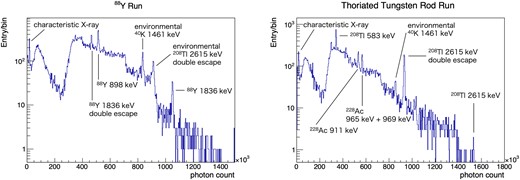
Photon count spectra after all of the corrections and cuts. The left panel is for the 88Y run and the right is for the thoriated tungsten rod run. The dip around 200 photon count corresponds to the threshold of the fiducial trigger.
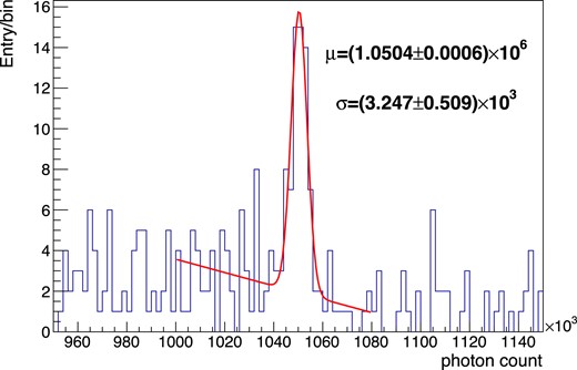
Result of the fit to the spectrum of the single-clustered full energy peak of 88Y 1836 keV gamma rays.
Summary of the peak fit result. SS stands for single-site events and MS stands for multiple-site events for gamma-ray full peaks. 40K multi-cluster events in the thoriated tungsten rod run were too few to evaluate the resolution.
| Energy | Mean photon counts | Resolution [FWHM] | |
|---|---|---|---|
| 88Y run | |||
| Kα | 29.68 keV | (1.6870 ± 0.0004) × 104 | |$(4.389 \pm 0.050)\%$| |
| Kβ | 33.62 keV | (1.9166 ± 0.0011) × 104 | |$(4.722 \pm 0.125)\%$| |
| Double escape of 88Y 1836 keV | 814.1 keV | (4.6512 ±0.0022) × 105 | |$(1.194 \pm 0.102)\%$| |
| 88Y SS | 898.0 keV | (5.1374 ±0.0022) × 105 | |$(1.152 \pm 0.119)\%$| |
| 88Y MS | |$(1.386 \pm 0.109)\%$| | ||
| Environmental 40K SS | 1461 keV | (8.3458 ±0.0042) × 105 | |$(0.81 \pm 0.11)\%$| |
| Environmental 40K MS | |$(1.09 \pm 0.16)\%$| | ||
| 88Y SS | 1836 keV | (1.0504 ±0.0006) × 106 | |$(0.73 \pm 0.11)\%$| |
| 88Y MS | |$(0.98 \pm 0.19)\%$| | ||
| Thoriated tungsten rod run | |||
| Kα | 29.68 keV | (1.7270 ±0.0005) × 104 | |$(4.107 \pm 0.053)\%$| |
| Kβ | 33.62 keV | (1.9604 ±0.0013) × 104 | |$(5.003 \pm 0.155)\%$| |
| Positron annihilation SS | 511.0 keV | (2.9889 ±0.0022) × 105 | |$(1.221 \pm 0.182)\%$| |
| Positron annihilation MS | |$(1.541 \pm 0.362)\%$| | ||
| 208Tl SS | 583.2 keV | (3.4115 ±0.0012) × 105 | |$(1.152 \pm 0.078)\%$| |
| 208Tl MS | |$(1.32 \pm 0.13)\%$| | ||
| 228Ac SS | 911.2 keV | (5.3298 ±0.0049) × 105 | |$(1.46 \pm 0.23)\%$| |
| 228Ac MS | |$(1.17 \pm 0.19)\%$| | ||
| Environmental 40K SS | 1461 keV | (8.5596 ±0.0077) × 105 | |$(0.65 \pm 0.22)\%$| |
| Double escape of 208Tl 2615 keV | 1593 keV | (9.3178 ±0.0020) × 105 | |$(0.940 \pm 0.044)\%$| |
Figures 18(a) and (b) show the mean photon counts of each peak versus the energy from Ref. [21].
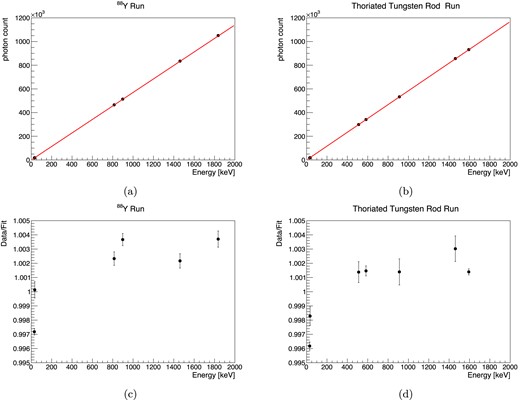
Relation between the photon counts and the corresponding energies. The lines are the fit results as proportional ((a) and (b)). The ratios of the data point to the fit are shown in (c) and (d).
The ratios of the data points to the fitted proportional lines are shown in Figs. 18(c) and (d). Linearity is good except that the Kα peaks are below the fitted line.
By extrapolating these results, we estimate the energy resolution at the Q value of 136Xe 0νββ, 2458 keV. Two cases are considered for the dependence on E: |$a\sqrt{E}$| and |$a\sqrt{E+bE^2}$|. The former is for a situation dominated by statistical fluctuation, and the latter is with the contribution of systematics. Figure 19 shows the results of the extrapolation to the Q value.
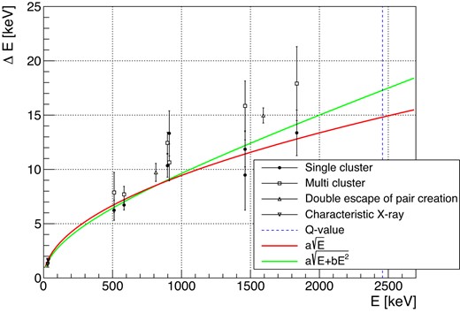
Extrapolation of the energy resolution to the Q value of 136Xe 0νββ with two kinds of fit function, |$a\sqrt{E}$| and |$a\sqrt{E+bE^2}$|. Only the single-cluster gamma-ray data points (solid circle) were used for the fit.
Note that only the data points of single-cluster gamma-ray peaks are used. The estimated energy resolution at the Q value is |$0.60 \pm 0.03\%$| for the form of |$a\sqrt{E}$| and |$0.70 \pm 0.21\%$| for the form of |$a\sqrt{E+bE^2}$|. The multiple-clustered events give slightly worse resolutions. Possible reasons for this are discussed in Sect. 5.2.5.
5.2. Breakdown of the energy resolution
Contributions from various sources to the energy resolution were evaluated for the peak of the 88Y 1836 keV gamma ray as follows.
5.2.1. Fluctuation in the signal generation process
The following five factors are considered in this category: fluctuation of the number of initial ionization electrons, recombination, attachment, fluctuation of the EL generation, and fluctuation of the MPPC non-linearity.
The fluctuation of the number of initial ionization electrons is calculated to be 0.29% with a Fano factor of 0.13 [22] and a W value of 22.1 eV [23].
The energy resolution deteriorates as the drift electric field is lowered. This is because of the recombination of ionization electrons. The energy resolution for 661.7 keV gamma rays is 0.6% at ≳100 V/cm/bar but worsens to 0.7% at the electric field at which we performed our measurement (83.3 V/cm/bar) [15]. This difference corresponds to 0.22% at 1836 keV.
The number of ionization electrons is reduced by 0.83% by attachment during the 180 mm drift with the measured attenuation length of 21 700 mm. Then, the fluctuation of this reduction is at most 0.02%.
The fluctuation of the EL generation and detection was evaluated by a simulation tuned with the measured EL gain, and was found to be 0.24%.
As discussed in Sect. 4.1.1, MPPCs suffer from non-linearity when the number of photons simultaneously incident is close to the number of pixels. This is a statistical process so the fluctuation remains even after the non-linearity is corrected. By comparing the simulations with and without this effect, the contribution was estimated to be 0.18%.
5.2.2. Calibration error
Errors in the following four corrections can contribute to the energy resolution: EL gain correction, MPPC recovery times, time variation correction, and z-dependence correction.
The contribution from the error of the EL gain correction (Sect. 4.1.2) is calculated as follows:
where ϵch is the error for each channel, |$\bar{\epsilon }$| is the mean error, |$\bar{N}_\mathrm{ch}$| is the mean photon count for each channel, |$\bar{N}$| is the mean total photon count at 1836 keV, and 2.36 is the conversion factor from the standard deviation to the FWHM. As |$\bar{\epsilon } = 0.46\%$| and |${\sum _\mathrm{ch}\bar{N}_\mathrm{ch}^2}/{\bar{N}^2} = 0.043$|, the contribution to the energy resolution is 0.23%. This result is also interpreted as |$\bar{\epsilon }/\sqrt{n_\mathrm{eff}}\times 2.36$|, where neff = 22.7 is the effective number of hit channels.
The accuracy of the MPPC recovery time measurement affects the energy resolution in two ways: the precision of an individual MPPC’s recovery times and overall bias. The recovery times of individual MPPCs were measured with about 0.5 ns precision. Its effect was estimated by simulation and found to be negligible. The effect of the overall bias is evaluated based on Eq. (1) in Sect. 4.3.5. After the overall fine-tuning of the recovery times, Δk is −0.29 ±1.84 × 10⁻⁶, consistent with zero, which is thanks to the fine-tuning. For 1836 keV events, the FWHM of the distribution of CSS is 6.15 × 10⁸, and therefore the contribution to the energy resolution is at most |$\sqrt{0.29^2+1.84^2}\times 10^{-6}\times 6.15\times 10^8/\left(1.05\times 10^6\right) = 0.11\%$|.
The time variation correction factor is determined from the Kα peak fit in each time bin (Sect. 4.3.3). The average fit error is 0.137%; therefore the error of the scale factor is also 0.137%, and the contribution to the energy resolution is 0.32%, multiplied by 2.36.
The variation within the time bin is also evaluated. There is at most 0.24% variation in a time bin of 30 minutes. Assuming that the variation in the time bin is uniform, the contribution to the energy resolution is at most |$0.24\%\times \frac{2.36}{\sqrt{12}}=0.16\%$|.
When there is an error in the attenuation length determination, the error from the z-correction (Sect. 4.3.4) on the photon counts is calculated as
where pi is the correction factor other than the z-dependence correction, zi is the z-position of each sampling of the waveform, λ′ is the attenuation length used in the correction, λ is the true attenuation length, and |$\bar{z}$| is the z-position of the event given as the mean weighted by the photon counts. Figure 20 shows the distribution of Ncor versus |$\bar{z}N_\mathrm{cor}$|.
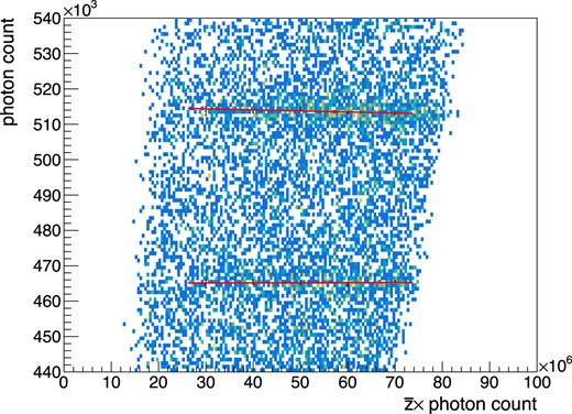
Relation between the corrected photon counts (Ncor) and the product of the photon counts and the mean z-position (|$\bar{z}N_\mathrm{cor}$|). The clusters at ∼5.1 × 10⁵ photons and ∼4.6 × 10⁵ photons correspond to the photopeak of 898 keV gamma rays and the double escape peak of 1836 keV gamma rays, respectively.
1/λ′ − 1/λ would appear as a slope of clusters. From this plot, 1/λ′ − 1/λ is obtained as −1.52 ±1.12 × 10⁻⁵ mm−1, consistent with zero. Because the FWHM of the distribution of |$\bar{z}N_\mathrm{cor}$| for 1836 keV events is 6.03 × 107 mm, the contribution to the energy resolution is at most |$\sqrt{1.52^2+1.12^2}\times {10}^{-5}\times 6.03\times {10}^{7}$| photons, i.e., 0.11%.
5.2.3. Hardware-origin error
Position dependence of the EL gain and errors arising from the waveform processing in the FEB are considered.
The EL gains depend on the injection positions of ionization electrons relative to the cell. The amount of the dependence was estimated from the calculated electric field distribution [13] and the effect on the energy resolution was found to be negligible by comparing the results of simulations with and without this dependence.
In the FEBs, the signal waveforms are shaped by Sallen–Key filters and then digitized. The effect of this filtering and digitization was evaluated by simulation and was found to be negligible.
The baseline of the waveform is unknown within one ADC count. This leads to two effects on the energy reconstruction. First, event-by-event fluctuation of the unknown offset causes fluctuation in the photon count determination. In addition, since the event time width itself fluctuates, the offset affects the photon count determination even if it is constant. The contribution to the energy resolution from the baseline offset is calculated from the mean and standard deviation of the event time width and was found to be 0.09% at most. The contributions from hardware are small. This is natural because they were so designed.
5.2.4. Mis-reconstruction of z-position
If the primary scintillation is wrongly identified, the z-position of the event is mis-reconstructed and the correction of z-dependence is wrongly applied. Figure 21 shows the distribution of the number of hit clusters for the primary scintillation light candidates for 1836 keV events.
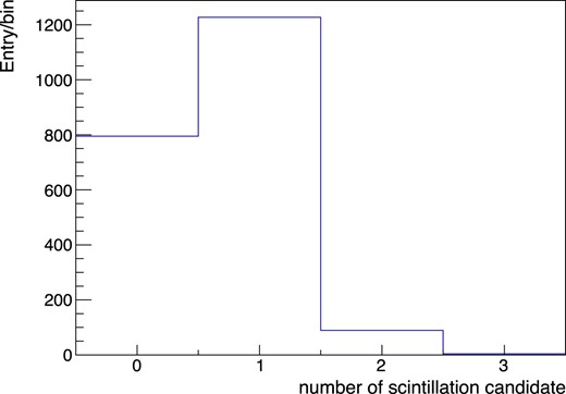
Number of candidates for the primary scintillation light for 1836 keV events.
Assuming that the efficiency of detecting the right scintillation light is ε and the average number of detected accidental scintillation hits is μacc, the probabilities that no or just one hit cluster is detected as a primary scintillation light candidate are as follows:
From Fig. 21, it follows that ε = 0.60 and μacc = 0.075. Since only the events with just one hit cluster are chosen in the analysis, the probability of mis-reconstruction of the z-position is |$\frac{\left(1-\varepsilon \right)\mu _\mathrm{acc}e^{-\mu _\mathrm{acc}}}{P\left(n_\mathrm{sci}=1\right)}=5\%$|. Assuming that the mis-reconstruction distributes uniformly from 0 to 180 mm, the mis-correction of z-dependence uniformly distributes from 0 to 0.83%. Then, the contribution to the energy resolution is |$\sqrt{5\%}\times \frac{0.83\%}{\sqrt{12}}\times 2.36=0.13\%$|.
5.2.5. Summary of the energy resolution breakdown and prospect of improvement
Table 2 summarizes the breakdown of the energy resolution at 1836 keV.
Breakdown of the energy resolution at 1836 keV listed in descending order.
| Error in the time variation correction | 0.32% |
| Fluctuation of the number of initial ionization electrons | 0.29% |
| Fluctuation of the EL generation and detection | 0.24% |
| Error in the EL gain correction | 0.23% |
| Recombination | 0.22% |
| Fluctuation of the MPPC non-linearity | 0.18% |
| z mis-reconstruction | 0.13% |
| Variation in time bin of time variation correction | ≲ 0.16% |
| Error in the z-dependence correction | ≲ 0.11% |
| Accuracy of the MPPC recovery times | ≲ 0.11% |
| Offset of the baseline | ≲ 0.09% |
| Fluctuation of the attachment | ≲ 0.02% |
| Position dependence of the EL gain | 0% |
| Waveform processing in the FEB | 0% |
| Estimation total | |$0.63\% \ {\rm to}\ 0.67\%$| |
| Data total | |$0.73 \pm 0.11\%$| |
The total estimated energy resolution is 0.63–0.67% while the measured energy resolution is |$0.73 \pm 0.11\%$|. These are in agreement within the margin of error. The estimation was made for the single-clustered track case. We figure that the worse energy resolution for the multiple-clustered events is because of larger contributions from recombination, fluctuation of the MPPC non-linearity, and accuracy of the MPPC recovery times.
The fluctuation of the EL generation and detection can be suppressed by increasing the detected number of photons. We are developing a new ELCC with MPPCs with sensitive areas approximately twice as large and anode electrodes with higher discharge resistance. Recombination can be suppressed by applying a stronger drift electric field, which is now limited by the discharges at the ELCC. The accuracies of the EL gain correction and the time variation correction are limited by the statistics of the Kα peak events and therefore can be reduced by taking more data with a steadier condition. Mis-reconstruction of the z-position comes from the limited efficiency of the primary scintillation detection, which is now 1 p.e. level. We are developing a wavelength-shifting-plate configuration to improve the efficiency of primary scintillation detection and reduce mis-reconstruction using the information of photon counts. With these countermeasures, the total energy resolution is expected to be improved down to 0.37% (FWHM) at 1836 keV, which corresponds to 0.32% (FWHM) at the Q value.
5.3. Track reconstruction
Figures 22 and 23 are typical reconstructed track images of a 2615 keV event and a 1593 keV event.
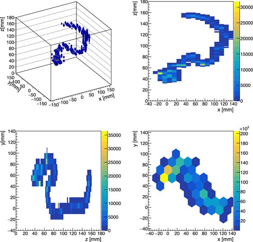
Reconstructed track image of a 2615 keV event. This is considered to be a photoabsorption event.

Reconstructed track image of a 1593 keV event. This is considered to be a double escape event of a pair creation by a 2615 keV gamma ray.
The former is consistent with photoabsorption of a 2615 keV gamma ray from 208Tl. The latter is considered to be a double escape of a 2615 keV pair creation. A dense energy deposit at the end of the track (“blob”) can be seen in Fig. 22 and as two blobs in Fig. 23. The number of blobs will be a key to distinguishing the 0νββ signals from the gamma-ray backgrounds.
In the development of the algorithm to distinguish signals from backgrounds based on track images, the properties of track images should be understood and reproduced in simulation dataset. For this purpose, we evaluated the diffusion of the tracks. The Kα clusters, whose track lengths are about 0.8 mm, much smaller than the spread by diffusion, are selected for every 1 cm interval in the z-direction and overlaid with respect to each center position to obtain averaged hit distributions. The standard deviations of the distribution in the x-, y-, and z-directions are plotted as a function of the z-position in Fig. 24.
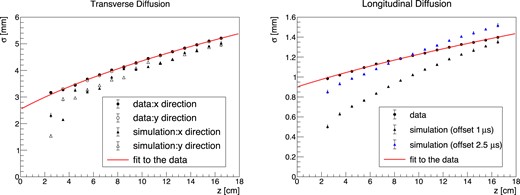
The standard deviation of the averaged hit distribution of Kα clusters in the transverse (left) and longitudinal (right) directions to the drift direction. The results for the simulation dataset are also shown.
They are fitted by the form of |$\sqrt{{p_0}^2z+{p_1}^2}$|, where the fit parameter p0 corresponds to the diffusion of ionization electrons during drift and the parameter p1 corresponds to the offset term, e.g., the pixelization at the ELCC for the transverse direction, and the low-pass filter in AxFEB and finite time of EL photon generation in the ELCC cells for the longitudinal direction. The fit results are |$p_0 = (0.1120 \pm 0.0004)\, {\rm cm}/\sqrt{{\rm cm}}$| for the transverse direction and |$p_0 = (0.0264 \pm 0.0002)\, {\rm cm}/\sqrt{{\rm cm}}$| for the longitudinal direction. The expectations calculated by Magboltz [24] are |$0.115\, {\rm cm}/\sqrt{{\rm cm}}$| for the transverse diffusion and |$0.0323\,{\rm cm}/\sqrt{{\rm cm}}$| for the longitudinal diffusion. The same analysis was performed on the simulation dataset generated with these expected diffusion constants. The simulation takes into account the generation of photons in the ELCC (|$1 \,\mathrm{\mu s}$|) and the response of AxFEB. As shown in Fig. 24, the transverse diffusion is roughly reproduced but the longitudinal diffusion differs both for the offset and z-dependence. For the longitudinal direction, an additional offset of |$1.5 \,\mathrm{\mu s}$| is added to the simulation and is also displayed in Fig. 24. The agreement between the measurement and simulation becomes better. There is, however, still disagreement, indicating that the diffusion constant is different. The diffusion constant is sensitive to the impurities in the gas, and this may be the reason for the disagreement. The simulation can be tuned using these data; this is quite important to validate the algorithms separating the 0νββ signal from the gamma-ray background based on the track image.
6. Conclusion
We have upgraded the AXEL prototype detector with a 180 L pressure vessel and evaluated the performance around the Q value of 136Xe 0νββ, 2458 keV. The number of ELCC units was increased to 12. The structure of the ELCC was also upgraded to suppress discharges. Data were taken at 7.6 bar with irradiation of 1836 keV gamma rays from an 88Y source and with thorium series gamma rays including 2615 keV from 208Tl. The obtained FWHM energy resolution is |$0.73 \pm 0.11\%$| at 1836 keV. The FWHM energy resolution at the Q value is estimated to be |$0.60 \pm 0.03\%$| when extrapolated by |$a\sqrt{E}$|, and |$0.70 \pm 0.21\%$| when extrapolated by |$a\sqrt{E+bE^2}$|. This result proves the scalability of the AXEL detector with the ELCC while maintaining a high energy resolution. The factors that determine the energy resolution were evaluated, and it was shown that further development of the ELCC will improve the energy resolution. In the reconstructed track images, the blob structures are confirmed; these correspond to the number of electrons in the event. The diffusion constants are derived from the data; this is important to develop algorithms to discriminate the signal and background based on simulated track images.
Acknowledgement
This work was supported by JSPS KAKENHI Grant Numbers 18H05540, 18J00365, 18J20453, 19K14738, 20H00159, 20H05251. We also appreciate the support for our project by the Institute for Cosmic Ray Research, the University of Tokyo. The development of the front-end board AxFEB is supported by Open-It (Open Source Consortium of Instrumentation).
References
Author notes
Present address: Institute for Advanced Synchrotron Light Source, National Institute for Quantum Science and Technology, Sendai 980-8579, Japan
