


Abstract
We investigate whether the soft mode that becomes massless at the QCD critical point (CP) causes an enhancement of the dilepton production rate (DPR) and electric conductivity around the CP through modification of the photon self-energy using the two-flavor Nambu–Jona-Lasinio model. The modification is described by the so-called Aslamazov–Larkin, Maki–Thompson, and density of states terms, which have been taken into account in our previous study on the DPR near the color-superconducting phase transition, with a replacement of the diquark modes with the soft mode of the QCD CP. We show that the coupling of photons with the soft modes brings about an enhancement of the DPR in the low-invariant-mass region and the conductivity near the CP, which would be observable in relativistic heavy-ion collisions.
1. Introduction
Exploring high-density matter at vanishing and finite temperatures in quantum chromodynamics (QCD) is one of the most challenging as well as intriguing subjects in current nuclear physics [1]. Among various interesting subjects, the possible existence of a critical point called the QCD CP on the QCD phase diagram has been receiving much attention. The phase transition at the QCD CP is of second order in the same universality class as the Z2 Ising model, and large fluctuations of various quantities coupled to the order parameter are expected to occur [2,3]. A number of proposals have been made for observational identification of the QCD CP in relativistic heavy-ion collision (HIC) experiments [1–8], such as event-by-event fluctuations of conserved charges and especially their non-Gaussianity, large fluctuations of the low-momentum particle distributions, anomalous fluid dynamical phenomena with diverging transport coefficients, and so on. Active experimental analyses are ongoing at the beam-energy scan program at RHIC, NA61/SHINE, and HADES [9]. Future experiments at FAIR and J-PARC-HI will further pursue them [10,11].
In this article, we investigate possible signals of the QCD CP that would be observed in these experiments on the basis of the fact that the second-order nature of the QCD CP implies the existence of a low-energy mode with a vanishing mass at the CP. Such a slow mode is called the soft mode of the phase transition. The soft mode of the QCD CP is represented by fluctuations in the scalar channel but it is not a sigma mesonic mode. Instead, it is a particle–hole (p–h) collective excitation with the mixing of baryon number density and energy density that has spectral support in the space-like region [12–15].
The existence of the soft mode should affect various observables near the CP. In this article, as examples of such observables, we explore how the dilepton production rate (DPR) and the electric conductivity are affected by the soft mode of the QCD CP. We have shown in a previous work [16] that the DPR can be greatly enhanced in the low-invariant-mass region near the phase boundary of two-flavor color superconductivity (2SC) due to the diquark soft mode [17–20]; in Ref. [16], the enhancement of the DPR originates from a modification of the photon self-energy by the Aslamazov–Larkin (AL) [21], Maki–Thompson [22,23], and density of states (DOS) terms [24] incorporating the diquark soft modes. A surprise in Ref. [16] was that, although the spectral support of the diquark soft mode is concentrated in the space-like region, the scattering process described by the AL term causes enhancement of the DPR in the time-like region. We thus expect that such an enhancement of these observables may occur by a similar mechanism due to the soft mode associated with the QCD CP; we consider the AL, MT, and DOS terms with the diquark soft modes being replaced by the soft mode of the QCD CP in the two-flavor Nambu–Jona-Lasinio (NJL) model.
A notable feature of the soft mode of the QCD CP is that its propagator is not analytic at the origin, unlike the diquark modes investigated in Ref. [16]. As a result, a simple time-dependent Ginzburg–Landau (TDGL) approximation is not applicable to describe the soft mode of the QCD CP. We thus introduce an approximation scheme that simply takes care of the specific analytic properties. The vertex functions in the AL, MT, and DOS terms are then constructed so as to be consistent with this treatment in light of the gauge invariance. In this way, our photon self-energy is constructed to satisfy the Ward–Takahashi (WT) identity.
Using the photon self-energy thus constructed, we calculate the DPR and the electric conductivity near the QCD CP. We show that the DPR in the low-invariant-mass region, as well as the electric conductivity, is greatly enhanced around the QCD CP due to the soft modes. We also address some issues that are relevant when pursuing an experimental measurement of these signals in the HIC experiments.
This paper is organized as follows. In the next section, after introducing the model and its phase diagram in the mean-field approximation, we discuss the properties of the soft mode of the QCD CP. In Sect. 3, we calculate the photon self-energy described by the AL, MT, and DOS terms. In Sect. 4, we discuss the numerical results of the DPR and electric conductivity near the QCD CP. The final section is devoted to a short summary.
2. Phase diagram and soft modes of QCD CP
To investigate the DPR and electric conductivity near the QCD CP, we adopt the following two-flavor NJL model [25]:
where ψ is the quark field and |$\vec{\tau }=(\tau _1,\tau _2, \tau _3 )$| is the Pauli matrices for the flavor SU(2)f. The current quark mass m = 5.5 MeV, the scalar coupling constant |$G_S=5.50~\rm {GeV^{-2}}$|, and the three-momentum cutoff Λ = 631 MeV are determined so as to reproduce the pion mass |$m_{\pi }=138~\rm {MeV}$| and the pion decay constant |$f_{\pi }=93~\rm {MeV}$| [25].
In Fig. 1, we show the phase diagram as a function of the temperature T and the quark chemical potential μ in the mean-field approximation with the mean field |$\langle \bar{\psi } \psi \rangle$|. The solid line shows the first-order critical line, and the circle marker denotes the QCD CP, which is located at |$(T_c,\, \mu _c)\simeq (46.757,\, 329.30)~{\rm MeV}$|.
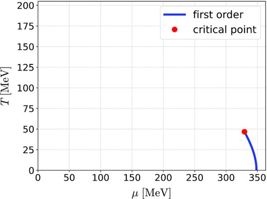
Phase diagram calculated by the mean-field approximation in the two-flavor NJL model (1). The solid line shows the first-order phase transition. The QCD CP is represented by the circle marker, which is located at (Tc, μc) ≃ (46.757, 329.30) MeV.
The soft mode of the QCD CP is described by the collective excitations of the scalar field |$\bar{\psi }\psi$| [12,26]. The imaginary-time Green’s function of this channel in the random-phase approximation (RPA) is given by [25]
where Nf = 2 and Nc = 3 are the numbers of flavor and color, |$\mathcal {Q}(k)=\mathcal {Q}(\boldsymbol {k}, i\nu _n)$| is the one-loop quark–anti-quark correlation function, |$\mathcal {G}_0(p)=\mathcal {G}_0(\boldsymbol {p}, i\omega _m) = 1/[(i\omega _m + \mu )\gamma _0 - \boldsymbol {p} \cdot \boldsymbol {\gamma } + M]$| is the free-quark propagator, ωm (νn) is the Matsubara frequency for fermions (bosons), |$M = m - 2G_S\langle \bar{\psi } \psi \rangle$| is the constituent quark mass, and Tr is the trace over the Dirac indices. Throughout this paper, we denote the momentum integration and Matsubara-frequency summation as |$\int _p = T\sum _m \int d^3\boldsymbol {p}/(2\pi )^3$|. The Green’s function |$\tilde{\Xi }(k)$| is represented by a sum of repeated bubble diagrams composed of the one-loop correlation function (3).
The retarded functions |$\Xi ^R(\boldsymbol {k}, \omega )$| and |$Q^R(\boldsymbol {k}, \omega )$| corresponding to |$\tilde{\Xi }(k)$| and |$\mathcal {Q}(k)$| are obtained by an analytic continuation iνn → ω + iη. The analytic formula of the imaginary part of |$Q^R(\boldsymbol {k}, \omega )$| is calculated to be
where |$\bar{k}(|\boldsymbol {k}|, \bar{\Lambda }) \lt |\boldsymbol {k}|$|. Then the real part is given by the Kramers–Kronig relation
where P denotes the principal value.
The first and second terms in the curly brackets in Eq. (4) take nonzero values in the time- and space-like regions, respectively. |$\Xi ^R(\boldsymbol {k},\omega )$| has poles that physically represent collective modes in the time- and space-like regions, respectively. The former corresponds to the sigma meson composed of quark–anti-quark excitations, the latter to that composed of p–h excitations due to the existence of a Fermi sphere.
From Eq. (4) one also finds that |$Q^R(\boldsymbol {k}, \omega )$| is not analytic at the origin |$(|\boldsymbol {k}|,\omega )=(0,0)$|. In fact, the limiting value of |${\rm Im} Q^R(\boldsymbol {k}, \omega )$| at the origin along the line |$\omega =a|\boldsymbol {k}|$| is given by
with |$\lambda _0 = \sqrt{4M^2/(1-a^2)}$|. Equation (8) is nonzero for |$0 \lt |a| \lt 2\Lambda /\bar{\Lambda }\lt 1$|, in which the value depends on a.
At the QCD CP, |$\Xi ^R(\boldsymbol {k}, \omega )$| satisfies
in accordance with the nature of the second-order phase transition at the CP. In fact, Eq. (9), known as the Thouless criterion [27], is derived from the stationary condition of the effective potential at the CP. The Thouless criterion shows the existence of a collective mode that becomes exactly massless1 in |$\Xi ^R(\boldsymbol {k}, \omega )$|. This mode is called the soft mode associated with the CP. It is known that the soft mode of the QCD CP is a p–h mode in the space-like region, while the mesonic mode in the time-like region does not become massless even at the QCD CP [12,14,15,26].
In the next section, we investigate the effect of the soft mode on the photon self-energy in the low-energy–momentum region. For this analysis we introduce an approximate formula of |$\Xi ^R (\boldsymbol {k}, \omega )$| that is valid near the QCD CP in the following way: First, since the spectral function of the soft mode has support in the space-like region, we focus on the strength in the space-like region only. The mesonic mode in the time-like region is neglected since its contribution to the photon self-energy at low energy–momentum is suppressed because of the dispersion relation |$\omega \gt \sqrt{\boldsymbol {k}^2+4M^2}$|, where M ≃ 185 MeV around the CP. Second, we approximate the denominator of |$\Xi ^R (\boldsymbol {k}, \omega )$| in the space-like region by expanding it with respect to ω and picking up the first two terms as
where |$A(\boldsymbol {k}) = G_S^{~-1} + Q^R (\boldsymbol {k}, 0)$| and |$C(\boldsymbol {k}) = \partial Q^R (\boldsymbol {k}, \omega )/\partial \omega \, |_{\omega =0}$|, which are found to be real and pure-imaginary numbers, respectively, from Eqs. (4) and (7). We then write the imaginary part of Eq. (10) as
where we have used the fact that |${\rm Im} \Xi ^R(\boldsymbol {k}, \omega )$| takes a nonzero value for |$|\omega |\lt \bar{k}(|\boldsymbol {k}|, \bar{\Lambda })$| in the space-like region, as seen from Eq. (4). In the next section, we use the forms of |$A(\boldsymbol {k})$| and |$C(\boldsymbol {k})$| determined in the NJL model for given T and μ. It is shown that |$C(\boldsymbol {k})$| behaves as |$1/|\boldsymbol {k}|$| and diverges in the limit |$|\boldsymbol {k}|\rightarrow 0$| corresponding to the non-analytic nature of |$\Xi ^R(\boldsymbol {k}, \omega )$| at the origin. From this behavior a simple time-dependent Ginzburg–Landau (TDGL) approximation [24] that expands |$[\Xi ^R(\boldsymbol {k}, \omega )]^{-1}$| with respect to ω and |$|\boldsymbol {k}|$| is not applicable in the present case. Our approximation (11) is valid even in this case since the |$\boldsymbol {k}$| dependence is treated exactly. We also note that the combination |$C(\boldsymbol {k})\omega \sim \omega /|\boldsymbol {k}|$| does not diverge in the |$|\boldsymbol {k}| \rightarrow 0$| limit, because of the condition |$|\omega |\lt |\boldsymbol {k}|$|.
To demonstrate the validity of Eq. (11), we show in Fig. 2 the contour maps of the dynamical structure factor given by
in the space-like region at and slightly away from the CP (T = 0.9Tc, 1.0Tc, and 1.1Tc at μ = μc). In each panel, the left and right subpanels are the results of the RPA, Eq. (2) with Eq. (4), and the approximation (11), respectively. In Fig. 3, we also show the ω dependence of |$S(\boldsymbol {k}, \omega )$| with and without the approximation (11) for several values of |$|\boldsymbol {k}|$|. One finds that |$S(\boldsymbol {k}, \omega )$| with Eq. (11) well reproduces |$S(\boldsymbol {k}, \omega )$| in the RPA, especially in the low-energy–momentum region (|ω| ≲ 50 MeV and |$|\boldsymbol {k}| \lesssim 200~{\rm MeV}$|).
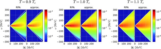
Color maps of the dynamical structure factor |$S(\boldsymbol {k}, \omega )$| in the space-like region for T = 0.9Tc, 1.0Tc, and 1.1Tc, respectively. The solid (white) lines represent the light cone. The left subpanel for each T is the result computed by the RPA (2), (3), while the right one shows the approximate formula (11).

Although the spectral properties of the soft mode of the QCD CP look quite similar to those of the diquark soft mode [16], the present |$\Xi ^R(\boldsymbol {k},\omega )$| is not analytic at the origin |$(|\boldsymbol {k}|,\omega )=(0,0)$| and it has a discontinuity at the light cone, in contrast to that of the diquark mode; the discontinuity of the diquark propagator coming from the light cone is located at |$|\omega +2\mu |=|\boldsymbol {k}|$|, and, accordingly, is analytic at the origin [16,20]. The following analysis will be done with some extra caution around this difference.
3. Dilepton production rate and electric conductivity
In this section, we shall calculate the dilepton production rate (DPR) and the electric conductivity assuming that the system is in the vicinity of the QCD CP. In this case, these observables would be significantly modified by the soft modes. Their effects can be incorporated by taking into account the soft mode fluctuations appropriately in the photon self-energy calculation. We perform this analysis in a parallel way to the analysis in Ref. [16] that investigated the diquark soft modes. Once the retarded photon self-energy |$\Pi ^{R \mu \nu } (\boldsymbol {k}, \omega )$| is obtained, the DPR is calculated to be
with the fine structure constant α and the Minkowski metric gμν. The electric conductivity σ is also obtained as [28]
3.1. Modification of photon self-energy by the soft mode
To construct the photon self-energy in a gauge-invariant way, we start with the lowest-order contribution of the soft mode to the thermodynamic potential |$\Omega _{\rm fluc} = \int _p \ln [G_S \tilde{\Xi }^{-1}(p)]$|, which is diagrammatically represented by the one-loop graph of the soft mode propagator. The photon self-energy is then constructed by attaching electromagnetic vertices at two points of quark lines in Ωfluc. This procedure leads to the 10 types of diagrams shown in Fig. 4. By borrowing the nomenclature of the theory of superconductivity [16,21,22], we call (a)–(d) the Aslamazov–Larkin (AL) [21], (e) and (f) the Maki–Thompson (MT) [22], and (g)–(j) the density of states (DOS) terms, respectively. The respective contributions to the photon self-energy, |$\tilde{\Pi }^{\mu \nu }_{\rm AL} (k)$|, |$\tilde{\Pi }^{\mu \nu }_{\rm MT} (k)$|, and |$\tilde{\Pi }^{\mu \nu }_{\rm DOS} (k)$|, in the imaginary-time formalism are expressed as
where f = u, d is the index of flavors and the vertex functions |$\tilde{\Gamma }^\mu _f(q, q+k)$|, |$\mathcal {R}_{{\rm MT},f}^{\mu \nu }(q, k)$|, and |$\mathcal {R}_{{\rm DOS},f}^{\mu \nu }(q, k)$| are graphically represented by the three- and four-point diagrams in Fig. 4, respectively. We note that the number of diagrams is doubled compared with the case in Ref. [16], since the quark and anti-quark lines should be distinguished for the present case.
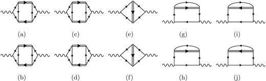
Diagramatic representations of the Aslamazov-Larkin (a)-(d), Maki-Thompson (e, f) and density of states (g)-(j) terms with the soft modes. The single, double and wavy lines are quarks, soft modes and photons, respectively.
The total photon self-energy reads
where |$\tilde{\Pi }_{\rm fluc}^{\mu \nu } (k)$| is the contribution from the soft modes and
is the self-energy of the free-quark system, where |$C_{\rm em} = e_u^2+e_d^2$| with eu = 2|e|/3 (ed = −|e|/3) denoting the electric charge of the up (down) quark. We note that |$\tilde{\Pi }^{\mu \nu } (k)$| thus constructed nicely satisfies the Ward–Takahashi (WT) identity
3.2. Vertices
For the vertex functions |$\tilde{\Gamma }^\mu _f(q, q+k)$|, |$\mathcal {R}_{{\rm MT},f}^{\mu \nu }(q, k)$|, and |$\mathcal {R}_{{\rm DOS},f}^{\mu \nu }(q, k)$|, instead of calculating the diagrams in Fig. 4 directly, we determine their functional forms from the WT identities for the vertices:
where |$\mathcal {R}^{\mu \nu }(q, k)= \mathcal {R}_{{\rm MT},f}^{\mu \nu }(q, k)+\mathcal {R}_{{\rm DOS},f}^{\mu \nu }(q, k)$|.
Among the vertex functions, only their spatial components are needed for the calculations of Eqs. (13) and (14), because |$\tilde{\Pi }_{\rm fluc}^{00}(k)$| in Eq. (13) is obtained from the spatial components through
To obtain |$\tilde{\Gamma }^i_f (q, q+k)$| for i = 1, 2, 3, we take the same procedure as that adopted in Ref. [16], where the energy-dependent and independent terms of |$\tilde{\Xi }^{-1}(q)$| on the right-hand side in Eq. (22) are attributed to |$k_0\tilde{\Gamma }^0_f (q, q+k)$| and |$\boldsymbol {k}\cdot \tilde{\boldsymbol \Gamma }_f (q, q+k)$| on the left-hand side, respectively, so that the spatial part of Eq. (22) is given by2
We then employ an ansatz in the form of |$\tilde{\Gamma }^i_f (q, q+k)$| that satisfies Eq. (25) as
Since |$A(\boldsymbol {q})$| is real, |$\tilde{\Gamma }^i_f (q, q+k)$| is also a real function in this construction. We note that this form of approximation is valid only for sufficiently small k, as the WT identity (22) cannot uniquely determine the vertex in general. However, near the QCD CP at which the contribution of the soft mode becomes prominent, it is expected that the qualitative result does not depend on the form of the vertex and our approximation would be well justified.
The form of the vertex |$\mathcal {R}_{f}^{ij}(q, k)$| is also obtained by adopting a similar argument with Eqs. (23) and (26), as was done in Ref. [16]. Even though we do not go into the details here, it can be shown that |$\mathcal {R}_{f}^{ij}(q, k)$| constructed with Eq. (26) is a real function independent of iνl and satisfies the WT identity (23). By constructing the MT and DOS terms from the vertex, one finds
Equation (28) is shown from the fact that the sum of Eqs. (16) and (17) becomes real after the Matsubara summations as long as the approximated |$\mathcal {R}_{f}^{ij}(q, k)$| is a real function independent of iνl [16,29]. The cancellation of the MT and DOS terms is also known in metallic superconductivity [24].
From Eqs. (28) and (24), one obtains
Plugging this into Eq. (13), one finds that the DPR is written solely in terms of the AL term. This is also the case for the electric conductivity since it is given by the spatial components of |${\rm Im}\Pi _{\rm fluc}^{R\mu \nu }(\boldsymbol {k},\omega )$| as in Eq. (14). These results show that we only have to compute the AL term to obtain both the DPR and the electric conductivity.
3.3. Aslamazov–Larkin term
Since |${\rm Im}\tilde{\Pi }_{\rm fluc}^{ij}(k)$| consists of only the AL term, we now calculate |$\tilde{\Pi }_{\rm AL}^{ij}(k)$|. Using Eqs. (11) and (26), we obtain
where the contour C encircles the imaginary axis. The analytic continuation of |$\tilde{\Xi } (q)$| has a cut on the real axis. From this structure, the integrand of the dq0 integral in Eq. (30), |$\tilde{\Xi } (q+k) \tilde{\Xi } (q)$|, has cuts at Req0 = 0 and −iνl. By deforming the contour C, avoiding these cuts, the q0 integral is transformed into integrals of real variables [24].
Taking the analytic continuation iνl → ω + iη after the deformation of the contour C and using Eq. (29), we obtain
The contribution of the soft mode to the DPR is computed by substituting Eq. (31) into Eq. (13). The contribution of the soft mode to the electric conductivity is also obtained by plugging the formula
into Eq. (14). We note that Eq. (32) at |$|\boldsymbol {k}|=0$| is linearly dependent on ω in the ω → 0 limit, and hence the conductivity σ calculated from it has a nonzero value. This term leads to the divergence of σ at the QCD CP, as we will see in the next section.
We note that the domain of the integral in Eqs. (31) or (32) is subject to a constraint that Eq. (11) takes a nonzero value only in the energy–momentum region |$|\omega |\lt \bar{k} (|\boldsymbol {k}|, \bar{\Lambda })$|, i.e., inside the space-like region. Nevertheless, we note that some multiple soft mode processes can affect the photon self-energy in the time-like region that is responsible for the DPR and conductivity. These contributions are understood as the scattering process of the photon with a soft mode: Let a virtual photon with the energy–momentum |$k=(\boldsymbol {k}, \omega )$| be absorbed by a soft mode with |$q_1=(\boldsymbol {q}_1, \omega _1)$| to make another one with |$q_2=(\boldsymbol {q}_2, \omega _2)$|, both of which are in the space-like region: |$|\omega _1|\lt |\boldsymbol {q}_1|$| and |$|\omega _2|\lt |\boldsymbol {q}_2|$|. Then, the energy–momentum conservation law tells us that |$\boldsymbol {k}=\boldsymbol {q}_2-\boldsymbol {q}_1$| and ω = ω2 − ω1, where |$|\boldsymbol {k}|$| can be taken arbitrarily small while keeping ω = ω2 − ω1 finite. Thus, the soft mode that has spectral support in the space-like region can contribute to the photon self-energy in the time-like region (|$\omega \gt |\boldsymbol {k}|$|). In the next section we shall see that this can cause an enhancement of the DPR and conductivity.
Before closing this section, let us clarify the limitations of our calculation. Firstly, in our treatment we focus on the effects of the soft mode in the space-like region, and the effects of the mesonic mode in the time-like region are neglected. This approximation is justified as long as we consider the DPR in the low-energy region near the QCD CP, since the mass of the sigma mode is larger than 2M ≃ 370 MeV. When considering the DPR above 2M, however, the effect of the mesonic modes will become significant. Secondly, we have constructed approximate forms of the vertex functions through the WT identities and Eq. (10). While this assumption should be valid for sufficiently small ω, it would not be directly applicable to the large energy–momentum region.
4. Numerical results
In this section, we shall show the numerical results of the DPR (13) and electric conductivity (14) near the QCD CP calculated with the photon self-energy obtained in the previous section.
We first show the DPR at |$\boldsymbol {k}=\boldsymbol {0}$| at μ = μc for several values of T below (above) Tc in the left (right) panel of Fig. 5. The thick red lines show the contribution from |$\tilde{\Pi }^{\mu \nu }_{\rm fluc} (k)$|. The total rate is given by the sum of the contributions from |$\tilde{\Pi }^{\mu \nu }_{\rm fluc} (k)$| and |$\tilde{\Pi }^{\mu \nu }_{\rm free} (k)$|. However, the latter contribution vanishes for |ω| < 2M, where M ≃ 185 MeV at the QCD CP, and it is not shown in the figure. For comparison, the DPR from the massless free-quark gas is shown by the thin blue lines in the figure. The figure shows that the DPR is enhanced significantly near the QCD CP by the soft modes and well exceeds the case of the massless free-quark gas in the low-energy region ω ≲ 250 MeV. The enhancement in the low-energy region becomes more prominent as T approaches Tc from both sides of the temperature. Taking a closer look at these results, one finds that the DPR increases monotonically as T approaches Tc from below in the left panel, while the T dependence for T > Tc shown in the right panel is not monotonous. The latter can be accounted for as a competition between the softening of the soft mode near Tc and the increase of the thermal effects at higher T. Figure 6 shows the numerical results of the DPR at nonzero momentum for several T above Tc. One finds that the enhancement of the DPR is more prominent in the lower-momentum region.
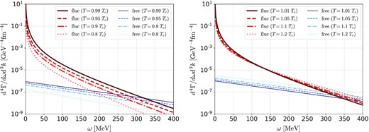
Dilepton production rate (DPR) per unit energy and momentum d 4Γ/dωd 3k for several values of T/Tc at μ = μc and |$\boldsymbol {k}=\boldsymbol {0}$|. The thick (red) and thin (blue) lines are the contributions from the soft mode and the massless quark gases, respectively. The left and right panels show the DPR below and above Tc, respectively.
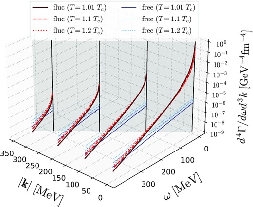
DPR d 4Γ/dωd 3k with the finite momentum |$\boldsymbol {k}$| for T/Tc = 1.01, 1.1, and 1.2 at μ = μc. The gray surface shows the light cone.
In the HIC experiments, the DPR is usually observed as a function of the invariant mass mll,
to remove the effect of the flow. In Fig. 7, we show the numerical results of Eq. (33) for various values of T at μ = μc. We find that the contribution of the soft modes is conspicuous in the low-invariant-mass region mll ≲ 150 MeV.
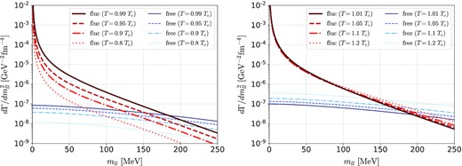
Invariant-mass spectrum |$d\Gamma / dm_{ll}^2$| at μ = μc. Left: For T/Tc = 0.8, 0.9, 0.95, and 0.99. Right: For T/Tc = 1.01, 1.05, 1.1, and 1.20.
Finally, we show the behavior of the electric conductivity σ near the QCD CP in Fig. 8. The left panel shows the T dependence of σ at three values of μ, where σ is normalized by TCem. As expected from the infrared behavior of the soft modes in the critical region, the conductivity σ tends to diverge near the CP. In fact, it can be shown that σ grows as |T − Tc|−2/3 in the vicinity of the critical point in the present approximation, as will be discussed in detail in a forthcoming publication [29]. At μ = 0.99 μc, the conductivity is not divergent but shows a prominent peak at T ≃ 1.08 Tc in accordance with the crossover nature of the transition. At μ = 1.01 μc, σ shows a cusp-like behavior, reflecting the first-order nature of the phase transition at T ≃ 0.9 Tc. The right panel of Fig. 8 shows a contour plot of σ/TCem on the T–μ plane. One sees that σ has a significant excess along the critical lines of the first-order phase and crossover transitions.
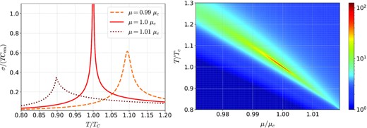
Electric conductivity σ associated with the soft modes. Left: T dependence of σ. The results of μ/μc = 0.99, 1.0, and 1.01 are shown by dashed, solid, and dotted lines, repectively. Right: Contour plot of σ in the T–μ plane around the QCD CP.
5. Discussions
Focusing on the collective soft modes, the mass of which tends to vanish at the QCD CP, we have explored their effects on the dilepton production rate (DPR) and the electric conductivity near the QCD CP. The contribution to these observables was taken into account through the modification of the photon self-energy by the AL, MT, and DOS terms, the inclusion of all of which is necessary to assure the WT identity. We have shown that the DPR in the low-energy and low-invariant-mass regions is greatly enhanced due to the soft modes around the CP, in comparison with that of the massless free-quark gas. We have also seen that a prominent enhancement of the electric conductivity σ occurs near the QCD CP due to the soft modes. We plan to report on more detailed analyses of the possible anomalous transport properties including the electric conductivity and relaxation time near the QCD CP, as well as the phase boundary of the 2SC phase, elsewhere [29].
It would be interesting to explore the phenomenological consequences of the present findings in the HIC experiments. If an anomalous enhancement of the DPR in the low-mass region, say less than 150 MeV, should ever be detected, our result suggests that it may be the signal of the QCD CP. The enhancement of the conductivity at the CP will also be observed in the HIC through a detailed analysis of the DPR in the ultra-low-energy–momentum region [30]. To identify the DPR enhancement as the QCD CP signal, however, it is important to disentangle other effects that induce a similar enhancement of the DPR. For example, in our previous study we pointed out that a similar enhancement of the DPR manifests itself near the phase boundary of the 2SC phase due to the development of diquark soft modes [29]. Other standard mechanisms due to medium effects, such as hadronic rescatterings [31] and the bremsstrahlung described by perturbative QCD [32,33], also bring about the enhancement in the low-mass region. A more detailed investigation of the invariant-mass spectrum of the DPR will be required to disentangle these effects.
Other important issues to be examined are the effects of evolution dynamics. In the dynamical evolution of the HIC, the effect of the critical slowing down will modify the DPR around the QCD CP. To deal with this effect, an analysis of the DPR in the real-time formalism with a time-dependent background medium is required. It will also be important to understand the effects of phase transitions on the bulk evolution of the medium [34]. To elucidate the production mechanisms and the respective characteristics, one would eventually need recourse to some dynamical transport models [35–38]. These investigations are left for future study. Nevertheless, we would like to emphasize that the production mechanism of the DPR through the soft modes is robust.
The measurements of the DPR in the low-invariant-mass region mll ≲ 100–200 MeV is also a challenge on the experimental side, because di-electrons are contaminated by Dalitz decay in this energy region. In spite of these challenging demands, however, it is encouraging that the future HIC programs in GSI and J-PARC-HI are designed to carry out high-statistical experiments [9–11], and also that new technical developments are vigorously being made [30].
Finally, we remark that a complete description of the collective soft modes around the QCD CP needs to incorporate the vector coupling [39,40] as well as the scalar couplings, which was exclusively taken into account in the present study. Such a more complete analysis constitutes one of the future tasks, which we hope to report sometime in the future.
Acknowledgement
The authors thank Berndt Mueller, Hirotsugu Fujii, and Akira Ohnishi for valuable comments. T.N. thanks JST SPRING (Grant No. JPMJSP2138) and the Multidisciplinary PhD Program for Pioneering Quantum Beam Application. This work was supported by JSPS KAKENHI (Grants No. JP19K03872, No. JP19H05598, No. 20H01903, No. 22K03619).
Funding
Open Access funding: SCOAP3.
Footnotes
The term “massless” here means that the pole of |$\Xi ^R(\boldsymbol {k}, \omega )$| gets to exist at the origin |$(|\boldsymbol {k}|, \omega ) = (0, 0)$| at the QCD CP: Indeed the pole of |$\Xi ^R(\boldsymbol {k}= \boldsymbol {0}, \omega )$| moves continuously toward the origin in the complex energy plane as T and μ approach the CP.
