


Abstract
Degree correlation plays a crucial role in studying network structures; however, its varied forms pose challenges to understanding its impact on network dynamics. In this study, a method is devised that uses eigenvalue decomposition to characterize degree correlations. Additionally, the applicability of this method is demonstrated by approximating the basic and type reproduction numbers in an epidemic network model. The findings elucidate the interplay between degree correlations and epidemic behavior, thus contributing to a deeper understanding of social networks and their dynamics.
Network science provides a powerful tool for understanding complex systems, in which entities are represented as interconnected nodes and their relationships as links [1–5]. This tool has aided the elucidation of the structure and dynamics of various systems, such as social networks, biological interactions, and the Internet. The study of network structures, such as degree distributions, degree correlations, and clustering, has revealed universal principles with interdisciplinary applicability. By leveraging insights from network science, real-world systems can be better understood and effective strategies and interventions can be developed.
This study focuses on degree correlation, which refers to the relationship between the degrees of connected nodes in a network. The degree of a node represents the number of connections that it contains, and the degree correlation indicates whether nodes with similar degrees tend to be connected (positive correlation or assortativity) or nodes with different degrees tend to be connected (negative correlation or disassortativity). However, degree correlations are complex and cannot be divided based on whether they are positive or negative. In particular, when the degree distribution has a fat tail, restrictions on the links between hubs cause structural disassortativity [4,6]. Therefore, the effect of the degree correlation on the spread of infectious diseases is not necessarily simple and remains unclear.
The characteristics of degree correlation are herein expressed using eigenvalue decomposition. Some studies have performed eigenvalue decomposition of adjacency matrices [7,8]. However, to the best of the author’s knowledge, no prior study has focused on eigenvalue decomposition for matrices that represent degree correlation, which is explored in this study. We apply this method to social networks and derive approximate expressions for the basic and type reproduction numbers for an epidemic network model.
The degree distribution pk is defined as the probability that a randomly selected node has degree k. The probability distribution of the degree at one end of a randomly selected link is called the excess degree and is given by
where 〈k〉 = ∑kkpk. It must be noted that pk and qk constitute kmax-dimensional vectors if the maximum degree is kmax and isolated nodes (with degree zero) are excluded. Let ehk be the probability that the two ends of a randomly selected link are nodes of degrees h and k [4,5]. If each degree is independent,
The eigenvalue decomposition of matrix ehk − qhqk yields the following equation:
where λi is the eigenvalue of the symmetric matrix ehk − qhqk on the order |λ1| ≥ |λ2| ≥ |λ3|⋅⋅⋅ and f(i) are the corresponding eigenvectors. The summation in Eq. (3) over the rank of matrix ehk − qhqk yields the exact expression, whereas stopping the summation at the appropriate point yields an approximate formula.
The degree correlation is described using the Pearson correlation coefficient between the degrees at the two ends of the same link:
This coefficient is also referred to as the assortativity coefficient [9]. By substituting Eq. (3), the following result is obtained:
where the following notation is used:
Thus, if |λ1| ≫ |λ2|, the positivity or negativity of λ1 determines the positivity or negativity of r. To characterize the degree correlation in more detail, the average degree of the nearest neighbors knn(k) is used [10]. Using Eq. (3), it can be calculated as
The eigenvalue decomposition (as aforementioned) was adopted in the eight empirical social networks and two artificial networks shown in Table 1. Figure 1(a) shows the eigenvalues up to the sixth order of the absolute value (the first and second eigenvalues are shown in Table 1). The first eigenvalue is prominent for networks MPC, CoE, and EmE (and to a lesser extent in TaW), which have strong, negative-degree correlations and small clustering coefficients. However, in the cases of EmD, CoM, and CoC, the first and second eigenvalues have almost absolute values, thus suggesting that the first eigencomponent alone cannot describe the degree correlation. Figure 1(b) shows the behavior of the degree correlation coefficient r when the eigenvalue expansion is approximated to the ith order (1 ≤ i ≤ 6), and Table 1 lists the difference between the approximation for i = 6 and the actual value of r. Again, in networks MPC, CoE, EmE, and TaW, the negative correlation is better reproduced with fewer components than in the other networks. On the other hand, for the artificial networks ADN and AAN, convergence is relatively slower than for the real networks, but for i = 6, they have rather good approximations. Figure 2 presents a comparison of knn(k) when only the first eigencomponent is considered with the actual knn(k) (the former is shown in blue, the latter in red), and the number d in each panel is the relative deviation, which is the average of the absolute values of the deviations divided by the average excess degree 〈k2〉/〈k〉. In the cases of MPC, CoE, EmE, TaW, and FrB, the approximation reproduces the tendency of the degree correlation well, whereas in the cases of CoM, ADN, and AAN, the discrepancy is significantly large. For EmD, it can be said that the trend of degree correlation, which is neither positive nor negative, is qualitatively reproduced.
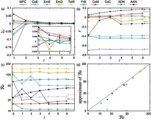
Eigenvalue decomposition results for the eight real and two artificial networks shown in Table 1. (a) Eigenvalues of the matrix ehk − qhqkz with the six largest absolute values. The inset is a magnified view. (b) Degree correlation coefficient r considered up to the ith order in the eigenvalue decomposition given by Eq. (5). The arrows on the right edge of the panel indicate the actual value of r. (c) The value of the basic reproduction number |$\mathcal {R}_{0}$| is calculated based on Eq. (16) when β = 1. The arrows on the right edge indicate the value of |$\mathcal {R}_{0}$| given by the spectral radius of Eq. (15). For i = 0, there is no degree correlation and |$\mathcal {R}_{0}=\langle k^2\rangle /\langle k\rangle$|. The discrepancy between the approximate values at i = 6 and the true values indicated by the arrows is shown in the far right columns of Table 1. (d) Relationship between the actual |$\mathcal {R}_{0}$| and the |$\mathcal {R}_{0}$| given by the approximation of Eq. (17) when β = 1.
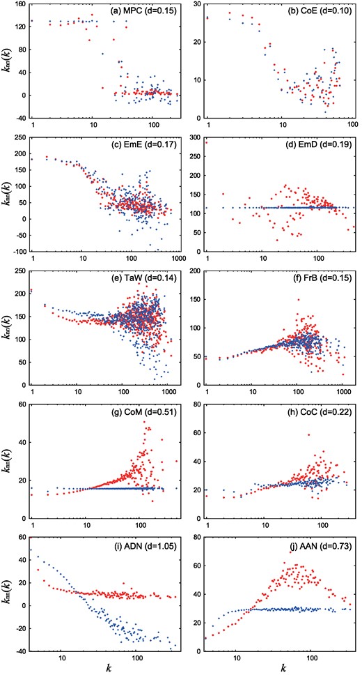
Average degrees of the nearest neighbors knn(k) (red) for the eight actual networks and the first-order approximation (blue) based on eigenvalue decomposition, as shown in Eq. (7).
Examples of real social networks and artificial networks. Eight real networks are sorted in ascending order with respect to the degree correlation coefficient r: (MPC) personal mobile phone call network among a small set of core users at the Massachusetts Institute of Technology [11,12], (CoE) coauthorship network among mathematicians who coauthored papers with Erdös (Erdös number is one) or with those mathematicians (Erdös number is two) [11,13], (EmE) network of email communications at a large European research institute [14], (EmD) network of email communications at the Democratic National Committee (DNC) [11], (TaW) communication networks on the Talk Page in Wikipedia [11,15], (FrB) friendship networks in Brightkite, which was once a location-based social networking service [16], (CoM) coauthorship network among mathematicians on the mathematical review collection of the American Mathematical Society (MathSciNet) [11,17], and (CoC) coauthorship network among physicists on arXiv cond-mat (condensed matter physics) [11,18]. Two artificial networks are constructed by using the Xulvi-Brunet–Sokolov algorithm [19]: (ADN) and (AAN) are created by rewiring the links to have disassortativity and assortativity with probability p = 0.8, respectively. Each column shows the number of nodes, number of links, average degree, maximum degree, matrix rank ehk − qhqk, degree correlation coefficient r, average clustering coefficient C, the first and second eigenvalues of the matrix ehk − qhqk, the difference between the sixth-order approximation and the actual value of r, and the ratio of the sixth-order approximation and the exact value of |$\mathcal {R}_{0}$|.
| Network | Nodes | Edges | 〈k〉 | kmax | Rank | r | C | λ1 | λ2 | r(6) − r | |$\mathcal {R}_{0}^{(6)}$|/|$\mathcal {R}_{0}$| |
|---|---|---|---|---|---|---|---|---|---|---|---|
| (MPC) Mobile phone call [11,12] | 6809 | 7680 | 2.3 | 261 | 74 | −0.68 | 0.02 | −0.1753 | 0.0036 | −0.01 | 1.01 |
| (CoE) Collaboration—Erdös [11,13] | 5094 | 7515 | 3.0 | 61 | 56 | −0.44 | 0.07 | −0.0709 | −0.0044 | 0.00 | 1.00 |
| (EmE) Email—EU [14] | 32 430 | 54 397 | 3.4 | 623 | 232 | −0.38 | 0.11 | −0.0621 | 0.0023 | −0.01 | 1.01 |
| (EmD) Email—DNC [11] | 906 | 12 085 | 26.6 | 462 | 134 | −0.09 | 0.61 | 0.0220 | 0.0139 | 0.05 | 1.02 |
| (TaW) Talk—Wikipedia [11,15] | 92 117 | 360 767 | 7.8 | 1220 | 485 | −0.03 | 0.06 | −0.0060 | 0.0006 | 0.01 | 1.01 |
| (FrB) Friendship—Brightkite [16] | 58 228 | 428 156 | 7.4 | 1134 | 261 | 0.01 | 0.17 | 0.0055 | −0.0025 | 0.02 | 1.02 |
| (CoM) Collaboration—MathSciNet [11,17] | 391 529 | 873 775 | 4.5 | 496 | 162 | 0.12 | 0.40 | 0.0158 | 0.0129 | −0.03 | 0.88 |
| (CoC) Collaboration—cond-mat [11,18] | 21 363 | 91 286 | 8.5 | 279 | 122 | 0.13 | 0.63 | 0.0077 | 0.0076 | −0.06 | 0.89 |
| (ADN) Artificial disassortative network [19] | 10 000 | 39 990 | 8.0 | 337 | 101 | −0.13 | 0.01 | −0.0366 | 0.0157 | 0.00 | 0.99 |
| (AAN) Artificial assortative network [19] | 10 000 | 39 990 | 8.0 | 337 | 101 | 0.17 | 0.01 | 0.0607 | 0.0214 | 0.01 | 0.99 |
Let us now examine the effect of degree correlations on diffusion phenomena in social networks. The following epidemic model was considered:
where ρk(t) represents the density of infected nodes within degree class k, and ph|k is the conditional probability that a node of degree k is connected to a node of degree h and is given by ph|k = ehk/qk. Herein, β is the transmission rate, and the time scale is set such that the recovery rate is unity. Equation (8) was proposed as a degree-based mean-field approximation of the epidemic models on fat-tailed networks with a few loops [20–26].
To measure the transmission potential, the basic reproduction number |$\mathcal {R}_{0}$| was used; this is the average number of secondary infections caused by a typical infection in a completely susceptible population [27,28]. When |$\mathcal {R}_{0}\gt 1$|, the infection can spread throughout the host population, whereas when |$\mathcal {R}_{0}\lt 1$|, the infection cannot spread. The value of |$\mathcal {R}_{0}$| is given by the spectral radius of the next-generation matrix G. For Eq. (8), the component Gkh of the next-generation matrix is expressed as
which is the average number of secondary cases arising from a node of degree h to nodes of degree k [29,30]. If the following vertical and horizontal vectors are represented using bras and kets:
the next-generation matrix can be written as
Because the eigenvectors G are linearly coupled and consist of |k〉 and |f(i)〉, the eigenvalue problem for G is replaced by the eigenvalue problem for the (i + 1)-dimensional matrix as follows:
Figure 1(c) shows the spectral radius of Eq. (15) for 0 ≤ i ≤ 6, when β = 1 When i is the rank of ehk, Eq. (15) is the exact expression, whereas for a small i, this is an approximate expression. The ratios between the approximate expression for i = 6 and the exact expression are shown in the rightmost column of Table 1, with large deviations downwards for CoM and CoC.
Alternatively, if |λi| ≪ 1 for i = 1, 2, …, then another approximation is possible. Neglecting the terms above the second order of λi, an approximation of the basic reproduction number is obtained as
Considering 〈k|k〉 = 〈k2〉/〈k〉, |$\langle k|f^{(i)}\rangle = \langle f^{(i)}|k\rangle = \langle k f_k^{(i)} \rangle$| and Eq. (5), Eq. (16) can be rewritten as follows:
which is consistent with that obtained previously [30,31]. Figure 1(d) presents a comparison of Eq. (17) and the exact expression using the spectral radius of Eq. (15), and it shows that Eq. (17) is a fairly good approximation except for networks MPC, CoE, and EmE, which yield strong, negative-degree correlations. In all cases, however, it is not as accurate as the approximation of Eq. (15).
Finally, a method was devised to calculate the type reproduction number |$\mathcal {T}$|, which is used to explore the effect of immunizing a target group and is defined as the average number of secondary infections within the target group [24,32,33]. If a proportion |$1-1/\mathcal {T}$| of the target population is immunized, the spread of the infection can be suppressed. Individuals with degree kt or greater are targeted. The following matrix is introduced to calculate |$\mathcal {T}$|:
where
Matrix C consists of only those components of the next-generation matrix G that infect the target population. The type reproduction number is given by the spectral radius of the following matrix:
where I denotes the identity matrix [24,32,33]. Because this eigenvalue problem can be simplified as before, the (i + 1)-dimensional matrix is considered as follows:
The spectral radius of the following matrix was calculated:
The type reproduction number |$\mathcal {T}$| is defined only when the spectral radius of G − C or G(i) − C(i) is less than one. Figure 3 shows (as an example) the effectiveness of this approximation method for two real networks.
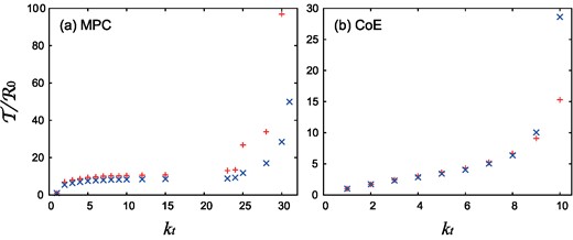
Type reproduction number |$\mathcal {T}$| (for two real networks MPC and CoE) when targeting nodes with degrees greater than or equal to kt. The red plus “+” signs represent the results obtained from Eq. (21) and the blue cross “×” signs represent the approximation from Eq. (23) with i = 1. When |$\mathcal {T}$| is finitely defined, immunizing only the target can suppress the spread of infection. This limit is independent of β, with kt ≤ 31 for MPC (kt ≤ 30 in the approximate calculation) and kt ≤ 10 for CoE (also in the approximate calculation).
In conclusion, this study has demonstrated that degree correlation can be redescribed using eigenvalue decomposition and that the next-generation matrix can be represented as a matrix of a few orders. This approximation is better for real social networks (especially disassortative ones) than for artificial networks with the Xulvi-Brunet–Sokolov algorithm [19]. This may be because this algorithm simply introduces degree correlations by rewiring the links artificially, thus not creating a gap between the eigenvalues that may exist in real social networks. This approximation method was applied to the epidemic model on networks to obtain an approximation of basic and type reproduction numbers. In addition to the approximation that cuts off the sum in Eq. (14), Eq. (17), which is an approximation when the degree correlation is small, was derived. However, the effects of loops, which cannot be ignored in networks with high-clustering coefficients, were not considered in this study. This may be why the approximation was not very good for the two assortative networks CoC and CoM with large clustering coefficients. In addition, it is necessary to introduce a correction for the difference between the SIR and SIS models, considering the infection process [34]. Finally, the proposed eigenvalue decomposition method is expected to be extensively applied to the dynamics of networks other than epidemic models.
Acknowledgement
This work was supported by JSPS KAKENHI (grant No. 21K03387). Part of this study was conducted at the Joint Usage/Research Center on Tropical Disease, Institute of Tropical Medicine, Nagasaki University (2023-Seeds-01).
