


Abstract
We compute the electron g factor to the |$\mathcal {O}(\alpha ^5)$| order on the lattice in quenched quantum electrodynamics (QED). We first study finite volume (FV) corrections in various infrared regularization methods to discuss which regularization is optimal for our purpose. We find that in QEDL the FV correction to the effective mass can have different parametric dependences depending on the size of Euclidean time t and match the ‘naive on-shell result’ only at the very large t region, t ≫ L. We adopt finite photon mass regularization to suppress FV effects exponentially and also discuss our strategy for selecting simulation parameters and the order of extrapolations to efficiently obtain the g factor. We perform lattice simulation using small lattices to test the feasibility of our calculation strategy. This study can be regarded as an intermediate step toward giving the five-loop coefficient independently of preceding studies.
1. Introduction
The anomalous magnetic moment of the electron, the electron g − 2, is one of the most precisely measured observables in particle physics. It thus gives us a good opportunity to test our understanding of quantum field theory. Theoretically the perturbative calculation of quantum electrodynamics (QED) contributions has reached the five-loop [|$\mathcal {O}(\alpha ^5)$|] level [1,2], although a slight discrepancy in the five-loop coefficient is reported [3]. The five-loop contribution is indeed relevant to the precision of the experimental measurements [4,5]. In order to examine the consistency of the Standard Model prediction with experimental results, the value of the fine structure constant is crucial, yet the value has not been determined consistently among different experiments [6].
In Ref. [7], we proposed a new method to calculate the perturbative series of the electron g − 2 using numerical stochastic perturbation theory (NSPT) [8–12]. We calculated the perturbative series to the three-loop level on small lattices. This was the first attempt to apply NSPT to QED observables. Since it can provide us with a new and alternative approach to calculating the perturbative series to high orders and can have a wide range of application, it is worth testing the usefulness of the method further.
In order to perform meaningful numerical simulations, we need to understand finite volume (FV) corrections, which are known to be severe in lattice QED because of the massless photon. In the first half of this paper, we study FV corrections in various methods of infrared (IR) regularization such as subtractions of zero modes (known as QEDL or QEDTL) and finite photon mass [13–15] to understand what kind of IR regularization is optimal, although FV corrections are not understood enough in our previous work [7]. QEDL is a famous and well-adopted regularization, and FV corrections in this regularization have been studied in many papers such as Refs. [13,14,16–20]. Mainly based on results in Ref. [14], we add a new insight into FV correction in QEDL. We find that the FV correction to the effective mass can have different parametric dependences depending on the size of Euclidean time; at 1/m ≪ t ≪ L the FV correction is given by |$\mathcal {O}(t/ ( m L^2))$|, whereas at t ≫ L it is given by |$\mathcal {O}(1/(mL))$|. The latter case matches the ‘naive on-shell result’ but this is not always true for general t. From the discussions in this part we conclude that the massive photon regularization is the most controlled method for our computation.
In the second half of this paper, we perform lattice simulation of the electron g − 2 in quenched QED, i.e. QED without the dynamical electron. We adopt finite photon mass regularization, which is found to be most suited for our purpose. In quenched QED, i.e. in sub-diagrams without lepton loops, there is a discrepancy in the five-loop perturbative coefficient between Refs. [2,21] and Ref. [3]. Our study can potentially give an independent result. As an attempt, we perform a five-loop level calculation on the lattice. Our present study does not quite give a conclusive result due to small lattice sizes. We regard the study in this paper as an intermediate step toward obtaining the continuum limit result of the five-loop coefficient.
The achievements of the present paper can be stated as follows. First, a higher-order calculation than in our previous study [7] is made possible. This is because we use a method to suppress backward propagations, which are a serious obstacle in the analysis in Ref. [7]. The higher-order calculation can be done also because numerical costs to generate configurations are drastically reduced due to quenched QED. In quenched QED, interaction terms are absent and the Langevin equation becomes trivial. Therefore, configurations are generated according to a Gaussian distribution [22–24]. In this sense, the present paper tests the efficiency of numerical calculation of perturbative series on the lattice rather than NSPT itself. Secondly, we discuss in detail the strategy for selecting simulation parameters and also the order of various extrapolations. This is based on understanding of systematic errors such as FV corrections, finite photon mass effects, which are studied in this paper.
The paper is organized as follows. In Sect. 2, we study FV corrections in various IR regularization methods to discuss what kind of IR regularization we should adopt. We also add a new insight into FV corrections in QEDL. In Sect. 3, we perform a lattice simulation. We first explain the outline of our calculation, and then we study systematic uncertainties of our calculation to discuss the strategy for selecting simulation parameters and the order of various extrapolations. Then we perform our numerical simulation following the strategy to examine its feasibility. Section 4 is devoted to the conclusions and discussion.
2. FV corrections in lattice QED
Before we attempt to calculate any physical quantities in QED, it is essential to provide a concrete definition of QED. Specially, in a FV, the treatment of IR divergence requires careful consideration to ensure that predictions agree with QED in continuum and infinite volume spacetime at a certain limit. We below discuss and compare various definitions proposed or used in the literature. We will see that the regularization by finite photon mass is the most controlled method for our g − 2 computations.
In Sect. 2.1, we study FV corrections in QEDL and QEDTL to a momentum-space correlator at one loop. This part includes already known facts and can be regarded as a review part. In Sect. 2.2, we study FV corrections in QEDL to a Euclidean time correlator, i.e. Fourier transform of the momentum-space correlator, using a result in Sect. 2.1. We point out that a FV effect has different parametric dependences depending on the size of t/L. This is the new and main result in this section. In Sect. 2.3, we consider massive photon theory and confirm exponential suppression of FV corrections for clarity.
2.1. FV corrections in QEDL and QEDTL: momentum-space correlator
We consider FV effects in various IR regularization methods: QEDL, QEDTL, and massive photon regularization [13–15]. The precise meaning of these regularizations is explained shortly.
We consider the following quantity as an example:
Here k denotes loop momentum and p external momentum. The summation/integral symbol represents the sum/integration of the loop momentum k, and its precise meaning depends on regularization schemes as discussed below. The above quantity mimics the one-loop correction to the two-point function in scalar QED. mγ denotes photon mass, which will be set to zero or nonzero below. In lattice QED, the zero mode of loop momentum k = (0, 0, 0, 0) makes the result diverge. Therefore, some regularization of the zero mode is needed. One way is to introduce nonzero photon mass. There are alternative methods which do not introduce photon mass but modify the range of loop momentum sum. QEDL and QEDTL define |$\sum\!\!\!\!\!\!\!\!\int$| as follows:
where |$\vec{k}=(k_1,k_2,k_3)$|, |$B \mathbb {Z}_{L}=\frac{2 \pi }{L} \mathbb {Z}=\lbrace \frac{2 \pi }{L} n | n \in \mathbb {Z} \rbrace$|, |$B \mathbb {Z}_{T}=\frac{2 \pi }{T} \mathbb {Z}$|, |$B \mathbb {Z}^4_{TL} =B \mathbb {Z}_{L}^3 \times B \mathbb {Z}_{T}$|, and \{0} means removal of the element (0, ⋅⋅⋅, 0). In these regularization methods, the photon mass is set to zero. We note that, although |$\mathbb {T}^3 \times \mathbb {R}$| cannot be realized in actual lattice simulations, it is convenient to consider QEDL on |$\mathbb {T}^3 \times \mathbb {R}$| as an intermediate step for clarifying the difference between QED on |$\mathbb {R}^4$| and an above theory, as explained in Ref. [17]. In other words, we can clarify FV corrections of, e.g. QEDL on |$\mathbb {T}^4$|, considering the chain (QED on |$\mathbb {R}^4$|) → (QEDL on |$\mathbb {T}^3 \times \mathbb {R}$|) → (QEDL on |$\mathbb {T}^4$|) and studying the difference of each deformation.
Eq. (1) mimics a two-point function in scalar QED and is not directly related to the g factor. Nevertheless, we understand some features of the regularization methods and obtain implications by studying this simple integral.
Below we study FV corrections in QEDL and QEDTL setting p = (0, 0, 0, p4) with |$p_4 \in \mathbb {R}$|. We note that the FV corrections to I have been studied in the case of the on-shell momentum p4 = im [14,17] and in the case of the off-shell momentum |$p_4 \in \mathbb {R}$| [14]. We give the FV corrections for the off-shell momentum also in this paper in a self-contained manner, as this result is used in the subsequent subsection. The reason why we are interested in the off-shell momentum case rather than the on-shell momentum case is that a Euclidean time correlator, which is what one actually obtains in lattice simulations, is equivalent to the Fourier integral of a momentum-space correlator I, where the integral variable p4 runs from −∞ to ∞, namely off-shell momenta. Although one might expect that this Fourier integral effectively sets p4 to the on-shell value due to the residue theorem, we point out that this understanding is too naive. This will be discussed in Sect. 2.2 after we review FV corrections to a momentum-space correlator here.
QED on |$\mathbb {R}^4$| → QEDL on |$\mathbb {T}^3 \times \mathbb {R}$|
First we consider the difference between QEDL on |$\mathbb {T}^3 \times \mathbb {R}$| and QED on |$\mathbb {R}^4$|. It is given by [13]:
Here we used the Poisson resummation to rewrite the momentum sum |$\sum _{\vec{k} \in B \mathbb {Z}_L^3 \backslash \lbrace 0\rbrace }$| by the momentum integration |$\int d^3 \vec{k}/(2 \pi )^3$| while introducing |$\vec{x} \in L \mathbb {Z}$|, where |$L \mathbb {Z}=\lbrace L n | n \in \mathbb {Z}\rbrace$|. ∫d3x corresponds to the subtraction of the spatial zero mode (since it gives |$(2 \pi )^3 \delta ^3(\vec{k})$|) and we rewrote the propagators by the Feynman parameter (y) integral and performed the momentum integration. ϑ3 denotes the elliptic theta function, |$\vartheta _3(0,e^{-\pi /s})=\sum _{n=-\infty }^{\infty } e^{-\pi n^2/s}$|.
To study the asymptotic form of ΔI for L → ∞, we consider
We can see the asymptotic behavior of ΔI by studying singularities of this function. If ΔI behaves as |$\Delta \mathrm{ I} \sim L^{-u_0}$| for L ≫ 1, |$\widetilde{\Delta \mathrm{ I}}(u)$| develops singularities at u = −u0 due to a divergence of the integral of Eq. (4) around L ∼ ∞.
We obtain
The y-integral and the s-integral are factorized. The first singularity of |$\widetilde{\Delta \mathrm{ I}}(u)$| at negative u is located at u = −2, where the y-integral diverges. This tells us that the asymptotic behavior of ΔI(L) is ΔI(L) ∼ L−2. The s-integral is convergent for u = −2. To examine the convergence of the s-integral, it is convenient to keep the following relation in mind:
where we used the Poisson resummation in the first equality and then performed the Gaussian integral. Thus, one can see that
are very suppressed functions. The expansion of |$\widetilde{\Delta \mathrm{ I}}(u)$| around u = −2 is given by
where
The inverted formula of Eq. (4) is given by
Calculating Eq. (10) by changing the integration path −i∞ → i∞ to the contour surrounding the pole at u = −2, we obtain
We note that the FV correction is singular at the on-shell momentum. This result is not new and can be understood as a special case of Eq. (46) in Ref. [14].
QEDL on |$\mathbb {T}^3 \times \mathbb {R}$|→ QEDL on |$\mathbb {T}^4$|
Next we consider the difference between QEDL on |$\mathbb {T}^3 \times \mathbb {R}$| and QEDL on |$\mathbb {T}^4$|:
In the last line, we only showed the exponential factor of the contribution which is given by the smallest possible |$|\vec{k}|$| and |x4|. (∫dk4 is performed by using the Cauchy theorem.)
QEDL on |$\mathbb {T}^4$|→ QEDTL on |$\mathbb {T}^4$|
The difference between QEDL on |$\mathbb {T}^4$| and QEDTL on |$\mathbb {T}^4$| is given by
We may give a bound |$|\Delta ^{\prime \prime } \mathrm{ I}| \le \frac{T}{L^3} \frac{1}{m^2} \sum _{n \ne 0} \frac{1}{n^2}$|. The divergence of Δ″I in the large-T limit before the large-L limit was known in Ref. [17].
The FV corrections are given by ΔI + Δ′I in QEDL on |$\mathbb {T}^4$|, and ΔI + Δ′I + Δ″I in QEDTL on |$\mathbb {T}^4$|.
We close this subsection with a remark regarding the relation between Δ′I and Δ″I. From Eq. (12), one can see that Δ′I is exponentially suppressed for 2πT/L ≫ 1. On the other hand, Δ″I is eliminated in the opposite hierarchy because of Δ″I ∼ T/L3. Therefore, if the large-L limit is taken before the large-T limit, Δ′I is not suppressed exponentially and the asymptotic behavior for L ≫ 1 needs to be clarified (although the study of the asymptotic behavior is beyond the scope of this paper). In the next subsection, we focus on QEDL and in particular its FV effect, ΔI, assuming that the large-T limit (with finite L) is taken, where Δ′I can be safely neglected.
2.2. FV corrections in QEDL: Euclidean time correlator
We consider how large FV corrections in QEDL appear in the Euclidean time correlator, which is what one can actually obtain in lattice simulations:
I∞ represents the infinite volume limit result. m2 in the numerator of the second term is added to compensate for the mass dimension. This is a rough prescription, but here we are only interested in the typical function form.
Before we insert our result Eq. (11) into the above equation, we need to consider the function form of ΔI in more detail. It is known that for the on-shell momentum p4 = im the FV correction is given by ΔI(p = im, L) ∼ 1/(mL) [14,17], which has a different L dependence from the off-shell case. In our calculation, this can be understood by setting p2 = −m2 in Eqs. (3) and (5); then the y-integral in Eq. (5) has the u = −1 singularity, which means that ΔI ∼ 1/(mL). This difference can be understood from the fact that the IR behavior of the integrand of I gets severer for the on-shell momentum than for the Euclidean momentum. From these facts, we argue that the FV correction is given by
with a constant c. This function form (15) is consistent with Eq. (11) and also with the FV correction for the on-shell momentum. We note that p2 = −m2 is not a singular point and the pole position is slightly shifted to the point |$p^2=-(1+\frac{c}{mL}) m^2$|. The constant is given by c = 4κ−3/2/κ−2 = 4 such that Eq. (15) correctly gives the FV correction for the on-shell momentum, where1
The validity of Eq. (15) in the complex p2-plane is shown in Fig. 1, where we compare Eq. (15) with numerical evaluation of Eq. (3) for Euclidean momentum p2 = 0 and momenta close to the mass shell.
![Comparison of numerical evaluation of ΔI [Eq. (3)] (black) with its asymptotic functions given by Eq. (15) (blue) and Eq. (11) (orange). They are shown as a function of 1/(mL) and p2 is chosen as p2 = 0 (left), p2 = −0.5m2 (middle), and p2 = −0.8m2 (right).](https://oup.silverchair-cdn.com/oup/backfile/Content_public/Journal/ptep/2023/10/10.1093_ptep_ptad125/3/m_ptad125fig1.jpeg?Expires=1750200193&Signature=lub4ROq-t8ZiOwHDr23I4VrKczPLtQQvG6m~O64DnYv~x5JK0Vtdl2yaY3LFT1Tbhdvy2WQZ-6c7riJ8kPO-uHMA53gCpZE-0bx3BHjXUoX-H7y0nDJSry4jsyUo4ao7guexNmZgSW1LdeKk0xiIq2uVQOCAl1CvcS~J30xyHpjPI4~7allhc2wt6BiorReOAYZ3gaS62eE7Cn5IhR1syKa5wNFJ-WDa8ljg512bgFIaap9i1AmGHgvL5PGV-aV~MlriBmsyQHwwfRRCqJPBv7pe5bY0vlgxJT-miuIHHNt3DmdWVodnMPHOqWD28P3obiU8ktrXT8cDT39PiowdqQ__&Key-Pair-Id=APKAIE5G5CRDK6RD3PGA)
Inserting Eq. (15), we obtain
In the right-hand side, the first line represents the contribution from the double pole at p4 = im and the second line the contribution from the pole at |$p_4=i m \sqrt{1+\frac{c}{m L}}$|.
We see from Eq. (17) that the FV effect for C(t) or the effective mass has different parametric dependences depending on the size of t/L. (Here, mL ≫ 1 is assumed and the time separation t is implicitly taken to satisfy mt ≫ 1 to discuss the long-distance regime.) For t/L ≫ 1, the second term of Eq. (17) is exponentially small ∼e−ct/(2L) compared with the first term and can be neglected. Then, in this case, the FV corrections to the effective mass (Meff(t) = −log [C(t)]′) are given by
The above FV correction of ∼1/L can be correctly read off from ΔI(p4 = im, L) ∼ 1/(mL), where the on-shell momentum is assumed from the beginning in calculating the momentum-space correlator.
On the other hand, for t/L ≪ 1, one can expand the exponential factor in the second term of Eq. (17) in t/L, which leads to
The 1/(mL) terms are canceled between the first and second contributions in Eq. (17). In this case the FV corrections to the effective mass are given by
The above result can also be obtained if we simply use Eq. (11). (In this case, note that p2 = −m2 is a triple pole in the integand of Eq. (14).) We note that this result cannot be obtained if one only knows ΔI(p = im, L) ∼ 1/(mL) and that the off-shell result of ΔI is essential.
For t/L ≪ 1, the FV effect is parametrically smaller than in the case of t/L ≫ 1 but gives a time-dependent effective mass as above. For t/L ≫ 1, the FV effect is larger but it is not time dependent.
The fact that the FV effect is smaller for t/L ≪ 1 may motivate one to focus on the 1/m ≪ t ≪ L region. In this case one should note that the effective mass is affected by the contribution from the branch cut starting from p2 = −m2, corresponding to the particle production cut. This drawback could be overcome by removing in advance the branch cut effect, which is calculable, from the effective mass. We calculate the branch cut effect in the Appendix in scalar QED in an infinite volume, and show that the cut effect can be largely removed from the effective mass.
We make comments on the connection with Ref. [14], where FV corrections in scalar QED have been studied in detail, and the FV effects for the pole mass of O(1/(mL)) are confirmed. In extracting the pole mass from their lattice data, a clear plateau in the effective mass has not been observed. They then have performed a subtraction of the contributions from the multiparticle states (collection of poles with 1/L intervals), after which a good plateau has been successfully obtained. They have read off the pole mass from the plateau and repeated the calculation for various L, which agrees with their expectation of the O(1/(mL)) behavior.
This conclusion is perfectly consistent with our discussion but with a little bit of complication. As discussed above, the effective mass Meff(t) is schematically expressed as the sum of the contributions from the pole at p2 = −m2 (labeled as ‘pole’) and those from the multiparticle states (labeled as ‘cut’) each with FV effects labeled as Δ, as follows:
where ⋅⋅⋅ represents the higher-order terms in the QED perturbations. The nontrivial t dependence appears from the cut contributions such as |$M_{{\rm e{}f{}f}, \infty }^{\rm cut} (t) \sim \alpha /t$|. (This behavior can be understood from the log term in Eq. (A8).) The FV effects in the cut contributions have already been discussed above and the large L behaviors are found to be that
with coefficients of O(1), c1 − 4. We also find that the FV contribution from the pole in the large volume limit is given by
where c1 is common to that in Eq. (22). This is understood from Eq. (20) where there are no O(1/L) terms for t ≪ L. In Ref. [14], the subtraction is done as |$M_{{\rm e{}f{}f}} (t) - (M_{{\rm e{}f{}f}, \infty }^{\rm cut} (t) + M_{{\rm e{}f{}f}, \Delta }^{\rm cut} (t))$|, which results in the FV effects of O(1/L) from |$M_{{\rm e{}f{}f}, \Delta }^{\rm pole}$|.
However, if we subtract only |$M_{{\rm e{}f{}f}, \infty }^{\rm cut} (t)$|, which is analytically calculable, the FV effects are obtained to be O(t/L2) by the cancellation of the O(1/L) term in the combination of |$M_{{\rm e{}f{}f}, \Delta }^{\rm pole} + M_{{\rm e{}f{}f}, \Delta }^{\rm cut} (t)$| for t ≪ L. This FV effect is parametrically smaller than O(1/L) and, in addition, the nonplateau behavior could be largely improved by subtracting |$M_{{\rm e{}f{}f}, \infty }^{\rm cut}$| alone, as indicated in the Appendix. If one applies this strategy in actual lattice computations, the FV effects may be further controlled.
We note that our study is performed with a simple and rough integrand |$\frac{1}{k^2[(k+p)^2+m^2]}$|, whereas in Ref. [14] the realistic integrand appearing in scalar QED is considered. We also note, however, that the same denominator is considered, which essentially determines the parametric dependence of FV corrections. Therefore, the simple integrand assumed in our study is sufficient to highlight the important point of our discussion. Nevertheless, it would be useful to study the FV corrections to the effective mass by starting with the realistic integrand and to give a result like Eq. (20). Then it could be possible to control FV corrections more easily. In this attempt, the technique developed in Ref. [14] might be useful.
We have observed that the FV effect in QEDL is sensitive to the IR structure (as discussed above, see Eq. (15)) and exhibits a complicated t dependence in the time correlator. In our computation aiming at obtaining the g factor to high orders, it is not realistic to correctly understand the IR structure of the relevant three-point function at each loop-expansion order and determine a proper fit function to remove FV corrections. Consequently, we find QEDL unsuited for our purpose and, therefore, consider another regularization method.
2.3. Massive photon regularization
We consider massive photon regularization with photon mass of mγL ≫ 1. In this case, the FV effects are known to be exponentially suppressed. Let us see this explicitly for clarity. I is evaluated as
The FV effect, ΔI, is given by the contributions where x ≠ 0. We obtain a bound
K0 is the Bessel function of the second kind. There exists a constant C satisfying the above inequality. In the above calculation, we assumed |$m^2 \gt m_{\gamma }^2$|, so that |$y m^2+(1-y) m_{\gamma }^2 \ge m_{\gamma }^2$|. Using the above bound, we can see that the FV effects are suppressed as |$\sim e^{-m_{\gamma } L}, e^{-m_{\gamma } T}$| by focusing on the smallest |x| contributions, which dominate ΔI.
Therefore, as long as we take mγL, mγT ≫ 1, we can safely neglect FV effects on Euclidean quantities. As can be seen from the above calculations, this is true independent of choices of the external momentum.
Since we can expect exponential suppression of FV corrections at any loop orders and any correlation functions, we will adopt finite photon mass regularization in our computation.
3. Lattice calculation of g − 2
In this section, we perform perturbative computation of the electron g factor on the lattice. We adopt photon mass regularization. In Sect. 3.1, we explain the outline of our calculation of the g factor. In Sect. 3.2, we study backward propagation and propose a method to suppress its effects. In Sect. 3.3, we study corrections to the g factor caused by finite photon mass, finite photon momentum, and a finite smearing parameter, which are introduced in our calculation (but should be finally sent to zero or infinity). In Sect. 3.4, we then discuss an optimal strategy for extracting the g factor based on our understanding of systematic errors. In Sect. 3.5, we carry out a numerical simulation following the strategy presented in Sect. 3.4.
3.1. Outline of the method
Our calculation is based on Ref. [7] to a large extent, but in order to clarify some modifications and to define quantities necessary for the discussion below, we briefly explain our calculation method here. We consider the quenched QED action on the Euclidean lattice, setting the lattice spacing a to a = 1, as
where
and |$\nabla ^2=\sum _{\mu } \nabla _{\mu } \nabla ^{*}_{\mu }$|. Here we introduce a smearing parameter ΛUV, finite photon mass mγ, and a gauge fixing parameter ξ [7]. The photon two-point function is exactly given in quenched QED as
where |$\hat{k}_{\mu } \equiv 2 \sin (k_{\mu }/2)$| and |$\hat{k}^2=\hat{k}_{\mu } \hat{k}_{\mu }$|. V denotes the four-dimensional spacetime volume. We define the Fourier transform by |$\tilde{\mathrm{ A}}_{\mu }(k)=\sum _{n} \mathrm{ A}_{\mu }(n) e^{-ik (x_n+\hat{\mu }/2)}$|. There are no quantum corrections to ξ, mγ, and the normalization of the photon wave function in quenched QED. Even though we introduce nonzero photon mass, we previously argued [7] that similar Ward–Takahashi (WT) identities to the massless photon theory hold. We can repeat a parallel argument in the quenched QED case. In particular, we can conclude that the renormalization of the coupling constant is related to the wave function renormalization of the photon as
As noted, Z3 can be exactly calculated at the tree-level due to the absence of the dynamical fermion.
We are interested in the g factor, which can be extracted from the three-point function
where the photon momentum is k, and the ingoing and outgoing fermion momenta are p and p + k, respectively. Here the matrix D is the covariant derivative acting to the fermion field in the nonquenched QED Lagrangian and given by
We denote the bare electron mass by m and the on-shell mass by mf. We define the electron propagator by
We define the vertex function Γμ(p, k) amputating the external legs,
where κ is given by a product of renormalization factors but need not be specified here. In continuum spacetime, |$\bar{u}(p) \Gamma _{\mu }(p,k) u(p+k)$| can be decomposed into two parts:
where σμν = (i/2)[γμ, γν] and the wave function satisfies |$(-i{\not{p}}-m) u(p)=0$| with |$p_0=i\sqrt{\vec{p}^2+m_f^2}$|. The g factor is defined by
To obtain the g factor on the lattice, we need to compute
and
Although the form factors are defined for the on-shell fermion, we obtain these quantities for Euclidean momenta. To read off on-shell amplitudes, we consider the Fourier transform of |$\hat{\mathrm{ G}}_{\mu }(p,k)$| and |$\hat{\mathrm{ G}}^{(\text{norm})}_{\mu }(p,k)$|. The formula we use is
where
and |$\mathcal {F}^{(\text{norm})}_E(t)$| and |$\mathcal {F}^{(\text{norm})}_M(t)$| are defined in a parallel manner by using |$\hat{\mathrm{ G}}^{(\text{norm})}$| instead of |$\hat{\mathrm{ G}}$|. The reason why we can obtain the g factor using this formula is explained in Sect. 6 in Ref. [7]. We note that systematic uncertainties, such as discretization effects and finite photon momentum effects, are left in Eq. (38) and should be removed.
We explain how to compute |$\hat{\mathrm{ G}}_{\mu }(p,k)$|. From the fact that
is invariant under the change of the integration variable Aμ(n) → Aμ(n) + ϵμ(n) (here we explicitly show that the covariant derivative (31) is a functional of Aμ), we obtain a Schwinger–Dyson equation,
Noting that the left-hand side is given by
we obtain an identity in momentum space,
In giving |$\hat{\mathrm{ G}}_{\mu }(p,k)$|, we evaluate the right-hand side, replacing δD/δAμ(ℓ) with its a → 0 limit value. The use of Eq. (44) significantly reduces the statistical error. The computation via Eq. (30) at the fixed order reduces to calculating multipoint correlation functions of photons, where the momentum conservation requires us to pick up |$\tilde{\mathrm{ A}}_\mu (k)$| in the expansion of |$\tilde{D}^{-1}$|. This is done only statistically while the above formula can skip the procedure.
We evaluate Eqs. (36) [or (44)] and (37) in perturbation theory. The perturbative formulae for δD/δAμ and D−1 are given in Sect. 2 of Ref. [7]. We note that, as explained in Ref. [7], D−1 can be evaluated fast within perturbation theory by using the fast Fourier transform. After the formal perturbative expansion of D−1 and δD/δAμ, all we have to do is to evaluate correlation functions of gauge fields, |$\langle \mathrm{ A}_{\mu _1}(n_1) \mathrm{ A}_{\mu _2}(n_2) \dots \rangle$|. Since the weight |$e^{-S[A_{\mu }]}$| is just a Gaussian, we generate configurations according to the Gaussian distribution to measure expectation values.
In our lattice calculations, we consider momenta,
with k = (0, 0, 2π/L, 0) and (2π/L, 0, 2π/L, 0). These two momenta are used for extrapolation to k2 → 0. p4 is summed over afterwards in Eq. (39) etc. For this choice, the other fermion has momenta
and the positions of the on-shell pole of S(p) and S(p + k) are the same.
3.2. Backward propagation and its suppression
The sum over p4 such as the one in Eq. (39) gives a contribution from the propagation which wraps around the torus (backward propagation). For example, let us consider
which mimics a Fourier transform of a two-point function, where E denotes energy. We obtain the exact formula for this sum,
for even t with 0 ≤ t < T and zero for odd t. z* denotes a pole in the |$z(=e^{i p_4})$|-plane and is given by |$z_*=- E+\sqrt{1+E^2}$|.
In Eq. (48), |$z_*^{T-t}$| is the backward propagation. This is an obstacle in investigating the large-t behavior because it becomes similar in size to the contribution of interest |$z_*^t$| for large t. This was actually an obstacle in our previous study [7].
Let us consider taking finer p4 in the sum,
with n = 0, 1/2, 1, 3/2, …. One can see that g(t) = f2T(t). Therefore, in this case the backward propagation is given by |$z_*^{2T -t}$| and gets milder than in the previous case.
We suppress the backward propagation in our study by taking finer p4 as in the above case. We accomplish this by changing boundary conditions for the fermion [25,26], i.e. we take the (anti)periodic boundary condition to realize (half-)integer values in the momentum summation.
3.3. Effects of mγ, k2, and |$\Lambda _{\rm UV}^2$|
The g factor obtained by Eq. (38) receives discretization effects, FV effects, and effects of modification of the Lagrangian, i.e. finite photon mass and finite |$\Lambda _{\rm UV}^2$|, and also nonzero photon momentum k2. (Although the g factor is defined for k2 → 0, we consider finite k2 in our calculation.) Here we consider effects of mγ, k2, and |$\Lambda _{\rm UV}^2$| in continuum and infinite volume spacetime because this is sufficient to evaluate their dominant effects. The FV corrections are exponentially suppressed for mγL ≫ 1 as discussed in Sect. 2.3. The discretization effects are discussed in the subsequent subsection.
Our consideration is given at the one-loop level. At one loop, it is sufficient to focus only on F2 because the one-loop contribution to F1 totally vanishes in the quantity (F1(k2) + F2(k2))/F1(k2) due to |$F_1=1+\mathcal {O}(\alpha )$| and |$F_2=\mathcal {O}(\alpha )$|. Assuming the on-shell fermion momenta |$p^2=(p+k)^2=-m_f^2$|, we have
We expressed p and k by linear combinations of |$\bar{p} \equiv (p+k)+p$| and k = (p + k) − p. They satisfy |$\bar{p} \cdot k=0$| and |$\bar{p}^2=-4 m_f^2-k^2$| for |$p^2=(p+k)^2=-m_f^2$|. After some calculation and using the Gordon identity |$\bar{u}(p)(-i \bar{p}_{\mu }) u(p+k)=\bar{u}(p) (2 m_f \gamma _{\mu }+ \sigma _{\mu \nu } k_{\nu } )u(p+k)$|, we obtain
In the final expression, we assumed |$k^2/m_f^2 \ll 1$| and |$m_{\gamma }^2/m_f^2 \ll 1$|. Inside the brackets, the first term “2” gives the exact result of F2(0). The finite k2 and |$m_{\gamma }^2$| effects are found to be |$\mathcal {O}(k^2/m_f^2)$| and |$\mathcal {O}(m_{\gamma }/m_f)$|.
When we also turn on the ultraviolet (UV) cutoff scale ΛUV, we have
This additionally gives a correction of |$\mathcal {O}[(2 m_f^2/\Lambda _{\rm UV}^2) \log {(2 m_f^2/\Lambda _{\rm UV}^2)}]$|.2
3.4. Calculation strategy
In this section, we discuss an optimal strategy to obtain the g factor based on the above studies. As an IR regularization, as mentioned above, we adopt photon mass regularization. We consider the following properties advantageous. (i) It is clear that the FV effects are exponentially suppressed, independent of the details of considered quantities. (ii) Owing to (i), the IR structure of massive photon theory with a finite lattice is the same as that of massive photon theory with an infinite volume. The latter is well understood.
Adopting massive photon regularization, we first consider k2 → 0 extrapolation. In the g factor, IR divergences appear only for k2 ≠ 0 (when mγ = 0). This extrapolation therefore removes the IR divergences and makes the g factor nonsingular at mγ = 0. Since we found the finite k2 effect to be |$\mathcal {O}(k^2/m_f^2)$| in the one-loop analysis, we perform linear extrapolation in |$k^2/m_f^2$|.
At this stage, we are left with finite photon mass effects and finite lattice spacing effects. We assume finite photon mass effects to be |$\mathcal {O}(m_{\gamma }/m_f)$| from the above study. Finite lattice spacing effects are given by |$\mathcal {O}(m_f^2 a^2)$|. We also expect finite lattice spacing effects of |$\mathcal {O}(m_{\gamma } a )$| because we do not find a reason to prohibit this for finite mγ. In this sense, it is straightforward to perform mγ → 0 extrapolation before mf → 0 extrapolation. To summarize, we firstly perform linear extrapolation in |$k^2/m_f^2 \rightarrow 0$|, secondly linear extrapolation in mγ/mf → 0, and finally linear extrapolation in |$m_f^2 a^2 \rightarrow 0$|.
Our concrete setup is as follows. For one lattice size L3 × T, we choose one fermion mass m. We use two different photon momenta to perform k2 → 0 extrapolation, and also vary mγ to perform mγ/mf → 0 (and mγa → 0) extrapolations. For a different lattice size, we choose a different fermion mass. Different lattices are used to perform |$m_f^2 a^2 \rightarrow 0$| extrapolation. (See Table 1.)
Simulation parameters. Lattice size, bare fermion mass, smearing parameter, gauge fixing parameter, photon mass, the number of configurations, and the points used in the t → 0 extrapolation are indicated.
| L3 × T | ma | (ΛUVa)2 | ξ | mγa | Nconf | extrapolation points |
|---|---|---|---|---|---|---|
| 143 × 28 | 0.714 | 4.0 | 1.0 | 0.2857, 0.3571, 0.4286, 0.50 | 780 | [7:9] |
| 163 × 32 | 0.625 | 4.0 | 1.0 | 0.25, 0.3125, 0.375, 0.4375 | 780 | [7:9] |
| 183 × 36 | 0.556 | 4.0 | 1.0 | 0.222, 0.278, 0.333, 0.389 | 1000 | [9:11] |
| 203 × 40 | 0.50 | 4.0 | 1.0 | 0.20, 0.25, 0.30, 0.35 | 520 | [9:11] |
| 243 × 48 | 0.417 | 4.0 | 1.0 | 0.167, 0.208, 0.25, 0.291 | 560 | [11:13] |
If we aim at 10% precision lattice data (before any extrapolations) while setting
in order to sufficiently suppress FV effects, we need3
These conditions are satisfied with L ≳ 120. This large (but realistic) lattice is required for precision study.
We finally mention finite |$\Lambda _{\rm UV}^2$| effects. In our simulation, we use a fixed value of |$\Lambda _{\rm UV}^2 a^2$|; see Table 1. Since we use larger fermion mass for a larger lattice, finite |$\Lambda _{\rm UV}^2$| effects, |$\sim 2 m_f^2/\Lambda _{\rm UV}^2$|, are expected to be removed simultaneously in the |$m_f^2 a^2 \rightarrow 0$| extrapolation.
3.5. Numerical results
We carry out lattice simulation following the strategy discussed above. However, unfortunately since we cannot use a large enough lattice in the present study, we cannot keep all the systematic uncertainties under good control. We nevertheless perform lattice simulation to test the feasibility of the calculation.
We perform a numerical simulation by using small lattices listed in Table 1. For each lattice size, the smallest mγ is chosen so that mγL = 4.0, which makes FV effects exponentially suppressed. The fermion mass m and other values of mγ are then chosen to satisfy mγ/m = 0.4, 0.5, 0.6, 0.7. These points are used for taking the mγ → 0 limit. (These points are not small enough to reliably perform the extrapolation to mγ → 0. This limitation comes from the size of L, which we want to take bigger in our future work.)
The configurations are generated according to the probability distribution ∝e−S with the action in Eq. (26). In the momentum space, the action is diagonalized as
where |${\cal D}_{\mu \nu } (k)$| is defined in Eq. (28) and |$\tilde{\mathrm{ A}}_\mu (-k) = \tilde{\mathrm{ A}}_\mu ^{*} (k)$|. By choosing ξ = 1, |${\cal D}^{-1}_{\mu \nu } (k) \propto \delta _{\mu \nu }$|, and thus each component of |$\tilde{\mathrm{ A}}_\mu (k)$| has the Gaussian distribution with the variance determined by k2. The generation of the configurations can be done with almost no cost.
By using the gauge configurations, we perform the computations of the three-point function in Eq. (44) for the smallest and the next smallest photon momenta: kμ = (0, 0, 2π/L, 0) and (2π/L, 0, 2π/L, 0), and extrapolate to k2 = 0. The data obtained with each configuration are extrapolated to k2 = 0 with a linear function. We therefore evaluate the statistical uncertainty for the data point at k2 = 0 rather than those at finite k2.4 We show in Fig. 2 the perturbative expansion of the function g(t)/2 in Eq. (38) for the case of mγa = 0.167 on the 243 × 48 lattice. We define g(t) = g(0) + g(2)(α/π) + g(4)(α/π)2 + ⋅⋅⋅ where the perturbative coefficients g(0), g(2), g(4), ... in the right-hand side are functions of t. Extrapolations to t → ∞ are done with the function g(t)/2 = a + b/t by using two points around t ∼ L/2, i.e. t = 11 and 13. (A discussion on the behavior of g(t) and on the reason for the choice of this fit function is given in Ref. [7].)
The perturbative coefficients of the function g(t)/2 on the 243 × 48 lattice. The photon mass is mγa = 0.167. Other parameters are listed in Table 1. The blue points are located at t < T/2, while the light-blue points are at t > T/2, where finite T effects are expected to be significant. The two dashed vertical lines show the range of the points used for the fit. The gray band shows the extrapolated t = 0 result with its statistical uncertainty. The perturbative coefficients obtained in the standard loop calculations are shown in the case of quenched QED (orange dashed) and QED with the dynamical fermion (blue).
We examine the stability of the extrapolation to t → ∞ by comparing with the results from other choices of the two extrapolation points. In Fig. 3, we show the perturbative coefficients obtained by the extrapolation of the points at t and t + 2 with the function g(t)/2 = a + b/t. The gray bands represent statistic uncertainties and are obtained with our choice of t = 11. It is expected that for small t the contributions from excited states, such as a photon-electron two-particle state, in the integrations in Eqs. (39) and (40) cannot be ignored. On the other hand, for large t the FV effects are important. The effects of the backward propagation of the fermion are enhanced for higher orders in perturbation, as the expansion of the fermion pole mass, mf, in the backward propagation factor, |$e^{- m_f (T-t)}$|, gives large coefficients for higher orders. As discussed in Sect. 3.2, we used both the periodic and antiperiodic boundary conditions of fermions to evaluate three-point functions at the fermion Euclidean energies p4 = 0, π/T, 2π/T, ⋅⋅⋅. This treatment effectively enlarges the extent in the time direction T to 2T. The backward propagation is significantly suppressed, but still it is better to be away from a large t region. The choice of t ∼ L/2 seems to give reasonably stable values although it is desired to have larger statistics for the confirmation of the stability for three loops and higher.
The t = 0 results obtained by extrapolating the points at t (horizontal axis) and t + 2 on the 243 × 48 lattice. The gray bands, which are the results obtained by extrapolating the points at t = 11 and 13, are also shown to examine the validity of them.
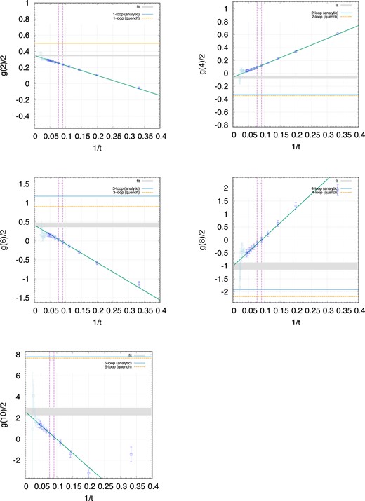
Obtained values of g(t → ∞)/2 are plotted for four choices of mγa in Fig. 4. Three points mγ/m = 0.4, 0.5, 0.6 are used for the linear extrapolation to mγ = 0 while fixing m. Expected systematic uncertainties by this extrapolation are on the order of 20%–30% due to higher-order terms in the mγ expansion, i.e. |$\mathcal {O}(m_{\gamma }^2/m_f^2)$|. The effects of the discretization are expected to be larger for higher orders in perturbations. In addition to the discretization effects of O(m2a2), the UV cutoff in the photon kinetic term gives corrections typically,
as a multiplicative factor for each photon propagator. For a choice of too small Λ/m, we obtain exponentially suppressed values. The choice of Λ2 = 4.0 seems to be not too small. Further large values, however, make the statistical error larger and also the logarithmic correction larger. One should look for optimal values of Λ for different choices of simulation parameters.
![Extrapolation to mγ = 0 on the 243 × 48 lattice. Horizontal lines show the results from Feynman diagram computations (at k2 = 0 and mγ = 0). For the five-loop coefficient, the solid line shows the result of Refs. [2,21] while the dashed one the result of Ref. [3]. In the first panel, the solid curve represents the finite photon mass correction theoretically calculated in Eq. (51) (while setting k2 = 0) in continuum spacetime.](https://oup.silverchair-cdn.com/oup/backfile/Content_public/Journal/ptep/2023/10/10.1093_ptep_ptad125/3/m_ptad125fig4.jpeg?Expires=1750200193&Signature=QQpn2usn4~fH215wfX0Y~Z8qzFKSWQF~1-nILh94RpGweXisn4lSwAXZKMG3rEJnDwKPHmWH7FYF5OqLfRJbqjci8B~JO6lsKYXxL4Jiu48lpyhH8paoYiuIe5EEvZjOTf8y66srUjLF578SO1Nd0bL8do3iaMROSQ6L2IrxBb~qU~uz9~NcXnY3A~DaSiUfdVHmuHVodyqjH6TIzkDcjklHqEilbULim0NAbeKhtlMICNs6qyBF4bFM8fk335bxda-jU4kwKEPciOg026yWRslQNIiyxyVgcnwjakZz8V0-23y5-TPXZZIE~R3F~RYhAA3tu-xan7LPk50B1U7DaA__&Key-Pair-Id=APKAIE5G5CRDK6RD3PGA)
Extrapolation to mγ = 0 on the 243 × 48 lattice. Horizontal lines show the results from Feynman diagram computations (at k2 = 0 and mγ = 0). For the five-loop coefficient, the solid line shows the result of Refs. [2,21] while the dashed one the result of Ref. [3]. In the first panel, the solid curve represents the finite photon mass correction theoretically calculated in Eq. (51) (while setting k2 = 0) in continuum spacetime.
We show the analytic results of g/2 with finite photon masses at the one-loop level (using the first equality of Eq. (51) with k2 = 0) in Fig. 4 as the solid curve. The lattice results are significantly off the line, which represents the discretization effects. With the finite photon mass, there can be discretization errors on the order of mγa in addition to m2a2. Therefore, the limit of mγ → 0 would give the closest value to the continuum theory. Such a tendency can be seen in the figure.
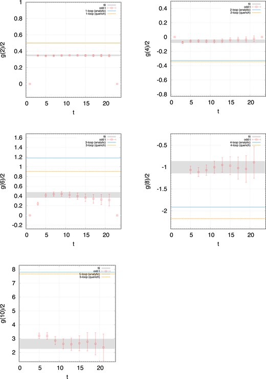
We repeat the same analyses for L = 20, 18, 16, and 14, while keeping mγ/m = 0.4−0.7 and mγL = 4 for the smallest mγ as listed in Table 1. For smaller lattices, the fermion mass ma is larger, and thus results are further from the continuum limit. We show in Fig. 5 the m2a2 dependence of the g factor on each lattice. We see the tendency of approaching toward the correct values.5
![The continuum limit. For the five-loop coefficient, the solid line shows the result of Refs. [2,21] while the dashed one the result of Ref. [3].](https://oup.silverchair-cdn.com/oup/backfile/Content_public/Journal/ptep/2023/10/10.1093_ptep_ptad125/3/m_ptad125fig5.jpeg?Expires=1750200193&Signature=o98Y-5Ca8XzhHnTNsBYDQ1RLtnPVeUHlYZyYVqESWvyrBWVVhkPOq2AER6jiA00~fmmeDAL06RgrgzkLUk4--JjJdP97D8FGCNLz0Zugs6ZKBikSjPUL1JWy-CWkXj0y6PZjSjCanKznJq4E4fKIU9-Uh9a1XQe5PMyRdqmP81i7w3LodBed6Fz61J~RwuHL0H~gMQidrweY-GygxDci56kwVFgSU~Cj~xpzkdZ4wXmuNlHFZR2MMwJaU854Yij5-B5AdCcsru1wx8wmnRMZeJxrtAgbXtJkE17wPhTMOV3uqBpDM~nNGpWwwjetYMTddj6W-f2cP~Rj8x2mJ2p4Cg__&Key-Pair-Id=APKAIE5G5CRDK6RD3PGA)
We refrain from presenting the values of our result because they are not conclusive ones; as we noted, the photon mass cannot be taken small enough in the present study, and the extrapolation to mγ → 0 can have large errors. For instance, the data point at mγ/m = 0.4 for g(2) has an error of ∼40%, as seen from the first panel in Fig. 4. The detailed study of systematic uncertainties is skipped in this work accordingly.
Although the statistical uncertainties are large, the calculation up to the five-loop level seems to be doable in a larger-scale simulation. For L = 128, e.g. one can take mγ/m = 0.1 and m2a2 = 0.1 while satisfying mγL = 4. This would significantly reduce the uncertainties of the mγ → 0 extrapolation.
4. Conclusions and discussion
In this paper, aiming at giving the five-loop coefficient of the electron g factor using the lattice, we developed a theoretical study of FV corrections and also performed a numerical simulation using small lattices. We first studied FV corrections in various IR regularization methods of lattice QED to discuss the optimal regularization for our purpose. We found that in QEDL FV corrections to the effective mass can have different parametric dependences depending on the size of Euclidean time t. The ‘naive on-shell result’ turns out to be valid only for t ≫ L. We also discussed a possible method to make the FV correction smaller than ∼1/(mL). In contrast to such complexity in QEDL, finite photon mass regularization seems to always suppress FV corrections exponentially |$\sim e^{-m_{\gamma } L}$|. We therefore adopted finite photon mass regularization.
In addition to FV effects, we studied corrections to the g factor due to finite photon mass and finite photon momentum k2. We gave the parametric dependences on these perturbations; this understanding is used to fix extrapolation functions. Based on these studies on systematic errors, we presented an optimal strategy for selecting the simulation parameters |$m_{\gamma }, m, \Lambda _{\rm UV}^2, L$| and the order of various extrapolations.
We presented a numerical lattice simulation following our strategy. Due to the limited lattice volume in our study, the evaluation of the systematic uncertainties, such as those in the mγ → 0 and a → 0 extrapolations, needs more study. With our choice of parameters, we observed large discretization effects. This can be understood from discretization effects of |$\mathcal {O}(m_{\gamma } a)$|; we could not take small enough mγ due to the smallness of the lattices. Apart from this, we made several important observations. Firstly, we observed a clear linear dependence in 1/t for g(t) (see Figs. 2 and 3). This behavior can be understood as a consequence of the suppression of backward propagation and the suppression of FV corrections (owing to mγL ≫ 1). When FV corrections are not suppressed enough, higher poles appear in Fourier-transformed quantities and disturb a linear t dependence as discussed in Ref. [7]. Secondly, we observed that the discretization effect for the g factor is consistent with a linear dependence in (ma)2 as theoretically expected (see Fig. 5), yet the statistical precision and the mγ → 0 extrapolation need to be improved.
The photon mass can be taken small when large lattices are available and discretization effects will be improved significantly. We estimated that the required size is L ∼ 128. We would like to update our results using larger lattices in the future.
Acknowledgement
The authors would like to thank Masashi Hayakawa for discussions. The work is supported by Japan Society for the Promotion of Science (JSPS) KAKENHI Grant Numbers JP19H00689 (R.K.), JP19K14711 (H.T.), and JP21H01086 (R.K.) and Ministry of Education, Culture, Sports, Science and Technology (MEXT) KAKENHI Grant Number JP18H05542 (R.K., H.T.).
Funding
Open Access funding: SCOAP3.
Appendix. Branch cut contribution to the effective mass
We consider scalar QED:
with
The two-point function of the renormalized scalar field is given to the one-loop level by
where
with
Πana is analytic at |$p^2=-\overline{m}^2$| and Πcut has a branch cut starting at |$p^2=-\overline{m}^2$|. We consider the |$\overline{\rm MS}$| renormalization and |$\overline{m}$| denotes the |$\overline{\rm MS}$| mass. We work at the Feynman gauge. One can interpret the |$\overline{\rm MS}$| mass as the tree-level mass in terms of perturbative QED.
The Euclidean time correlator is given by
We take p = (0, 0, 0, p4). Let Cana and Ccut be the first and second lines of the last equality of Eq. (A7), respectively. If we approximate Πcut as |$\Pi ^{\rm cut}(p^2)\simeq -\frac{\alpha }{\pi } (p^2+\overline{m}^2) \log \left(\frac{p^2+\overline{m}^2}{\overline{m}^2} \right) =:\tilde{\Pi }^{\rm cut}(p^2)$| focusing on the point |$p^2=-\overline{m}^2$|, we have an approximated result of the second line of Eq. (A7):
Here Ka is the Bessel function of the second kind. In giving the above result, we used
and took the derivative with respect to ϵ. Our numerical analysis shows that the logarithmic term in Eq. (A8) is dominant for |$\overline{m}t \gg 1$|. We expect that the behavior of Πcut at |$p^2=-\overline{m}^2$| is the same for composite particles because it is determined by the IR photon.
In Fig. A1, we give the effective mass extracted from the Euclidean time correlator C(t) (blue) and the one from |$C(t)-\tilde{C}^{\rm cut}(t)$| (green). We give C(t) numerically (by a numerical evaluation of the second line of Eq. (A7)), while we use the analytic result (A8) for |$\tilde{C}^{\rm cut}(t)$|. The blue line corresponds to ‘lattice data’ and the green one corresponds to ‘corrected lattice data’. The green line lies much closer to the exact pole mass value (black) than the blue line. This would imply that the effective mass can be accurately obtained even at the relatively small t region by removing the cut effect evaluated as Eq. (A8).
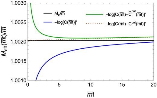
Analyses of the effective mass. We show the straightforward analysis result (blue) and a cut-associated contribution–subtracted result (green). We take the renormalization scale |$\mu =\overline{m}$| and α = 1/137.
We make a remark regarding the figure. If we eliminate the cut effect best, i.e. extract the effective mass from C(t) − Ccut(t) (where Ccut is also evaluated numerically), we obtain the dotted line. This line has a small slope and does not generally agree with the pole mass value. This deviation can be understood as higher-order [|$\mathcal {O}(\alpha ^2)$|] effects and thus an artifact of truncated perturbation theory.
Footnotes
One can prove κ−2 = κ−3/2 by rewriting the integrals |$\int _0^{\infty } ds =[\int _0^1+\int _1^{\infty }] ds$| by |$\int _0^1 ds$| integrals and using Eq. (6).
The s-integral can be decomposed into |$\int _0^{\infty }ds=\int _0^1 ds+\int _1^{\infty } ds$|. While the integral |$\int _1^{\infty } ds$| gives an expansion in |$2 m_f^2/\Lambda _{\rm UV}^2$|, the integral |$\int _0^1 ds$| can give a |$2 m_f^2/\Lambda _{\rm UV}^2 \log (2 m_f^2/\Lambda _{\rm UV}^2)$| term.
We neglect mγa in this discussion.
Due to the smallness of the expansion coefficient in |$k^2/m_f^2$| in Eq. (51), the error of the k2 = 0 extrapolation is expected to be small. The careful study of this systematic uncertainty requires more data points and will be our future work.
For g(8) and g(10), the data points are not fitted well in Fig. 5. We consider that this is due to the large systematic error in the mγ → 0 extrapolation, as mγ cannot be taken small enough in this study. Note that the data points only have statistical uncertainties.
