


Abstract
The third-order structure resonance due to sextupole magnetic fields was compensated in the Japan Proton Accelerator Research Complex main ring synchrotron using new beam optics. In the present optics, the third-order structure resonance νx − 2νy = −21 was so strong that the working point was limited. The new optics cancels the resonance by adjusting the phase advances in the arc sections. The resonance compensation was verified by aperture survey simulations and further demonstrated by three types of experiment. First, transverse coupling measurements were performed. The coupling was observed only for the optics without the compensation. This was also verified with the tracking simulation. Second, beam losses were measured using the current and new optics. The measured beam losses were noticeably reduced at the tunes around the resonance using the new optics. The beam loss reduction was also verified with the space charge tracking simulation. Third, Fourier analyses of the transverse dipole oscillations were conducted for both optics. Fourier spectra derived from the resonances were observed, and their peaks were clearly suppressed with the new optics. This was also consistent with the results of the space charge simulations.
1. Introduction
In circular accelerators, low-order resonances limit the available tune region. In particular, third-order resonances driven by the sextupole magnetic fields exist in nearly every synchrotron. In large synchrotrons that use sextupole magnets to correct the chromaticity, the magnets can cause third-order resonances. Even in synchrotrons that do not use sextupole magnets, the sextupole field components of the bending magnets can drive third-order resonances.
Methods for suppressing third-order resonances have been studied extensively. There are a number of studies reporting the compensation of nonstructure resonances, such as Refs. [1–4]. They compensated for the third-order nonstructure resonances by applying additional sextupole magnetic fields or by changing the strengths of the sextupole magnets. Unlike nonstructure resonances, there is a small number of references for the compensation of structure resonances. In many cases, structure resonances are too strong to be compensated using corrector sextupole magnets. One example for suppressing the effect of the third-order structure resonance was proposed in Ref. [5]. They found that the emittance growth by the νx − 2νy = n resonance, known as the Walkinshaw resonance [6], can be minimized by setting the transverse emittance according to 2εx = εy.
In this study we propose a new method to compensate for the third-order structure resonance [7]. Our technique does not require additional corrector sextupole magnets and does not impose constraints on the beam distribution. The requirement for our compensating method is symmetry of the arc section of the synchrotron. Figure 1 shows a schematic of the main ring synchrotron (MR) of the Japan Proton Accelerator Research Complex (J-PARC) [8], where we demonstrated the effectiveness of the compensation method [7]. In the J-PARC MR, one arc section is composed of eight symmetric structures. Our compensation method cancels the third-order structure resonance by properly adjusting the phase advance in the arc sections. The tune can be maintained by adjusting the straight sections. The detailed theory is described in the next section.
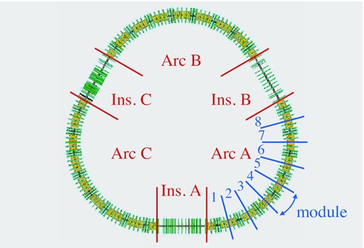
Schematic of the J-PARC MR, which consists of three straight (insertion) sections and three arc sections. One arc section is composed of eight symmetric modules.
The J-PARC MR is a proton synchrotron with three-fold symmetry of the focusing lattice delivering 30 GeV protons for neutrino and hadron experiments. At present, the average beam power is 515 kW for neutrino and 65 kW for hadron experiments. The beams are injected with a kinetic energy of 3 GeV and an intensity of 3.3 × 10¹³ protons per bunch (ppb). In total, eight bunches are injected within 130 ms and then the beams are accelerated to 30 GeV. In the present neutrino user operation conditions, the tune is set to (νx, νy) = (21.35, 21.43) [9,10]. The relevant parameters for neutrino user operation are presented in Table 1.
Typical parameters in neutrino user operation.
| Circumference C | 1567.5 m |
| Superperiod | 3 |
| Harmonic number | 9 |
| Number of bunches | 8 |
| Ring aperture | >81π mm mrad |
| Collimator aperture | ∼60π mm mrad |
| Injection energy | 3 GeV |
| Extraction energy | 30 GeV |
| Injection period | 130 ms |
| Cycle time | 2.48 s (0.403 Hz) |
| Tune (νx, νy) | (21.35, 21.43) |
| Chromaticity (ξx, ξy) | (−7, −7) |
| Transition energy γT | i31.7 |
| Beam intensity | 3.3 × 10¹³ ppb |
| Beam power | 515 kW |
| Beam loss | 0.8 kW |
| Injection geometric emittance (εrms, x, εrms, y) | (4.6π, 4.8π) mm mrad |
| Injection bunching factor Bf | 0.2 |
| Injection momentum spread σδ | 0.0016 |
| Maximum tune shift ΔνSC | −0.34 |
The beam power is planned to be upgraded to 1.3 MW for neutrino and to 100 kW for hadron experiments [4,11]. The upgrade plan assumes a hardware upgrade for faster cycling and higher intensity, and relies on lower beam losses in operation. Beam loss reduction is a general concern in high-intensity proton and ion accelerators, such as the Fermilab Booster and Main Injector [12–15], CERN PSB, PS, and SPS [16–20], AGS at BNL [21], ISIS at RAL [22], SIS18 at GSI [23], and CSNS/RCS [24]. The beam loss in the MR is strongly related to space charge effects [4,9,–11]. Most of the beam losses can be observed in the first 300 ms, where the beam energy is below 5 GeV. In this period, the space charge effect is strongest, resulting in a large tune spread ΔνSC ≃ −0.34.1 The particle-in-cell tracking simulation software Space Charge Tracker (SCTR) [25,26] indicates that the protons are lost because of resonance crossings [9,–,11].
In the J-PARC MR there are seven kinds of quadrupole electromagnets in the straight sections and four kinds in the arc sections. The same kinds of magnets have the same structures, and their magnet currents are from the same power supply. The quadrupole magnets in the arc sections are carefully set to realize an achromat lattice, and their currents are rarely changed after adjustment. The fine tuning of the working point is performed only by the quadrupole magnets in the straight sections.
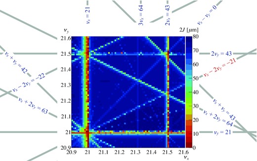
Figure 2 shows the result of an aperture survey simulation near the working point in neutrino user operation. The initial actions of the particles which did not hit the aperture were investigated by tracking simulations. The strengths of the resonances can be seen. Since the MR has three-fold symmetry, the third-order structure resonances appear at νx = 21, νy = 21, νx − 2νy = −21, and νx + 2νy = 63 in Fig. 2. While the integer resonances are excited by several kinds of effects [27], the νx − 2νy = −21 and νx + 2νy = 63 resonances are induced by the sextupole magnetic fields in the sextupole and bending magnets. These resonances appear even if there are no imperfections of the magnets. Some resonances emerge when there are magnet imperfections, known as nonstructure resonances. For example, the third-order nonstructure resonances 3νx = 64 and νx + 2νy = 64 can be seen in Fig. 2. Although the magnet imperfections also affect the νx − 2νy = −21 and νx + 2νy = 63 resonances, their effects are almost hidden because the structured effects are much stronger.
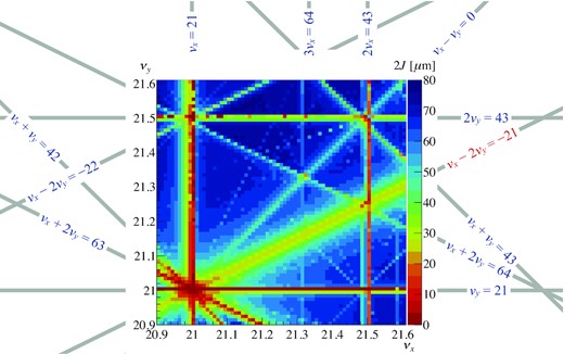
Aperture survey simulation around the present neutrino user operation. Particles with transverse actions of 2Jx = 2Jy = n μm (n = 0, 1, 2, …) and with the zero longitudinal amplitude were prepared. Single-particle tracking was performed for each particle. The figure shows the maximum initial actions of the particles that survived during tracking. We judged that the particle was alive if its action did not exceed 81π mm mrad, which is the physical aperture in the MR. Alignment and magnetic field gradient errors were applied, while space charge effects were not included. The closed orbit was corrected in every tune. The related parameters are shown in Table 2.
From the next section, the compensation of third-order structure resonances is discussed. In Sect. 2, the theory of the compensation method is described. From Sect. 3, the application to the J-PARC MR is discussed. In this paper we focus on the third-order structure resonance νx − 2νy = −21. In Sect. 3, we verify the compensation by aperture survey simulations. The compensation method is demonstrated by three types of measurement: via transverse coupling measurements in Sect. 4, via beam loss measurements in Sect. 5, and via the Fourier spectra of dipole oscillations in Sect. 6. The discussion is concluded in Sect. 7.
2. Principle of compensation
We suppose that the sextupole magnets are located in the arc sections. Since the bending magnets are also located in the arc section, the resonance driving terms of the third-order structure resonances arise in the arc sections.
Figure 3 shows images of the compensation of G1, −2, l in the case of M = 8. The left image shows the resonance driving terms without the compensation, assuming the present optics for neutrino user operation. The phase advance per module is Δψmod, x − 2Δψmod, y = −2π(11/16), which does not satisfy Eq. (14). As a result, each resonance driving term per module, represented by a black vector, points in a different direction. The resonance driving term in one arc section appears as the sum of those, indicated by the red vector. The case of the compensation optics is shown on the right. In this case we assume Δψmod, x − 2Δψmod, y = −2π(5/8), which corresponds to (j, M) = (−5, 8) in Eq. (14). All the black vectors have the same norm, and their directions are now isotropic. As a result, the sum of the vectors becomes zero and the resonance is compensated.
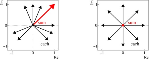
Schematic illustrations of the compensation method. The left and right images show the resonance driving terms without and with compensation, respectively. The black vectors represent the resonance driving terms in one module. The red vector, which is the sum of the black vectors, represents the resonance driving term in one arc section. In the right image, the sum of the vectors is zero.
3. New optics for the J-PARC MR
As shown in Fig. 1, the number of superperiods in the MR is N = 3, and the number of modules in one superperiod is M = 8. All sextupole magnets are located in the arc sections.
Since the number of modules in one superperiod is M = 8, the horizontal phase advance of one arc section is Δψarc, x = 8Δψmod, x = 12π in the present optics. The horizontal phase advance Δψarc, x was carefully adjusted such that the arc section became achromat. The optics was verified by measurements of the betatron functions and dispersions [29,30]. Moreover, the present phase advance satisfies the condition for compensation of the resonance driving term G3, 0, n given in Eq. (13). Therefore, the horizontal phase advance Δψmod, x should not be changed. On the other hand, there were no restrictions for the vertical phase advance Δψmod, y.
The betatron functions of the present and new optics are shown in Fig. 4, and are not significantly different. This means that the physical apertures do not change dramatically in the action coordinates. The betatron functions and the dispersion function were also measured with the new optics, as described in Appendix B.
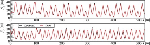
Horizontal (top) and vertical (bottom) betatron functions with the present (black) and new (red) optics in a superperiod. The straight section is s = 0–116.1 m and the arc section is s = 116.1–522.5 m.
The aperture survey simulation was also performed with the new optics to verify the compensation. The tune was changed by maintaining the phase advance in the arc sections. In other words, the tune was adjusted only by the quadrupole magnets in the straight sections. The strengths of the sextupole magnets were fixed. The resonance driving terms must not have changed during the tune scan, because the phase advance in the arc sections and the strengths of the sextupole magnet fields were fixed.
Figure 5 shows the results of the aperture survey simulation with the new arc optics. Compared with the results of the present arc optics shown in Fig. 2, it is obvious that the νx − 2νy = −21 resonance was compensated. The values used in the aperture survey simulation are listed in Table 2.
Aperture survey simulation with the new optics. The phase advances in the arc sections were unchanged throughout the simulation. Alignment and magnetic field gradient errors were included. The related parameters are shown in Table 2.
Values used in the aperture survey simulations. The alignment and magnetic field gradient errors were included to reproduce the measurements of the nonstructure resonance driving terms G3, 0, 64 and G1, 2, 64.
| Present | New | |
|---|---|---|
| Physical aperture | 81π mm mrad | |
| Beam energy | 3 GeV | |
| Turn | 1000 | |
| Phase advance per module (Δψmod, x, Δψmod, y) | |$2\pi \left(\frac{3}{4}, \frac{23}{32}\right)$| | |$2\pi \left(\frac{3}{4}, \frac{11}{16}\right)$| |
| Tune (νx, νy) | (20.9–21.6, 20.9–21.6) | |
| Tune step | 0.01 | |
| Accuracy of the tune | <0.002 | |
| Chromaticity (ξx, ξy) | (−6, −7) | (−6, −7) |
| G1, −2, −21 (structure) | 3.68 m−1/2 | 0.10 m−1/2 |
| G3, 0, 64 (nonstructure) | 0.07 m−1/2 | 0.04 m−1/2 |
| G1, 2, 64 (nonstructure) | 0.15 m−1/2 | 0.17 m−1/2 |
According to Eq. (13), the new arc optics compensate not only the resonance driving term G1, −2, n but also G1, 2, n. The corresponding resonance shown in Figs. 2 and 5 is νx + 2νy = 63. Comparing the two results, it can be verified that the νx + 2νy = 63 resonance was also compensated.
In the result of the aperture survey simulation for the new arc optics, the νx − 2νy = −21 resonance can be seen slightly. This is because it was driven by imperfections of the magnets. In other words, the νx − 2νy = −21 resonance existed as a “nonstructure” resonance.
4. Verification of the compensation by coupling measurements
The compensation for the third-order structure resonance νx − 2νy = −21 was verified not only by the aperture survey simulations but also using three types of experiment. First, the transverse coupling was measured. The νx − 2νy = −21 resonance couples horizontal and vertical motions of the beam.
To observe the transverse coupling the turn-by-turn transverse beam positions were measured. The beams were intentionally injected with dipole errors in the horizontal plane. While in the vertical plane, the beams were injected without dipole errors. The tune was set at (νx, νy) = (21.44, 21.22), where the beam was on the νx − 2νy = −21 resonance. If the beam is affected by the νx − 2νy = −21 resonance, the horizontal dipole oscillation propagates to the vertical plane.
4.1. Simulation prediction
Initial conditions of the simulations for the coupling measurements.
| Beam energy | 3 GeV |
| Beam intensity | 2.5 × 10¹² ppb |
| Tune (νx, νy) | (21.44, 21.22) |
| Chromaticity (ξx, ξy) | (−3, −3) |
| Transverse distribution | Gaussian |
| Emittance (εrms, x, εrms, y) | (1.0π, 1.0π) mm mrad |
| Longitudinal distribution | Parabola |
| Bunching factor Bf | 0.17 |
| Momentum spread σδ | 0.0016 |
Figure 6 shows the results of the turn-by-turn actions obtained from the simulations. The vertical action became larger in the present arc optics, although it was initially zero. This is because the transverse dipole motions were coupled, and the horizontal amplitude propagated to the vertical plane. In the new arc optics, no noticeable dipole oscillation was seen in the vertical plane. This indicates that the νx − 2νy = −21 resonance was compensated for in the new arc optics. The oscillations were damped by the effects of the chromatic tune spread and space charge.
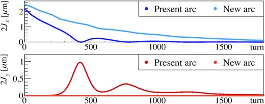
Action as a function of the turn obtained from the simulations. The top image shows the horizontal and the bottom image the vertical action. The results for the present arc optics are represented by the blue (horizontal) and red (vertical) lines. The results for the new arc optics are represented by the sky blue (horizontal) and orange (vertical) lines.
The tune dependence of the coupling was also studied. Figure 7 shows the turn-by-turn vertical actions in the present arc optics. The different colors correspond to the different tunes. In the top figure, the vertical tunes are fixed at νy = 21.22. It indicates that the coupling may not be measured if the horizontal tune is shifted by 0.006. In the MR, the tune itself fluctuates (see Appendix B), and the typical fluctuation amplitude is 0.005. It can be predicted that the turn-by-turn motions will differ shot by shot. The bottom figure shows the vertical tune dependence. In these simulations, the horizontal tunes were fixed at νx = 21.44. The results indicate that the vertical tune is more sensitive to the coupling than the horizontal tune. This can be attributed to the resonance proximity parameter δ ≡ νx − 2νy + 21 [28]. The vertical tune νy is twice as effective as the horizontal tune νx on δ.
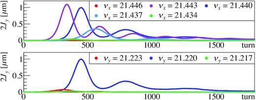
Horizontal (top panel) and vertical (bottom panel) tune dependence of the turn-by-turn vertical actions using the present arc optics from simulations. In the top image, the vertical tunes are fixed to νy = 21.22. In the bottom image, the horizontal tunes are fixed to νx = 21.44.
4.2. Coupling measurements
The coupling was also observed in the measurements. The turn-by-turn transverse beam positions were measured by the beam position monitors (BPMs) [31–33]. In the same way as the simulations, the beams were injected with dipole errors in the horizontal plane, and the vertical dipole errors at the beam injection were carefully corrected. The tune was set at (νx, νy) = (21.44, 21.22). Low-intensity beams were used to suppress the space charge effects.
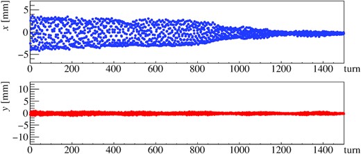
Figure 8 shows the results of the turn-by-turn beam positions using the present arc optics. It is clear that the horizontal and vertical dipole oscillations were coupled. On the other hand, Fig. 9 shows the results using the new arc optics. The amplitude of the vertical dipole oscillation was maintained at approximately 1 mm. No clear coupling was seen.

Turn-by-turn beam positions with a tune of (νx, νy) = (21.44, 21.22) with the present arc optics. The top image shows the horizontal positions and the bottom image the vertical.
Turn-by-turn beam positions with a tune of (νx, νy) = (21.44, 21.22) with the new arc optics. The top image shows the horizontal positions and the bottom image the vertical.
In these experiments, as predicted, the dipole oscillations varied shot by shot. Even when using the present arc optics, the couplings were not seen in some results. This was because the dipole oscillations were very sensitive to the tune, as indicated by the simulations. The shot-by-shot differences can be explained by the fluctuations in the tunes.
To cope with the shot-by-shot differences, the dipole oscillations were measured many times under the same conditions. We judged whether the coupling occurred by checking that the amplitude of the vertical position was greater than 3 mm. Since the betatron function at the BPM used was βy = 26.5 m in the new arc optics, the 3 mm amplitude corresponds to the action of |$2J_y = 0.34 \, \mu$|m.
Table 4 shows the results of the coupling measurements. We defined the “coupled event ratio” as the ratio of the number of coupled events to the total number of events. In the new arc optics, coupling was not observed in any measurements. It is clear that the νx − 2νy = −21 resonance was compensated in the new arc optics.
Results of the coupling measurements with the beam conditions. The tunes are the measured values.
| Optics | Intensity | Tune | Chromaticity | Coupled event ratio |
|---|---|---|---|---|
| (νx, νy) | (ξx, ξy) | |||
| Present | 1.2 × 10¹² ppb | (21.440, 21.227) | (−0.4, −0.5) | 4/10 (40%) |
| (−1.5, −1.6) | 5/10 (50%) | |||
| (−2.9, −3.1) | 3/10 (30%) | |||
| 2.5 × 10¹² ppb | (21.437, 21.221) | (−7.4, −7.7) | 17/20 (85%) | |
| New | 2.5 × 10¹² ppb | (21.440, 21.218) | (−7.4, −7.8) | 0/15 (0%) |
| (−2.9, −3.2) | 0/10 (0%) |
Figure 10 shows the actions 2Jx, 2Jy as a function of the turn in the present arc optics. The data shown in Fig. 10 are the same as in Fig. 8. It is clear that the horizontal and vertical actions were coupled with each other.
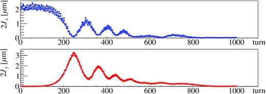
Turn-by-turn actions using the present arc optics. The top image shows the horizontal action 2Jx, and the bottom image shows the vertical action 2Jy. The data shown in the figure are the same as in Fig. 8.
Ideally, the value Jc = 2Jx + Jy is constant, but this equation neglects the damping effects of the dipole oscillations. As can be seen in Figs. 8 and 10, the dipole oscillations were damped in the real measurements. This indicates that the value Jc was also damped. However, since the speed of the damping was not very fast, Jc can be considered constant over a short time scale. Figure 11 shows the relationship between the transverse actions. The plots are colored according to the number of turns. The motions of turn numbers 160–309, shown as blue circles, were on the line |$2J_x + J_y = 1.7 \, \mu$|m. Similarly, the motions of turn numbers 310–424, shown as sky blue circles, were on the line |$2J_x + J_y = 1.2 \, \mu$|m. The motions of turn numbers 425–494, shown as green circles, were on the line |$2J_x + J_y = 0.75 \, \mu$|m. Thus, the Jc = 2Jx + Jy value was constant over a short time range. This reveals that the source of the coupling is the νx − 2νy = −21 resonance.
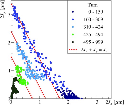
Turn-by-turn actions with the present arc optics in the 2Jx − 2Jy coordinates. The colors indicate the number of turns: dark blue for turn numbers 0–159, blue for turn numbers 160–309, sky blue for turn numbers 310–424, green for turn numbers 425–494, and dark green for turn numbers 495–999. The additional three red dotted lines show the conditions 2Jx + Jy = Jc with different Jc values. From the top, |$2J_c = 3.4\, \mu$|m, |$2J_c = 2.4\, \mu$|m, and |$2J_c = 1.5\, \mu$|m. The data shown in the figure are the same as in Figs. 8 and 10.
5. Verification of compensation by beam loss measurements
The second experiment for the verification of the compensation for the third-order structure resonance νx − 2νy = −21 involved beam loss measurements. If the νx − 2νy = −21 resonance is compensated, the beam loss due to the resonance is reduced. We compared the beam losses of the present and new arc optics. The tune was scanned across the νx − 2νy = −21 resonance to confirm that the resonance caused the beam loss.
Figure 12 shows the major resonances and the scanned range, which was νy = 21.20–21.29. The horizontal tune was fixed at νx = 21.44. Other resonances can also cause beam losses. A significant resonance was the third-order nonstructure resonance 3νx = 64, because it could affect many particles considering the space charge tune shift. To suppress its effect, the two nonstructure resonances 3νx = 64 and νx + 2νy = 64 were compensated by using the trim coils of the sextupole magnets [4,9]. The reason for fixing the horizontal tune is to consider the residual nonstructure resonance. Even if a residual nonstructure resonance 3νx = 64 arises, its effects do not change during the scan.
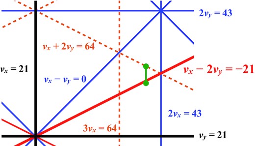
Scanned range in the tune diagram. The scanned range, shown as the green line, was (νx, νy) = (21.44, 21.20–21.29).
5.1. Experiments
Table 5 lists the conditions used in the experiments. The collimator aperture was set to be small to observe the beam losses clearly. The position of the collimator, determined based on the betatron functions at the vertical tune νy = 21.24, was fixed during the tune scan. The setting values were calculated by using the Strategic Accelerator Design (SAD) [34] computer program. The betatron functions at the position of the collimator calculated by SAD were (βx, βy) = (20.79, 10.06) m for the present arc optics and (βx, βy) = (23.30, 8.08) m for the new arc optics. The maximum beta deviations resulting from the change of the optics during the tune scan were |$(|\Delta \beta _x|/\beta _x, |\Delta \beta _y|/\beta _y) = (0.8\%, 2.4\%)$| for the present arc optics and |$(|\Delta \beta _x|/\beta _x, |\Delta \beta _y|/\beta _y) = (0.4\%, 1.1\%)$| for the new arc optics.
Conditions for the beam loss scan experiments.
| Number of bunches | 2 |
| Horizontal aperture | 40π mm mrad |
| Vertical aperture | 40π mm mrad |
| Beam energy | 3 GeV |
| Circulating time | 130 ms |
| Horizontal tune νx | 21.44 |
| Vertical tune νy | 21.20–21.29 |
| Chromaticity (ξx, ξy) | (−7, −7) |
| Beam intensity | 2.3 × 10¹³ ppb |
| Number of bunches | 2 |
| Horizontal aperture | 40π mm mrad |
| Vertical aperture | 40π mm mrad |
| Beam energy | 3 GeV |
| Circulating time | 130 ms |
| Horizontal tune νx | 21.44 |
| Vertical tune νy | 21.20–21.29 |
| Chromaticity (ξx, ξy) | (−7, −7) |
| Beam intensity | 2.3 × 10¹³ ppb |
A direct-current current transformer (DCCT) [31,32,35,36] was used to obtain the beam losses. The beam current can be measured by the DCCT in the MR with an accuracy of 1% [35] and a relative deviation of 0.1% [36]. The time resolution is about 100 μs and is short enough compared to the circulating time of 130 ms.
The experiments were conducted with relatively high-intensity beams to observe clear responses of beam losses. The low-intensity beams were not lost because their emittances were small. In the MR, the transverse emittance at the beam injection was nearly linear with respect to the beam intensity [11]. The beam intensity was scanned and set to 2.3 × 10¹³ ppb because the beam loss with the present arc optics was about 10% which was larger than the DCCT accuracy. The chromaticity setting was the same as for neutrino user operation. The distortions of the closed orbit were less than 1 mm at every point. The injection beta matching was performed by scanning the quadrupole magnets in the beam transport line.
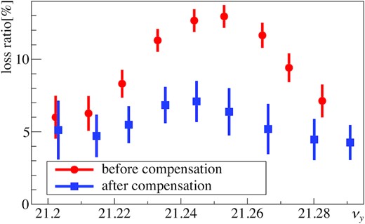
Figure 13 shows the results of the beam loss ratios, defined as the ratio of the decrease of the beam current in 130 ms measured by the DCCT. The tunes were measured by the tune meter [31,32] using weak-intensity beams (2.5 × 10¹² ppb). In the results for the present arc optics, the beam loss reached its peak at νy = 21.24–21.25. For the new arc optics, the peak was suppressed compared to the present arc optics. These show that the νx − 2νy = −21 resonance was successfully weakened.
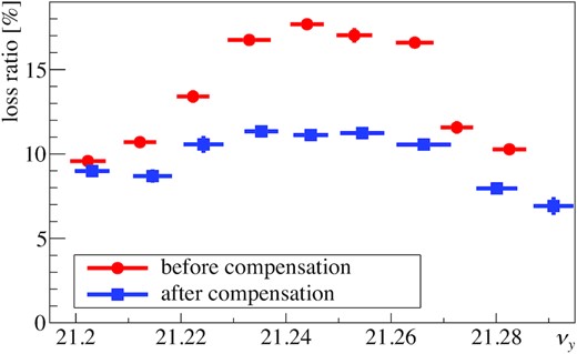
Beam losses in the present (red) and new (blue) arc optics. The horizontal axis shows the measured vertical tune. The horizontal error bars represent the oscillations of the vertical tunes. The vertical error bars represent statistical errors. The systematic errors are not shown in this figure.
Although the on-resonance condition was νy = 21.22, the peak was at νy = 21.24–21.25. This was due to the space charge detuning. Since the horizontal and vertical emittances are nearly the same in the MR, the peak of the loss was shifted above the resonance.
Ideally, the peak due to the νx − 2νy = −21 resonance is flattened in the new arc optics. The small peak in the new arc optics was derived from imperfections of the magnets. This indicates that the structure resonance was compensated, but the νx − 2νy = −21 resonance remained as a nonstructure resonance. This can be compensated by using the trim coils of the sextupole magnets, if needed.
5.2. Simulations
Resonance compensation using the beam loss scan was also performed using SCTR simulations. In these simulations, the particles were lost when their actions became larger than the aperture. The conditions were set to be the same as those in the experiments; they are listed in Table 6.
Conditions for the beam loss scan simulations.
| Horizontal aperture (present) | 38.6π ± 2.7π mm mrad |
| (new) | 38.2π ± 2.6π mm mrad |
| Vertical aperture (present) | 39.6π ± 4.0π mm mrad |
| (new) | 36.5π ± 4.2π mm mrad |
| Beam energy | 3 GeV |
| Circulating time | 24 200 turns (130 ms) |
| Horizontal tune νx | 21.44 |
| Vertical tune νy | 21.20–21.29 |
| Beam intensity | 2.3 × 10¹³ ppb |
| Initial transverse distribution | Gaussian |
| Initial emittance (εrms, x, εrms, y) | (4.2π, 4.2π) mm mrad |
| Initial longitudinal distribution | Parabola |
| Initial bunching factor Bf | 0.21 |
| Initial momentum spread σδ | 0.0017 |
| Number of macro particles | 200 000 |
In the experiments, there were systematic shifts due to the distortions of the closed orbits at the collimator. Using the BPMs near the collimator, the distortions were estimated as (Δx, Δy) = (0.5, 0.1) mm for the present arc optics, and (Δx, Δy) = (0.7, 0.8) mm for the new arc optics. The distortion decreased the effective aperture size. The effective aperture was estimated as (H,V) = (38.6π, 39.6π) mm mrad for the present arc optics, and (H,V) = (38.2π, 36.5π) mm mrad for the new arc optics. The distortions of the closed orbits were slightly different shot by shot. In addition, the collimator position had certain errors. The error in the distance between the beam and the collimator was assumed to be 0.5 mm. This corresponds to aperture errors of (H,V) = (2.7π, 4.0π) mm mrad for the present arc optics, and (H,V) = (2.6π, 4.2π) mm mrad for the new arc optics.
The beam was tracked across 24 200 turns, which corresponded to the circulating time of the beam (130 ms) in the experiments. The initial transverse emittance was the typical value for a beam with an intensity of 2.3 × 10¹³ ppb. The initial longitudinal distribution, the bunching factor, and the momentum spread were determined using the data from the wall current monitor [37].
Figure 14 shows the results of the simulations. The error bars show the systematic errors due to the displacement of the collimator. Comparing the two kinds of optics, the peak due to the νx − 2νy = −21 resonance was suppressed in the new arc optics. This shows that the resonance was weakened, and is consistent with the experiments. In both optics, the peaks were above the on-resonance condition νy = 21.22. This is also consistent with the experimental results.
Beam losses calculated by the SCTR simulations. The red circles show the beam losses of the present arc optics, and the blue rectangles show those of the new arc optics. The vertical error bars represent the error of the position of the collimator.
The intensity dependence of the beam losses were also simulated to confirm that the shift of the peak tune was due to the space charge effects. Figure 15 shows the results of the beam losses with three kinds of beam intensities using the present arc optics. The peak was approximately at νy = 21.25 for the 2.3 × 10¹³ ppb beam, at νy = 21.24 for the 1.2 × 10¹³ ppb beam, and at νy = 21.23 for the 0.6 × 10¹³ ppb beam. The peak became close to the on-resonance condition νy = 21.22 as the beam intensity became weak. This supports that the shift of the peak was due to the space charge effects.
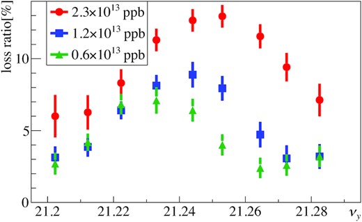
Intensity dependence of the beam losses with the present arc optics calculated by the SCTR simulations. The beam intensities were 2.3 × 10¹³ ppb (red), 1.2 × 10¹³ ppb (blue), and 0.6 × 10¹³ ppb (green). The other conditions were as listed in Table 6.
6. Verification of compensation by frequency analyses
The third set of experiments for the verification of the resonance compensation were Fourier analyses of the turn-by-turn positions of the beams. Fourier analysis is often used to obtain the tune of the optics. If the beam is affected by a resonance, the spectral line driven by the resonance can also be observed [38,39]. We compared the results of Fourier analyses for the present arc optics and for the new arc optics.
Relationships between resonances and spectral lines derived from the normal and skew quadrupole magnetic fields (p + q = 2) and the normal and skew sextupole magnetic fields (p + q = 3). The numbers in brackets in the spectral lines columns are the frequencies fu at a tune of (νx, νy) = (21.44, 21.24).
| Potential | jkml | Resonance | Horizontal spectral line fx | Vertical spectral line fy |
|---|---|---|---|---|
| x2 | 2000 | 2νx = n | −νx (0.44) | |
| y2 | 0020 | 2νy = n | −νy (0.24) | |
| xy | 1010 | νx + νy = n | −νy (0.24) | −νx (0.44) |
| 1001 | νx − νy = n | νy (0.24) | ||
| 0110 | −νx + νy = n | νx (0.44) | ||
| x3 | 3000 | 3νx = n | −2νx (0.12) | |
| 2100 | νx = n | |||
| 1200 | −νx = n | 2νx (0.12) | ||
| xy2 | 1020 | νx + 2νy = n | −2νy (0.48) | −νx − νy (0.32) |
| 1011 | νx = n | −νx + νy (0.20) | ||
| 1002 | νx − 2νy = n | 2νy (0.48) | ||
| 0120 | −νx + 2νy = n | νx − νy (0.20) | ||
| 0111 | −νx = n | νx + νy(0.32) | ||
| y3 | 0030 | 3νy = n | −2νy (0.48) | |
| 0021 | νy = n | |||
| 0012 | −νy = n | 2νy(0.48) | ||
| x2y | 2010 | 2νx + νy = n | −νx − νy (0.32) | −2νx (0.12) |
| 2001 | 2νx − νy = n | −νx + νy (0.20) | ||
| 1110 | νy = n | νx − νy (0.20) | ||
| 1101 | −νy = n | νx + νy (0.32) | 2νy (0.48) | |
| 0210 | −2νx + νy = n | 2νx (0.12) |
6.1. Simulation approach
First, the spectra of the resonances were analyzed using SCTR simulations. The tune was set at (νx, νy) = (21.44, 21.24) to observe the spectrum of the νx − 2νy = −21 resonance. At this tune, the spectra of the νx − 2νy = −21 resonance appear at (fx, fy) = (0.48, 0.20) in the units of the tune. The on-resonance condition was avoided because the spectra of the νx − 2νy = −21 resonance and the spectra of the tune would appear at the same frequencies.
The beams were injected with dipole errors in both the horizontal and vertical planes. The turn-by-turn transverse beam positions were acquired. Fourier amplitudes were calculated using numerical analysis of fundamental frequency (NAFF) [40] with Hanning windows. The number of turns used for the analyses was 512. The simulations were performed with both the present and new arc optics. For each, two kinds of simulation were conducted: one excluding the imperfections of the magnets, and another including these effects. The spectra appearing in the simulations without errors correspond to the structure resonances. On the other hand, all possible spectra appeared in the simulations with errors. The conditions used in the simulations are listed in Table 8.
Conditions of the simulations and the experiments for the Fourier spectral analyses.
| Number of bunches | 1 |
| Beam energy | 3 GeV |
| Tune (νx, νy) | (21.44, 21.24) |
| Chromaticity (ξx, ξy) | (−3, −3) |
| Beam intensity | 1.6 × 10¹² ppb |
| Initial transverse distribution | Gaussian |
| Initial emittance (εrms, x, εrms, y) | (1.0π, 1.0π) mm mrad |
| Initial longitudinal distribution | Parabola |
| Initial bunching factor Bf | 0.17 |
| Initial momentum spread σδ | 0.0013 |
| Number of macro particles | 200 000 |
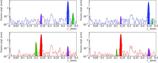
The images on the left of Fig. 16 show the results of the simulations using the present arc optics. In both the horizontal and vertical planes, the largest peaks corresponded to the tunes fx = 0.44 in the horizontal plane and fy = 0.24 in the vertical plane. The second largest peak in the horizontal plane appeared at fx = 0.48. This matched the frequency where the νx − 2νy = −21 resonance should appear. In the vertical plane, the second largest peak appeared at fy = 0.20. This also matched the frequency of the spectrum of the νx − 2νy = −21 resonance.

Horizontal (upper panels) and vertical (lower panels) Fourier spectral lines obtained from the simulation using the present (left) and new (right) arc optics. The horizontal axes represent the frequency with the units of the tune. The sky blue and orange areas show the results without the imperfections of the magnets, whereas the blue and red areas show those with errors.
As can be seen in Table 7, the spectrum at fx = 0.48 in the horizontal plane can be induced by the resonances νx + 2νy = n (jkml = 1020) and νx − 2νy = n (jkml = 1002). A candidate for the former is νx + 2νy = 63. However, it is too far from the working point. Thus, the peak at fx = 0.48 was excited by the νx − 2νy = −21 resonance. The vertical peak fy = 0.20 can be excited by the resonances νx = n (jkml = 1011) and νx − 2νy = n (jkml = 0120). A candidate for the former is νx = 21, but this resonance is too far as well. Consequently, it can be verified that the peak at fy = 0.20 was excited by the νx − 2νy = −21 resonance.
The images on the right of Fig. 16 show the results of the simulations using the new arc optics. Comparing the results with those of the present arc optics, it is obvious that the peaks at fx = 0.48 in the horizontal plane and fy = 0.20 in the vertical plane disappeared in the simulations without errors. This clearly shows that the νx − 2νy = −21 resonance was compensated in the new arc optics. In the results including errors, there were small peaks at fx = 0.48 and fy = 0.20 even in the new arc optics. This was because the νx − 2νy = −21 resonance was excited by the effects of magnet imperfections. The νx − 2νy = −21 resonance affected the beam as a nonstructure resonance. However, the peak height was still smaller than in the present arc optics. This is the difference between the structure and nonstructure resonance.
Let us discuss another peak. In the horizontal results, peaks appeared at fx = 0.24, only in the simulations with errors, for both the present and new arc optics. Since the spectra did not appear in the simulation without errors, the peak was due to the magnet imperfections. Based on Table 7, the possible sources are the resonances νx + νy = n and νx − νy = n. Considering the distance from the working point, the corresponding resonance is νx − νy = 0. The main source is the skew quadrupole magnetic field due to the rotational errors of the quadrupole magnets. Although it was not implemented in the simulations, the rotations of the BPMs can cause the spectra in the experiments. Since the BPM rotation is 0.96 ± 3.3 mrad in the MR [31], the horizontal peaks can appear in the vertical plane with a factor of 0.004 and vice versa.
According to the tables, the vertical peak due to the νx − νy = 0 resonance must appear at fy = 0.44. In fact, clear vertical peaks can be seen at fy = 0.44 in both the present and new arc optics, including errors. Similarly, the vertical peak fy = 0.44 is derived from the skew quadrupole magnetic field due to the rotational errors of the quadrupole magnets.
6.2. Experiments
The resonant spectra were also observed in experiments. The beams were intentionally injected with dipole errors in both the horizontal and vertical planes. The turn-by-turn transverse beam positions were acquired by the BPMs. The data where the betatron function was high were used for the analyses to obtain clear signals. The first 256 turns were used for the analyses. Though the maximum turn number of the data was approximately 2300, the spectra obtained by 256 or 512 turns were clearer than those obtained by 128 or 1024 turns because the dipole oscillations were damped. The set tune was (νx, νy) = (21.44, 21.24), which was the same as for the simulations. The spectra of the present and new arc optics were compared. The conditions used in the experiments were the same as in the simulation, and are listed in Table 8.
The images on the left side of Fig. 17 show the measured Fourier spectra with the present arc optics. The largest peaks, shown in blue (horizontal) and red (vertical), corresponded to the tunes. In the data, the tune was |$(f_x, f_y) = (0.436\, 736, 0.237\, 540)$|. The frequencies of the second highest peaks, shown in green, were |$(f_x, f_y) = (0.474\, 752, 0.199\, 253)$|. This matched (2νy, νx − νy) with an accuracy of 0.0003. Thus, the green peaks show the effects of the νx − 2νy = −21 resonance.
Horizontal (upper panel) and vertical (lower panel) Fourier spectral lines in the present (left) and new (right) arc optics, based on the measurements. The horizontal axes show the frequencies in the units of the tunes.
The spectra derived from the differential resonance νx − νy = 0 were also observed, and are colored violet. The peak position was |$(f_x, f_y) = (0.237\, 595,0.436\, 287)$|, which matched (νy, νx) with an accuracy of 0.0004.
The images on the right of Fig. 17 show the results with the new arc optics. The highest peaks, colored blue (horizontal) and red (vertical), represent the tunes. The positions of the peaks were |$(f_x, f_y) = (0.443\, 970, 0.237\, 501)$|. If there had been effects of the νx − 2νy = −21 resonance, resonant spectra would appear at (fx, fy) = (2νy, νx − νy). The nearest peaks are colored green in the right images of Fig. 17. The positions of the peaks were |$(f_x, f_y) = (0.470\, 968, 0.206\, 084)$|. Though the vertical peak position matched νx − νy with an accuracy of 0.0004, the horizontal peak position differed from 2νy by 0.004. This indicates that the horizontal peak around fx = 0.47 might be one of the noise peaks. In fact, its height was nearly at the noise level. The true horizontal peak was so small that it was hidden by other noise. Both the horizontal and vertical peak heights for the new arc optics were smaller than those for the present arc optics. Compared to the peaks of the tunes, the heights of the peaks of the νx − 2νy = −21 resonance were |$(x,y) = (3.26\%, 10.14\%)$| for the present arc optics. Meanwhile, the peak heights of the resonance were |$(x,y) = (0.95\%, 1.35\%)$| for the new arc optics. By using the new arc optics, the peaks of the νx − 2νy = −21 resonance were reduced to |$0.95\%/3.26\% = 29\%$| for the horizontal plane and |$1.35\%/10.14\% = 13\%$| for the vertical plane. The horizontal peak for the new arc optics could be smaller because the measured peak might be noise. These results clearly show that the νx − 2νy = −21 resonance was successfully weakened.
7. Conclusions
In this paper, a new method to compensate for the strength of the sextupole-driven third-order structure resonance was proposed, verified by simulations, and demonstrated in beam experiments at the J-PARC MR. New optics have been developed that make use of the MR synchrotron symmetry and properly adjust the vertical phase advance in the arc section Δψarc, y to cancel the resonance.
The compensation was verified by aperture survey simulations. It was demonstrated that the third-order structure resonance νx − 2νy = −21 (and the νx + 2νy = 63 resonance) were clearly compensated.
The compensation was also verified via three measurements. First, transverse couplings were measured. The beams were set on the νx − 2νy = −21 resonance and injected with dipole errors only in the horizontal plane. The turn-by-turn beam positions were measured to observe the propagation of the dipole oscillations from the horizontal to the vertical plane. The transverse beam couplings were observed only in the present arc optics. The measurements showed that the νx − 2νy = −21 resonance was well compensated in the new arc optics. The coupling measured in the present arc optics was analyzed. It was shown that the value Jc = 2Jx + Jy was preserved in a short time range. This verified that the coupling was caused by the νx − 2νy = −21 resonance.
Second, beam loss comparison was used to verify the compensation. The tune was scanned across the νx − 2νy = −21 resonance in both optics. The beam loss was clearly reduced in the new arc optics. This showed that the νx − 2νy = −21 resonance was successfully weakened. The results were well reproduced using SCTR. The peak tune was shifted from the on-resonance condition in both experiment and simulation. Since the shift became smaller when the beam intensity became weaker in the simulation, it was confirmed that the shift was due to space charge detuning.
Third, Fourier analyses were used to verify the compensation. The tune was set near the νx − 2νy = −21 resonance, and the Fourier spectra of the resonance were measured. The clear spectra of the resonance were measured in the present arc optics. Using the new arc optics, the spectra of the resonance were significantly suppressed. This showed that the νx − 2νy = −21 resonance was well compensated.
ACKNOWLEDGEMENTS
We would like to express our deepest gratitude to the power supply group in the MR for creating the various kinds of magnet patterns. We would like to give a special thanks to K. Ohmi for the implementation of SCTR. We are grateful to the monitor group in the MR for setting up the devices, such as BPMs, DCCT, Residual Gas Ionization Profile Monitor, and intra-bunch feedback systems. We appreciate the kind cooperation of the members of the RF, 3-50BT, injection/extraction, control, and vacuum groups in the MR.
Appendix A. Tuning arc section
The most important part of the optics tuning is to gain accurate control of the phase advance in the arc section. In the MR, there are four kinds of quadrupole magnets in the arc sections which change the phase advance in the arc section.
The phase constant φu was obtained via Fourier analysis (NAFF). The data for the first 512 turns were used in these analyses. We defined φu as the Fourier phase term at the peak frequency.
The phase advance of the new optics in one arc section is (Δψarc, x, Δψarc, y) = 2π(6, 5.5). First, the phase advances were measured with the setting values. The horizontal phase advance Δψarc, x was well adjusted, but the vertical phase advance Δψarc, y had a systematic error. This indicated that the calibrations of the quadrupole magnets in the arc sections around the new settings were not perfect. Therefore, the vertical phase advance Δψarc, y was calibrated.
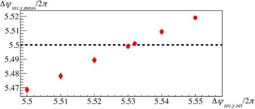
Calibration of the vertical phase advance Δψarc, y for the new arc optics. The horizontal axis shows the setting of the vertical phase advance Δψarc, y from the SAD, and the vertical axis shows that from the experiment. The error bars show the root mean squares of the data.
Appendix B. Optical measurements
Before the experiments for the verification of the compensation, the tune, the betatron functions, and the dispersions were measured to verify the beam optics. In this section the results for the new arc optics are presented.
The betatron functions were obtained using the phase advances between three adjacent BPMs [42]. The phase advances were measured by using beams with dipole errors at the beam injection. All the dipole oscillations at the BPMs were analyzed via NAFF. The first 128 turns of data were used for the analysis. The results of the betatron functions are shown in Fig. B1.
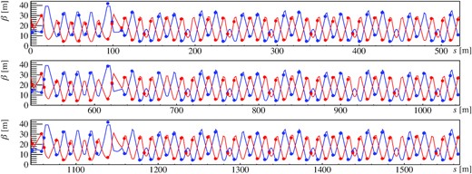
Betatron function of the new arc optics. The lines show the setting betatron functions obtained from the SAD, and the circles denote the measured ones. The blue line and circles represent the horizontal betatron functions, and the red ones represent the vertical betatron functions.
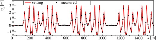
Dispersion function of the new arc optics. The results of the experiments are denoted as black circles. The red line shows the setting dispersion function calculated by the SAD.
Footnotes
The definition of the space charge tune shift is [28] |$\Delta \nu _{\mathrm{SC}} = -F_{\mathrm{B}} N_{\mathrm{B}} r_0 /2\pi \varepsilon _{\mathrm{N}} \beta _{\mathrm{rel}} \gamma _{\mathrm{rel}}^2$|, where |$F_{\mathrm{B}} = C/\sqrt{2\pi } \sigma _l$|, NB is the number of protons per bunch, r0 is the classical radius of a proton, εN = βrelγrel4εrms, (βrel, γrel) are Lorentz factors, C is the circumference, σl is the bunch length, and εrms is the transverse rms emittance.
References
K. Nakamura and
