


Abstract
The small binding energy of the hypertriton leads to predictions of the non-existence of bound hypernuclei for isotriplet three-body systems such as nnΛ. However, invariant mass spectroscopy at GSI has reported events that may be interpreted as the bound nnΛ state. The nnΛ state was sought by missing-mass spectroscopy via the (e, e′K+) reaction at Jefferson Lab’s experimental Hall A. The present experiment has higher sensitivity to the nnΛ-state investigation in terms of better precision by a factor of about three. The analysis shown in this article focuses on the derivation of the reaction cross-section for the 3H(γ*, K+)X reaction. Events that were detected in an acceptance, where a Monte Carlo simulation could reproduce the data well (|$|\delta p/p| \lt 4\%$|), were analyzed to minimize the systematic uncertainty. No significant structures were observed with the acceptance cuts, and the upper limits of the production cross-section of the nnΛ state were obtained to be 21 and |$31 \, \rm {nb} \, \rm {sr}^{-1}$| at the |$90\%$| confidence level when theoretical predictions of (−BΛ, Γ) = (0.25, 0.8) MeV and (0.55, 4.7) MeV, respectively, were assumed. The cross-section result provides valuable information for examining the existence of nnΛ.
1. Introduction
An extension of nuclear (NN) interaction to baryon (BB) interaction with strangeness degrees of freedom in the SU(3) flavor symmetry is one of the major subjects of study in nuclear physics. Studies of hypernuclei which have at least one strange quark have played an important role in the understanding of the hyperon–nucleon (YN) interaction.
Hypertriton, which is composed of a neutron, a proton, and a Λ, is known as the simplest bound hypernuclear system. The hypertriton binding energy was measured to be |$130\pm 50\, \rm {keV}$| by an emulsion experiment [1]. The small binding energy in the isospin singlet (T = 0), three-body (A = 3) hypernuclear system suggests that no bound systems exist for isotriplet (T = 1), A = 3 hypernuclei such as ppΛ and nnΛ. However, events that may be interpreted as the bound state of nnΛ were observed in t + π− invariant mass spectroscopy at GSI [2]. The measured binding energy and width were |$-B_\Lambda =0.5\pm 1.1\pm 2.2$| MeV and Γ = 5.4 ± 1.4 MeV, respectively, for a vertex cut of |$-2 \, \mathrm{cm} \lt Z \lt 30$| cm.
As well as the early study in Ref. [3], theoretical calculations with recently developed interaction models have been unable to reproduce a bound state such as was observed at GSI. For example, Faddeev [4–9] and variational methods [10] do not support the occurrence of the bound state. Although a calculation based on pion-less effective field theory (|$\backslash \!\!\!\pi$|-EFT) suggested the existence of the bound state as an Effimov state, there were no quantitative discussions [11].
On the other hand, the existence of a resonant state of nnΛ was predicted by some theories. By using the two-body S-wave potential in the framework of three-body Jost functions, Ref. [12] suggested the existence of the resonant state, which according to their estimate had a decay width of approximately a few MeV. Reference [6] predicted a broader state, while Ref. [8] obtained a narrower state of less than |$1\, \rm {MeV}$| using the Faddeev calculation method. The |$\backslash \!\!\!\pi$|-EFT calculation with specific interaction models also supported the existence of the broader state [13,14]. A prediction in Ref. [5] suggested that even though a resonant state of nnΛ does not exist with the standard strength of the Λn interaction, the existence of the resonant state may become possible with a Λn interaction that is more attractive by about |$5\%$|.
The nnΛ state needs to be experimentally confirmed. In emulsion experiments, neutron-rich systems such as nnΛ are relatively hard to uniquely identify, and indeed, no signals of the nnΛ system were found. Conventional counting experiments that use the (π+, K+) or the (K−, π−) reactions never have an available target (nnn) to produce such a state because these reactions convert a neutron into a Λ. Invariant mass spectroscopy with heavy ion beams or collisions can search for the signal of nnΛ, as previously reported [2]. Invariant mass spectroscopy of hypernuclei measures weak-decayed particles like the emulsion experiments. Therefore, both invariant mass spectroscopy and emulsion experiments have much less sensitivity for the detection of the resonant state, which tends to decay in the presence of the strong interaction.
Missing-mass spectroscopy is a powerful tool for investigating the nnΛ state because it allows measurement of both the bound and resonant states. Missing-mass spectroscopy of Λ hypernuclei with the (e, e′K+) reaction was developed at Jefferson Lab (JLab), and high-resolution hypernuclear data were successfully published [15–19]. However, a tritium target, which requires strict regulations to be followed concerning safety issues, is necessary for (e, e′K+)-reaction spectroscopy, because a proton gets converted into a Λ in the reaction. The use of a tritium target was realized in 2017, thanks to the great efforts of the JLab Tritium Target Group [20], which gave us a chance to perform an experiment to investigate the nnΛ state at JLab’s experimental Hall A (JLab E12-17-003 Experiment).
We performed the experiment with the 3H(e, e′K+)X reaction in October–November, 2018. Both arms of the high-resolution spectrometers (HRS-L and HRS-R) [21] in JLab Hall A were used for analysis of the momentum vectors of e′ and K+ at reaction points to reconstruct the missing mass. The data were successfully taken, and analysis that focused on the cross-section derivation was performed. Strict event-selection conditions, particularly for the momentum selection, were set to minimize the systematic uncertainty of the result; the conditions were stricter than those of other analyses, such as (i) a spectrum analysis with loosened cuts for peak search and (ii) a distribution analysis of the quasi-free Λ production for a study of Λn final state interaction (FSI). These other analyses will be discussed elsewhere.
The present article contains the following details. Our experimental kinematics for the (e, e′K+) reaction, the electron beam provided by the Continuous Electron Beam Accelerator Facility (CEBAF) at JLab, and the experimental apparatus are discussed in Sect. 2. Section 3 describes the data analysis. Section 4 discusses the results, followed by a conclusion in Sect. 5.
2. Experiment
The missing-mass spectroscopy measurements using the (e, e′K+) reaction were conducted at JLab Hall A. In this experiment, 4.32 GeV/c electron beams were impinged on the tritium target. The scattered electrons and the K+s produced were measured using HRS-L and HRS-R, respectively [21].
2.1 Kinematics
A schematic of the (e, e′K+) reaction is shown in Fig. 1. The one-photon exchange approximation, which assumes that a virtual photon mediates the reaction, is generally used in the electro-production.
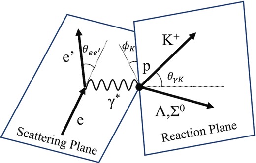
Schematic of the (e, e′K+) reaction. A virtual photon reacts with a proton to produce the Λ (or Σ0) and a K+.
The HRSs were at the scattering angles of |$\theta _{ee^{\prime }} = \theta _{eK} = 13.2^{\circ }$| in the laboratory frame and had central momenta of 2.218 GeV/c and 1.823 GeV/c for e′ and K, respectively, for the physics runs (physics mode: |$\rm {M_{phys.}}$|). The |$\rm {M_{phys.}}$| mode had sufficient acceptance to cover the region where the nnΛ state may exist. A proton (hydrogen) target was also used in the |$\rm {M_{phys.}}$| mode to measure the p(e, e′K+)Λ reaction for energy calibration, as shown in Sect. 3.1. For the purpose of calibration, data with a different momentum setting for the e′ (calibration mode: Mcalib.) was used. In the Mcalib. mode, the e′ central momentum was decreased to |$2.100\, \rm {GeV/{\it c}}$|, which allowed simultaneous measurements of Λ and Σ0 from the proton target, whereas the nnΛ production became almost out of the acceptance (Fig. 2). It may be noted that we did not decrease the K+ momentum to avoid the low survival probability of the K+. The kinematical parameters are summarized in Table 1.
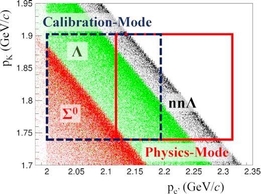
Correlations between the momenta of e′ and K+ for the p(e, e′K+)Λ (green dots), p(e, e′K+)Σ0 (red dots), and 3H(e, e′K+)nnΛ (black dots) reactions in a Monte Carlo simulation. The boxes with solid and dashed lines represent the acceptances for the physics and the calibration modes (Mphys. and Mcalib.), respectively.
Major parameters for the present experiment. The p(e, e′K+)Λ reaction was assumed for the calculations of |$\sqrt{s}$| and the momentum transfer q.
| Calibration mode | Physics mode | ||
|---|---|---|---|
| (|$\rm {M_{calib.}}$|) | (|$\rm {M_{phys.}}$|) | ||
| Reaction | p(e, e′K+)Λ/Σ0 | p(e, e′K+)Λ | |
| 3H(e, e′K+)nnΛ | |||
| |$p_{e^{\prime }}^{\rm {cent.}}$||$(\rm {GeV}/{\it c})$| | 2.100 | 2.218 | |
| |$p_K^{\rm {cent.}}$||$(\rm {GeV/{\it c}})$| | 1.823 | ||
| Q2|$(\rm {GeV/{\it c}})^2$| | 0.479 | 0.505 | |
| θeγ(deg) | 11.9 | 13.2 | |
| q|$(\rm {GeV/{\it c}})$| | 0.497 | 0.389 | |
| |$\sqrt{s}$||$(\rm {GeV})$| | 2.13 | 2.07 | |
| ϵ | 0.769 | 0.794 | |
| ϵL | 0.075 | 0.092 | |
2.2 Electron beam
We used 4.32 |$\rm {GeV/{\it c}}$| electron beams provided by CEBAF at JLab. The typical beam current on the target was |$22.5 \, \mu$|A with a raster size of |$2\times 2 \, \rm {mm^2}$|. The spread and drift of the beam energy were well controlled and monitored during the experiment [25]. The total energy uncertainty was approximately ΔE/E ≲ 1 × 10⁻⁴ in full width at half maximum (FWHM). The beam current was measured by the Parametric Current Transformer system and the beam current monitor, with an uncertainty of approximately |$1.0\%$| [20,26,27]. The total beam charges on the tritium and hydrogen targets were 16.9 C and |$4.7\, \rm {C}$|, respectively, for the data used in the present analysis.
2.3 Overview of experimental apparatus
The tritium gas was enclosed in a target cell made with the aluminum alloy Al-7075. The target-cell length along the beam direction was |$25\, \rm {cm}$|, and the areal density was |$84.8\pm 0.8\, \rm {mg} \, \mathrm{cm}^{-2}$| for the gas. The target cell was cooled down to |$40\, \rm {K}$| during beam operation, resulting in a gas pressure of 0.3 MPa. Hydrogen gas was used for energy calibration, as shown in Sect. 3.1. The target cell for the hydrogen gas was the same shape as for the tritium target. The areal density for the hydrogen target was |$70.8\pm 0.4\, \rm {mg} \, \mathrm{cm}^{-2}$|. The gas density was reduced during the beam irradiation due to a local heat deposit along the beam path. This reduction was evaluated as a function of the beam intensity, and it was found that the tritium gas density was reduced by |$10\%$| at a beam intensity of |$22.5\, \mu$|A [20]. It is noted that tritium decays to |$^3\rm {{He}}$| with a lifetime of 12.32 yr [28]. The reduction effect of the tritium nuclei due to this decay was taken into account when the cross-section was calculated, as shown in Sect. 4.1.
HRS-L and HRS-R were used for the detection of e′ and K+, respectively. Each spectrometer is composed of three quadrupole and one dipole magnets (QQDQ), and their optical features are basically identical. The path length from the target to the focal plane is |$23.4\, \rm {m}$|. The designed momentum resolution is Δp/p = 1 × 10⁻⁴ (FWHM). However, the momentum resolution was limited because of the materials, particularly for the target cell. The expected energy resolution in the resulting spectrum for which the effects of the target cell material etc. were taken into account is described in Sect. 4.2.
The configurations of the spectrometers were similar to each other. Each spectrometer had vertical drift chambers (VDC) for particle tracking [29] and plastic scintillation detectors (S0 and S2) for time-of-flight measurement, which were installed in this order from upstream. Cherenkov detectors were installed between S0 and S2 for particle identification [30]. The plastic scintillation detectors were used for a data-taking trigger with the following condition: |$\rm {(S0\otimes S2)_L \otimes (S0\otimes S2)_R}$|, where the subscripts L and R represent the hit conditions for HRS-L and HRS-R, respectively. The Cherenkov detectors were not used for the main trigger but were used in offline analyses. A |$\rm {CO_2}$|-gas Cherenkov detector was used to remove π−s in HRS-L. In HRS-R, on the other hand, two aerogel Cherenkov detectors (AC1 and AC2; refractive indices of n = 1.015 and 1.055, respectively) were used to remove the background π+s and protons, as shown in Sect. 3.3.
2.4 Summary of measurements
We performed missing-mass spectroscopy with the |${^3\rm {H}}(e,e^{\prime }K^+)\textrm {X}$| reaction at JLab Hall A. Two existing spectrometers (HRSs) were used to detect e′ and K+. H(e, e′K+)Λ and H(e, e′K+)Σ0 reactions were also measured for calibration. The experimental data were taken in October–November, 2018.
3. Analysis
3.1 Missing-mass reconstruction
Multi-carbon foils were used as targets instead of the gas target for the zT calibration. Ten foils were placed at a distance of |$2.5\, {\rm {cm}}$| from each other except for the second and third foils, between which the distance was set to |$5\, {\rm {cm}}$|. Each foil had an areal density of approximately |$45\, {\rm {mg} \, \mathrm{cm}^{-2}}$|. Figure 3 shows a zT distribution reconstructed by HRS-L. Separated peaks from the carbon foils are clearly seen. The Cz parameters in Eq. (11) for both HRSs were optimized to reproduce the foil positions using the MINUIT algorithm [31,32].

Reconstructed zT for data with multi-carbon foils using HRS-L.
The parameters for the angles, |$C_{x^{\prime }}$| and |$C_{y^{\prime }}$| in Eqs. (8) and (9), were optimized using the calibration data with sieve slits. The sieve slits (SS) were made of 2.54 cm-thick tungsten plate with holes through which the particles could be detected in the spectrometers [33]. Dedicated data were taken with the SS attached in front of the first quadrupole magnet for each HRS. Figure 4 shows a particle-position image in HRS-L that was reconstructed using the particle angles and the distance between target and SS. The angle parameters in Eqs. (8) and (9) were optimized to reproduce the hole patterns that were expected. It may be noted that the holes had diameters of 4 mm and 6 mm.
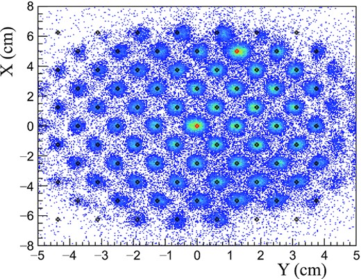
xy image at the sieve slit for the HRS-L sieve slit data. The image was reconstructed using the reconstructed angles and distance between target and SS. The markers represent the hole positions that we expected.
The momentum parameters, Cp in Eq. (10), were optimized using data obtained from the hydrogen target. Λ and Σ0 production events were detected in |$\rm {M_{calib.}}$|, whereas only Λ production events were detected in |$\rm {M_{phys.}}$|. The missing mass was reconstructed to observe the Λ and Σ0 peaks. The Cp were optimized to make their peak means consistent with the Particle Data Group (PDG) masses [34]. The missing-mass resolution after momentum calibration was found to be |$\sigma = 1.3\pm 0.1\, \rm {MeV/}{{\it c}}^2$| when a fit was performed with a Gaussian function over a range of |MX − MΛ| < 2 MeV/c2.
The Λ binding energy is defined as follows: |$B_\Lambda = {\rm M_{core}} + {\rm M_\Lambda } - {\rm {M}}_X$|. In the present analysis we took Mcore = 2Mn, where Mn is the mass of a neutron. The masses of the Λ and the neutron MΛ, n were taken from Ref. [34]. The nuclear masses of the hydrogen and tritium targets, |$\rm {M_t}$| used in Eq. (7), were taken from Refs. [34,35], respectively.
3.2 Event selection for gas target
The production position along the beam axis zT was independently reconstructed in HRS-L and HRS-R. Event selection by the zT difference between the HRS-L and HRS-R was applied as |$\big |z_{\rm {T}}^{\rm {diff}}\big | = \big |z_{\rm {T}}^{\rm {L}}-z_{\rm {T}}^{\rm {R}}\big | \lt 2$| cm. Figure 5 shows the average of |$z_{\rm {T}}^{\rm {L}}$| and |$z_{\rm {T}}^{\rm {R}}$|: |$z_{\rm {T}}^{\rm {mean}} = \big (z_{\rm {T}}^{\rm {L}}+z_{\rm {T}}^{\rm {R}}\big )/2$|. The individual resolutions of |$\sigma \big (z_{\rm {T}}^{\rm {L}}\big )=0.53$| cm and |$\sigma \big (z_{\rm {T}}^{\rm {R}}\big )=0.50$| cm were improved to |$\sigma \big (z_{\rm {T}}^{\rm {mean}}\big )=0.38$| cm by considering the average. The peaks at −12.5 cm and +12.5 cm correspond to events from the target cell. Therefore, events for |$\big |z_{\rm {T}}^{\rm {mean}}\big | \lt 10$| cm were selected for the gas-target analysis. A fit was performed to estimate the amount of gas used for the analysis with the cut as shown in Fig. 5. Second-order polynomial functions convoluted by a Gaussian function f1 and two Gaussian functions f2 were used for the gas and the cell regions, respectively. Here, the widths of the Gaussian functions f1 and f2 were the same. As a result, |$71\%$| of the full amount of gas was used with the cuts of zdiff and zmean. The contamination from the target cell was estimated to be less than |$0.1\%$|, which is fairly small.
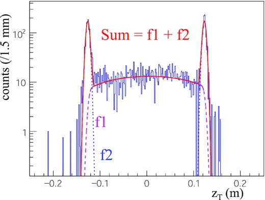
Distribution of |$z_{\rm {T}}^{\rm {mean}} = \big (z^L_{\rm {T}} + z^R_{\rm {T}}\big )/2$| for the data with the tritium target. A fit with seconnd-order polynomial functions convoluted by a Gaussian function (f1) and two Gaussian functions (f2) was performed for the gas and the target cell regions, respectively. It is noted that the width of the Gaussian function f1 is the same as that of f2.
3.3 Particle identification
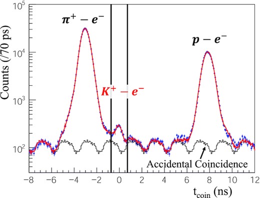
Distribution of coincidence time as defined in Eq. (12). The distribution of the accidental coincidence backgrounds was evaluated by collecting some accidental bunches. The fitting result is shown by the red solid line.
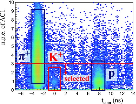
The number of photoelectrons in AC1 as a function of tcoin.
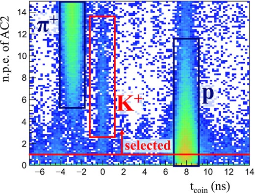
The number of photoelectrons in AC2 as a function of tcoin.
3.4 Monte Carlo simulation
A Monte Carlo (NC) simulation based on Geant4 [36–38] was coded and used to estimate the acceptance and other factors required for the cross-section analysis such as the decay and absorption factors of K+s in HRS-R (Sect. 3.6). In addition, MC simulation was used to estimate the momentum loss in materials such as the target, detectors, air, and so on (Sect. 3.5). In the MC simulations, the precise geometries were modelled.
A three-dimensional magnetic field map for the dipole magnet was calculated using Opera3D (TOSCA), and was incorporated into the MC simulator. In contrast, the magnetic fields for the quadrupole magnets were calculated by an empirical formula taken from Ref. [39]. The magnetic fields obtained by the calculation were not the same as those for the real experiment because of the arithmetic precision and an imperfection of the model. Therefore, we scanned the magnetic field strengths to find reasonable magnetic field settings that reproduced the experimental data. We scanned various combinations of magnets field strengths (QQDQ), comparing the distributions of momentum vectors at the production point and angle distributions of particles at the focal plane between the simulation and the real data. The effective strengths of the magnetic fields obtained by the scan were used for the MC simulation to estimate the acceptance and some correction factors, as shown in Sect. 3.6. The systematic error on the final result originating from the magnetic field settings (acceptances) are described in Sect. 4.3.
Elementary reaction data for Λ and Σ0 from the hydrogen target were used for validating the MC simulation and the event generator. Events were generated by the Geant4 MC simulation, and the missing-mass reconstruction was performed with the same analysis code as the real data analysis. The input parameters of the simulation were position and angular resolutions at the focal plane based on the VDC resolution [21]. The momentum vectors at the production points were calculated by the backward transfer matrices, as shown in Eqs. (8)–(10). Figure 9 shows the missing-mass spectrum obtained in the MC simulation compared with the experimental data. The simulation agrees well with the experimental data.
Missing-mass spectrum for the p(e, e′K+)Λ/Σ0 reaction with the momentum setting of Mcalib.. The data are shown by markers with statistical error bars, and the MC simulation spectra are shown by histograms.
3.5 Energy loss correction
Particles lose their energies in materials, and the energy losses need to be considered for the missing-mass reconstruction. The measurable quantity in our experiment was the momentum. Therefore, a correction for the momentum is a more practical option than the energy-loss correction used in the previous hypernuclear experiment [17]. The momentum-loss correction was applied event by event depending on y′ and |$z_{\rm T}^{\rm mean}$| for e′ and K+. The dependence on y′ and |$z_{\rm T}^{\rm mean}$| came from the shape of the target cell [20]. On the other hand, a fixed value correction was applied to the incident electron beam. The correction function was obtained from the MC simulation in which the precise geometry was modelled as described in Sect. 3.4.
3.6 Efficiencies
The efficiencies and correction factors needed for the cross-section calculation were evaluated, and are summarized in Table 2. The cross-section calculation with the acceptance of HRS-R (|$\Omega ^{\rm {HRS\textrm {-}R}}$|), the K+ decay factor, and the K+ absorption factor were applied event by event depending on the particle momenta. The other efficiencies and correction factors were applied as fixed values for all events.
Efficiencies and correction factors used for the cross-section calculation in Eq. (13).
| Item | Efficiency or correction factor | Regard |
|---|---|---|
| ϵtrack | 0.981 | Tracking efficiency estimated from the data analysis and a simple MC simulation. |
| ϵdecay | 0.15 at pcent. | K+ survival ratio against its decay estimated by Geant4 MC simulation. |
| ϵT | 0.986 | Survival ratio of the tritium gas against its decay with |$^3\rm {H}\rightarrow ^3\rm {He}+e^-+\bar{\nu }_e$|. |
| 1/ϵHe | 0.97 | Correction factor to correct the 3He contamination from the tritium decay. A ratio of quasi-free Λ production from 3H to that of 3He was assumed to be the same as for the (e, e′p) reaction [40]. |
| ϵDAQ | 0.95 | Efficiency of data acquisition system and trigger counters [41]. |
| ϵctime | 0.96 | Efficiency for the real coincidence selection by the coincidence time (Fig. 6). |
| ϵabsorp | 0.91 at pcent. | Survival ratio of K+ against its absorption in materials due to the K+N interaction. Estimated by the Geant4 MC simulation. |
| ϵdensity | 0.901 | Density reduction effect of the gas due to the heat by beam irradiation [20]. |
| ϵvertex | 0.71 | zdiff and zmean cuts shown in Sect. 3.2. |
| ϵPID | 0.91 | Survival ratio of signals after the particle identification by the gas and aerogel Cherenkov detectors. |
| 1/ϵπ | 0.98 | Correction factor to correct the π contamination. |
4. Results and discussions
4.1 Derivation of the differential cross-section
The differential cross-section for the 3H(γ*, K+) reaction as a function of |$-B_\Lambda$| is shown in Fig. 10. The distribution of the accidental coincidence between e′ and K+ is shown with an extremely small uncertainty. This distribution was evaluated by randomly combining e′ and K+ in the analysis (mixed event analysis) [42,43].
![Differential cross-section of the reaction 3H(e, e′K+)X as a function of $-B_\Lambda$. The distribution of the accidental coincidence events was obtained via mixed event analysis [42,43]. The error bars are statistical only.](https://oup.silverchair-cdn.com/oup/backfile/Content_public/Journal/ptep/2022/1/10.1093_ptep_ptab158/5/m_ptab158fig10.jpeg?Expires=1750211145&Signature=maSE79sNqv1oN3BekUpYzQ9KV3WOurj9VPqpYVd3rx2j7mYRerl4TqZVujwZC2wwwpShxKGHf-d9e--Vb5-p2RiZJaTtHPUPaC5i2OhoWPIvvwBbkccXsA-try~MdG~xaRw92nXJldaPBA3HhCVCfenJKX~Ey8PFD~0R2c6nF5P9hDLSM8TSIDy5m7dLWqHRTW4BCw-VVkOpa6Ye-0AULL9gypuWPZcRVZQBBxH26NYOY5tuUPa3hSyuJBvwhjN2-wiU5zu4TMcu9viay8FGGuPSUtKf9J4LWZlRJheyXXMhKZ-15h4IRvnMKAAVWs3GvY29Qh6eo1oYuRMY9buzWg__&Key-Pair-Id=APKAIE5G5CRDK6RD3PGA)
4.2 Energy resolution
The energy resolution was estimated from MC simulation (Sect. 3.4). The simulation considered the energy straggling and multiple scattering effects in the materials, as well as the optics of the spectrometers. As a result, the expected resolutions were found to be σ = 1.4 ± 0.1 MeV and 1.5 ± 0.2 MeV for Λ and nnΛ production, respectively. The errors on the expected resolutions come mainly from the variations of the possible magnetic field settings that could reproduce the data distributions of the momentum vectors at the production point and the angle distributions of the particles at the focal plane.
4.3 Systematic uncertainties
The systematic errors on the cross-section and the binding energy were estimated, and Table 3 shows the systematic uncertainties for the major efficiencies and the correction factors. The largest contribution to the cross-section uncertainty comes from the acceptance of the spectrometer system. The magnetic fields of the spectrometer magnets (QQDQ) in the MC simulation were changed and scanned so that the various particle distributions at the target and focal plane become consistent with those of the real data, as shown in Sect. 3.4. In the scan, several magnetic field settings that could reproduce the experimental data were found. We derived the differential cross-sections with the possible field settings that corresponded to the possible acceptances, and the difference was considered as the systematic error on the result. The variations of |$\Omega ^{\rm HRS\textrm {-}R}$| and Γint are |$\pm 7.6\%$| and |$\pm 8.5\%$|, respectively, due to the difference of the possible field settings. The error on the acceptance shown above was evaluated over the whole acceptance. The |$\Omega ^{\rm HRS\textrm {-}R}$| correction was applied event by event depending on the particle momentum in the present analysis. Therefore, a resultant error due to the |$\Omega ^{\rm HRS\textrm {-}R}$| uncertainty is affected by the momentum data distribution.
Relative errors for the efficiencies and correction factors that contributed to the uncertainty on the cross-section calculation in addition to the acceptance uncertainties.
| Item | Relative error |
|---|---|
| Δϵtrack | |$0.2\%$| |
| ΔϵT | |$0.3\%$| |
| ΔϵHe | |$0.7\%$| |
| ΔϵDAQ | |$0.1\%$| |
| Δϵctime | |$0.5\%$| |
| Δϵdensity | |$1.1\%$| |
| Δϵvertex | |$7.8\%$| |
| ΔϵPID | |$6.9\%$| |
| Δϵπ | |$1.8\%$| |
| ΔΓint | |$8.5\%$| |
| ΔNe | |$1.0\%$| |
| ΔNT | |$0.9\%$| |
| ΔNHYP | |$6.8\%$| |
| Single track selection | |$1.3\%$| |
| Total | |$15\%$| |
Major contributions to the systematic uncertainty on |$B_\Lambda$| were obtained from (i) the calibration method and (ii) the correction of momentum loss in materials, particularly for the target cell. The uncertainty that comes from the calibration method using Λ and Σ0 production was evaluated to be about |$\pm 0.1\, \rm {MeV}$| in the previous hypernuclear experiment [17], which was performed following the same method. We analyzed the p(e, e′K+)Λ peak from the tritium gas target, in which a small percentage of hydrogen contamination took place. It is noted that the hydrogen contamination made a broad peak at −BΛ ∼ +45 MeV in the spectrum of the 3H(e, e′K+)X reaction, and the uncertainty related to the hydrogen contamination does not affect the present analysis of the differential cross-section. We applied a missing-mass correction to make the Λ peak from the hydrogen contamination become consistent with the PDG mass [34]. This correction yielded an uncertainty of |$\Delta B_{\Lambda }^{\rm {A}} = \pm 0.3$| MeV, which is from the statistical uncertainty of the Λ peak arising from the hydrogen contamination in the tritium gas cell. The target cell thickness needed to be assumed in the MC simulation to obtain the momentum-loss correction values. However, the target cell was not uniform and had sample standard deviations of |$7.6\%$| and |$25\%$| for the tritium and hydrogen gas target cells, respectively. The deviations of the cell thickness caused the uncertainty of the particle momentum-loss corrections. This effect was evaluated to be |$\Delta B_{\Lambda }^{\rm {B}} = \pm 0.1$| MeV if the correction by the Λ peak from the H contamination in the tritium gas cell is performed with no uncertainties. Therefore, the systematic error that comes from the momentum-loss correction was found to be |$\sqrt{(\Delta B_{\Lambda }^{\rm {A}})^2 + (\Delta B_{\Lambda }^{\rm {B}})^2} = \pm 0.32$| MeV.
In total, the systematic error on |$B_\Lambda$| was evaluated to be |$\Delta B_{\Lambda }^{\rm {sys.}} = \pm 0.4\, \rm {MeV}$| for the present analysis.
4.4 Upper limit analysis and discussion
The nnΛ signal was searched for in a threshold region of −BΛ ranging from −20 MeV to 20 MeV. We performed the spectral fits assuming the distributions for QF Λ, accidental coincidence, and signal to analyze the differential cross-section. The spectral fits were carried out by unbinned maximum likelihood with the RooFit toolkit [44]. Background QF events start to rise at −BΛ = 0 MeV and monotonically increase as a function of |$-B_\Lambda$| in the threshold region. The QF distribution at the threshold region in particular is affected by the Λn FSI and becomes complicated. However, there are no theoretical predictions for the QF distribution with the FSI so far. Therefore, in the present analysis we assumed a linear function, which is the simplest assumption for the QF background. A distribution function for the accidental coincidence was obtained by a fit with the fourth-order polynoamial function for the accidental coincidence distribution that was obtained by the mixed event analysis (Sect. 4.1).
The experimental peak has a long tail, mainly due to the external and internal radiation [45], as shown in Fig. 9. A response function for the signal was obtained by MC simulation. In addition to the response function, which includes the experimental resolution and the tail component, the decay width Γ of the nnΛ state needs to be considered. Here, we convoluted a Breit–Wigner function with the decay width Γ into the experimental response function to make a template function for the signal. There is a slight difference between the data and MC simulation for the tail component in the Λ production spectrum shown in Fig. 9, and there may be a similar difference in the tail component for the nnΛ production. The error that may come from the difference in the tail shape was evaluated by a simple test. In the test, the tail shape of the MC simulation, which was adjusted to the data for Λ production, was adopted as the response function for the nnΛ production when the spectral fit was performed. As a result, the systematic error on the cross-section originating from the tail shape uncertainty was evaluated to be |$\Delta N_{\rm HYP} = \pm 6.8\%$|.
The top part of Fig. 11 shows the fitting result with assumptions of |$(-B_\Lambda , \Gamma ) = (0.25,0.8)$| MeV and |$(0.55,4.7)\, \rm {MeV}$|, which are theoretical predictions obtained from Refs. [8,12], respectively. The differential cross-sections were obtained to be |$11.2\pm 4.8({\rm {stat.}})^{+4.1}_{-2.1}({\rm sys.})$| nb sr−1 and |$18.1\pm 6.8({\rm {stat.}})^{+4.2}_{-2.9}({\rm sys.})$| nb sr−1 for the assumptions of |$(-B_\Lambda ,\Gamma ) = (0.25, 0.8)$| MeV and (0.55,4.7) MeV, respectively. Given the decay widths, the differential cross-sections as a function of the assumed peak position are shown in the bottom part of Fig. 11. The systematic errors are represented by the selection symbols. There seem to be some excesses in the range from −5 MeV to 5 MeV for both decay width assumptions: one is narrow and the other is wide. However, the excesses do not have a statistical significance of more than |$3 \, \sigma$|. It is noted that the differential cross-section becomes negative for the region about −BΛ > 10 MeV. This is because of a larger gradient of the linear function for QF, which was led by some events around −BΛ = 0 MeV. The larger gradient of the linear function alone caused an overestimation at −BΛ > 10–12 MeV, leading to a negative amplitude of the signal function. In addition, the fraction of the area outside the fit region (−BΛ > 20 MeV) for the tail component of the signal function increases as the assumed peak position becomes larger. Therefore, the fit results for −BΛ > 10–12 MeV have another systematic error in addition to the systematic errors that we considered in the present analysis.
![The differential cross-section as a function of $-B_\Lambda$ (MeV). Spectral fits were done by assuming $(-B_\Lambda , \Gamma )=(0.25,0.8)$ MeV and (0.55,4.7) MeV respectively, which are predictions adopted from Refs. [8,12]. Each panel shows the differential cross-section of exceeded events over the assumed QF distribution as a function of an assumed peak center.](https://oup.silverchair-cdn.com/oup/backfile/Content_public/Journal/ptep/2022/1/10.1093_ptep_ptab158/5/m_ptab158fig11.jpeg?Expires=1750211145&Signature=a-4InNLFRQUqBILI2YG5rbJL6cjL~ph2sAZOPpQDQ8zV0lWTakSljLulRo7krovwB8VHwKzwDUBMKTLO3supJqvw3JlQXgZQq1cEHtKuOExKJzLt5FHzQf4EfjnaOPhVshNsBRToLbwRs6C6KUbbfvJG3BDHRxL0bl~DCKw23b8VBEkxVlbg8jNmYYTkqENQapEotz4336bsP4pF8QXbkaWRojN3u-C1vlUJT9hHobgLPXPtNzYR1zPGRhYDbo4P6NSQd~WydjiunlF57RDrSA33kwEH8QllHvqMoSgK0oyprCYN2EVUtkMbGidk1o38UeK8lBjfi69ZLbVwCTEq0Q__&Key-Pair-Id=APKAIE5G5CRDK6RD3PGA)
The differential cross-section as a function of |$-B_\Lambda$| (MeV). Spectral fits were done by assuming |$(-B_\Lambda , \Gamma )=(0.25,0.8)$| MeV and (0.55,4.7) MeV respectively, which are predictions adopted from Refs. [8,12]. Each panel shows the differential cross-section of exceeded events over the assumed QF distribution as a function of an assumed peak center.
![Two-dimensional map of the upper limit of the differential cross-section at the $90\%$ confidence level for $B_\Lambda$ and the decay width. The theoretical predictions (Kamada, Belyaev, and Schäfer) shown were adopted from Refs. [8,12,14].](https://oup.silverchair-cdn.com/oup/backfile/Content_public/Journal/ptep/2022/1/10.1093_ptep_ptab158/5/m_ptab158fig12.jpeg?Expires=1750211145&Signature=WNc-5l-Xl9RlmI3FiiKtp5kmuT4cifjFE5AODJ70or9jlQ4RJwUSeKYLIpKKWei3mI288Ux8vY1DeOd43peiaFFG5lYTRTbYmF~q9uUuCito4QAFc2aoiHEw~-~T6RZSkBAF5aMnK6kqHqHOiTRk7KvUUNQ9nlh7RQMp7-OuIVx3Usw46XzlLVFKj6~76cKpHZJTqPt8S5dhCHQkIbd6RffaU2YLMRWHL6dPjgZHl~pl23YHczv76gjkuvOW7Fy3YkOmD~FX-J2--38w1W0MQpjlkJJTkmT9V4lCavObwT76On37mZgfV6iH-tZ9eLaYyCpmXpaTqKIFxqSQYoT2GA__&Key-Pair-Id=APKAIE5G5CRDK6RD3PGA)
In the present analysis, in which the statistics are limited by event selection to avoid a large systematic error on the cross-section, no significant structures were observed with the simple assumptions of the QF shape. This would be either because of the small cross-section or due to the large decay width. The possibility of the nonexistence of either the resonant or bound state of nnΛ, which is suggested by Ref. [5] with the normal strength of the Λn interaction, cannot be excluded. Theoretical predictions of the QF distribution with the Λn FSI are desired for further analysis to investigate the nnΛ state. In other words, the Λn interaction may be extracted by analyzing the QF distribution of the present data.
5. Conclusion
Missing-mass spectroscopy with the 3H(e, e′K+)X reaction was performed at JLab Hall A to investigate the nnΛ state. The analysis in the present article focused on measuring the differential cross-section. Therefore, only events that were detected in the acceptance of |$|\delta p/p|\lt 4\%$| where the data was reproduced well from MC simulation were selected and used for the analysis. The distribution of the QF Λ is not trivial, and no predictions exist so far. Hence, we assumed a simple (linear) function for the QF distribution to scan the excess above the QF. As a result, no peaks with more than |$3 \, \sigma$| of the statistical significance were observed in the threshold region (|$-20 \, \mathrm{MeV} \le -B_{\Lambda } \le 20$| MeV). The |$90\%$| C.L. upper limits were obtained to be 21 nb sr−1 and 31 nb sr−1 for assumptions of |$(-B_\Lambda ,\Gamma )=(0.25,0.8)$| MeV and (0.55,4.7) MeV, respectively, which are the theoretically predicted energies and decay widths [8,12]. The present analysis provides valuable information for examining the existence of either an nnΛ bound or resonant state. In addition, the cross-section result obtained here would give us a constraint for the Λn interaction by comparing the theoretical predictions with various interaction models. Data analyses (i) to search for a peak from a count-base spectrum for which larger statistics are available, and (ii) to extract the Λn interaction from the QF shape are ongoing and will be discussed in further studies.
Acknowledgements
We thank the JLab staff of the Division of Physics, Division of Accelerator, and the Division of Engineering for providing support for conducting the experiment. We acknowledge the outstanding contribution of the Jefferson Lab target group for the design and safe handling of the tritium target for the present experiment. Additionally, we thank B. F. Gibson, E. Hiyama, T. Mart, T. Motoba, K. Miyagawa, and M. Schäfer for extensive discussions. This work was supported by U.S. Department of Energy (DOE) grant DE-AC05-06OR23177 under which Jefferson Science Associates LLC operates the Thomas Jefferson National Accelerator Facility. The work of the Argonne National Laboratory group member is supported by DOE grant DE-AC02-06CH11357. The Kent State University contribution is supported under grant no. PHY-1714809 from the U.S. National Science Foundation. The hypernuclear program at JLab is supported by U.S. DOE grant DE-FG02-97ER41047. This work was partially supported by the Grant-in-Aid for Scientific Research on Innovative Areas “Toward new frontiers Encounter and synergy of state-of-the-art astronomical detectors and exotic quantum beams.” This work was supported by JSPS KAKENHI grants nos. 18H05459, 18H05457, 18H01219, 17H01121, 19J22055, and 18H01220. This work was also supported by SPIRITS 2020 of Kyoto University, and the Graduate Program on Physics for the Universe, Tohoku University (GP-PU).
