


Abstract
A few 9D interpolating models with two parameters are constructed and the massless spectra are studied by considering compactification of heterotic strings on a twisted circle with a Wilson line. It is found that there are some conditions between radius |$R$| and Wilson line |$A$| under which the gauge symmetry is enhanced. In particular, when the gauge symmetry is enhanced to |$SO(18)\times SO(14)$|, the cosmological constant is exponentially suppressed. We also construct a non-supersymmetric string model that is tachyon-free in all regions of moduli space and whose gauge symmetry involves |$E_8$|.
1. Introduction
LHC experiments suggest that supersymmetry (SUSY) does not exist at low-energy scales. It is, therefore, natural to consider the possibility that SUSY is broken at the string/Planck scale. For this reason, non-supersymmetric string models [1–3], in particular, the |$SO(16)\times SO(16)$| heterotic string model, which is the unique tachyon-free 10D non-supersymmetric model, have been receiving more and more attention. Non-supersymmetric string models, however, always have a problem of stability. Unlike supersymmetric ones, the cosmological constant is non-vanishing. There are non-vanishing dilaton tadpoles that lead to vacuum instability. Thus, the desired model must be both non-supersymmetric and carry a very small cosmological constant. While several methods to construct such models have been proposed [4–11], in this paper, we try to construct non-supersymmetric heterotic models with a small cosmological constant by focusing on so-called interpolating models [12–15].
An interpolating model is a |$(D-d)$|-dimensional model that continuously relates two |$D$|-dimensional models. In this work, we restrict our attention to the case with |$D = 10$| and |$d = 1$| for simplicity. The method of constructing such models is as follows: We start from a 10D closed string model (called model |$M_1$|) and compactify this on a circle with a |$\boldsymbol{Z}_2$| twist, which is nothing but the Scherk–Schwarz compactification [16,17]. The resulting 9D model should have a circle radius |$R$| as a parameter, which can be adjusted freely. Because we are considering closed string models, this 9D model should produce a 10D model (called model |$M_2$|) in the |$R\to0$| limit as well due to T-duality [18,19]. In particular, if model |$M_1$| is supersymmetric and the |$\boldsymbol{Z}_2$| action contains |$(-1)^F$| where |$F$| is the spacetime fermion number, the compactification causes SUSY breaking and the 9D interpolating model and model |$M_2$| become non-supersymmetric.
2. Interpolating models with no Wilson line
In this section, we review the construction of an interpolating model that was originally proposed in Ref. [12], and provide two concrete examples. In these examples, we provide the interpolations between the 10D non-supersymmetric |$SO(16)\times SO(16)$| heterotic string model and one of the 10D supersymmetric heterotic strings [23] as model |$M_2$|. The presentation below is based on Refs. [13,14].1
2.1. The construction of interpolating models
Here, |$\tilde{X}^9$| is the T-dualized coordinate for the compactified dimension and |$\tilde{R}=\alpha'/R$| is the T-dualized radius.2 We denote by |$Q$| a |$\boldsymbol{Z}_2$| action that acts on the internal part of the string and that determines the two 10D models at the limits.
Note that, under |$\boldsymbol{S}$| transformation, the combinations |$\Lambda_{0,0}+\Lambda_{0,1/2}$| and |$\Lambda_{1/2,0}-\Lambda_{1/2,1/2}$| are invariant and |$\Lambda_{0,0}-\Lambda_{0,1/2}$| and |$\Lambda_{1/2,0}+\Lambda_{1/2,1/2}$| are exchanged with each other.
That is, model |$M_2$| is obtained by |$Q$|-twisting model |$M_1$|, which means that model |$M_2$| is related to model |$M_1$| by the |$\boldsymbol{Z}_2$| action |$Q$|.
2.2. Two examples
In this subsection, we review two examples of 9D interpolating models that are tachyon-free for all radii.
We can see that the first and third lines of Eq. (27) reproduce the non-supersymmetric |$SO(16)\times SO(16)$| model (21) while the first and second lines reproduce the supersymmetric |$SO(32)$| model (22). Note that this interpolating model is tachyon-free for a generic radius because there are no such terms as |$\bar{O}_{8}O_{16}V_{16}$| or |$\bar{O}_{8}V_{16}O_{16}$| in the partition function (27).
Let us see the massless spectrum of this model from the partition function (27). For a generic radius |$0<R<\infty$|, massless states can appear only when |$n=w=0$|, so we can find the massless states by expanding the first line of Eq. (27) in |$q$|. We list the expansion of each character in Appendix B.1. Then, for a generic radius, the massless spectrum of the model is
the 9D gravity multiplet: graviton |$G_{\mu \nu}$|, anti-symmetric tensor |$B_{\mu \nu}$|, and dilaton |$\phi$|;
the gauge bosons transforming in the adjoint representation of |$SO(16)\times SO(16)\times U(1)_{G,B}^{2}$|;
a spinor transforming in the (|$\boldsymbol{16},\boldsymbol{16}$|) of |$SO(16)\times SO(16)$|,
For a generic radius |$0<R<\infty$|, the massless spectrum of this model is
the 9D gravity multiplet: graviton |$G_{\mu \nu}$|, anti-symmetric tensor |$B_{\mu \nu}$|, and dilaton |$\phi$|;
the gauge bosons transforming in the adjoint representation of |$SO(16)\times SO(16)\times U(1)_{G,B}^{2}$|;
a spinor transforming in the |$(\boldsymbol{128},\boldsymbol{1})\oplus(\boldsymbol{1},\boldsymbol{128})$| of |$SO(16)\times SO(16)$|.
In this case, there are no points either where the gauge symmetry is enhanced or the cosmological constant is exponentially suppressed.
3. Interpolating models with a Wilson line
The 9D interpolating models with the radius parameter |$R$| in Sect. 2 do not give us a model with |$N_F=N_B$| no matter how we adjust |$R$|. We need to increase the number of parameters in order to search for such a model. We can realize |$N_F-N_B=0$| by compactifying more dimensions and adjusting the parameters of the compact manifold. For example, if the 9D model constructed in the previous example, in which |$N_F-N_B=64$|, is compactified on a |$(d-1)$|-dimensional torus and the parameters of the torus are adjusted such that |$ U(1)_{G,B}^{2d} $| is enhanced to |$ U(1)_{G,B} ^{2d-r} \times G$|, where |$G$| is a rank-|$r$| group, which has eight non-zero roots, then we obtain interpolating models in which |$N_F-N_B=0$|. However, in this work, we will add one parameter by turning on a Wilson line. In other words, we will generalize interpolating models by considering a twisted circle with a constant background. We expect that there are some conditions between parameters under which the gauge symmetry is enhanced as in Refs. [29–32]. In this section, we construct 9D interpolating models with two parameters by considering the compactification on a twisted circle with a Wilson line.
3.1. The interpolation between SUSY |$SO(32)$| and |$SO(16)\times SO(16)$|
Note that the only difference between Eq. (27) and Eq. (52) is that the momentum lattices are mixed with one of the two left-moving |$SO(16)$| characters. Of course, it is easy to check that Eq. (52) is equal to Eq. (27) when |$A=0$|.
3.1.1. The limiting cases
Thus, Eq. (56) shows that the interpolating model (52) provides the |$SO(16)\times SO(16)$| model at |$a\to0$| and the supersymmetric |$SO(32)$| model at |$a\to \infty$| for any value of the Wilson line |$A$|.
3.1.2. The massless spectrum
Let us see the massless spectrum of this interpolating model for a generic set of values of |$a$| and |$A$|. As is done in Sect. 2, we can identify massless states from the parts with zero momentum and zero winding number of the partition function (52). By expanding the characters in |$q$|,4 we find the following massless states for a generic set of values of |$a$| and |$A$|:
the 9D gravity multiplet: graviton |$G_{\mu \nu}$|, anti-symmetric tensor |$B_{\mu \nu}$|, and dilaton |$\phi$|;
the gauge bosons transforming in the adjoint representation of |$SO(16)\times SO(14)\times U(1)\times U(1)_{G,B}^{2}$|;
a spinor transforming in the |$(\boldsymbol{16},\boldsymbol{14})$| of |$SO(16)\times SO(14)$|.
Note that, compared to the first example in Sect. 2.2, the gauge symmetry is broken to |$SO(16)\times SO(14)\times U(1)$| because of the Wilson line, and |$N_F-N_B=32$|.
There are some conditions under which the additional massless states appear:
(I) |$\tilde{\tau}_1=n_1/\sqrt{2}~~~~$| (|$n_1\in\boldsymbol{Z}$|)
Using |$a$| and |$A$|, this condition is rewritten asfor any integer |$n_1$|. Under this condition, we find that the following additional massless states appear:(57)$$\begin{equation} \sqrt{2}A+\sqrt{1+A^2}an_1=0, \end{equation}$$two vectors transforming in the |$(\boldsymbol{1},\boldsymbol{14})$| of |$SO(16)\times SO(14)$|;
two spinors transforming in the |$(\boldsymbol{16},\boldsymbol{1})$| of |$SO(16)\times SO(14)$|.
These massless vectors and spinors come from |$\bar{V}_{8} O^{(0,0)}_{16}O_{16}$| and |$\bar{S}_{8} V^{(0,0)}_{16}V_{16}$| respectively when |$(m,n)=(\pm1,\pm n_1)$| and |$w=0$|. This condition 4 thus enhances the gauge symmetry to |$SO(16)\times SO(16)\times U(1)_{G,B}^{2}$|, and at the same time, the massless spinor is promoted to transform in the |$(\boldsymbol{16},\boldsymbol{16})$| of |$SO(16)\times SO(16)$| as well. In this case, the additional massless fermionic and bosonic degrees of freedom are 256 and 224 respectively, and |$N_F-N_B=64$|.
Note that condition 4 does not mean an infinite number of gauge-enhanced orbits on the |$\tilde{\tau}$| plane. Recalling the fundamental region (47) of the interpolating model, condition 4 implies that there are only two inequivalent |$SO(16)\times SO(16)$| orbits. One of them is the |$n_1=0$| orbit, which corresponds to the case |$A=0$|. Thus, this orbit reproduces the first example in Sect. 2.2. The other is the |$n_1=1~(n_1=-1)$| orbit, which is the new one that does not appear before considering the constant Wilson line background.
(II) |$\tilde{\tau}_1=n_2/\sqrt{2}~~~~$| (|$n_2\in\boldsymbol{Z}+1/2$|)
Under this condition, we find that the following additional massless states appear:
two vectors transforming in the |$(\boldsymbol{16},\boldsymbol{1})$| of |$SO(16)\times SO(14)$|;
two spinors transforming in the |$(\boldsymbol{1},\boldsymbol{14})$| of |$SO(16)\times SO(14)$|.
These massless vectors and spinors come from |$\bar{V}_{8} V^{(1/2,0)}_{16}V_{16}$| and |$\bar{S}_{8} O^{(1/2,0)}_{16}O_{16}$| respectively when |$(m,n)=(\pm1,\pm n_2)$| and |$w=0$|. This condition 4 thus enhances the gauge symmetry to |$SO(18)\times SO(14)\times U(1)_{G,B}^{2}$|, and at the same time, the massless spinor is promoted to transform in the |$(\boldsymbol{18},\boldsymbol{14})$| of |$SO(18)\times SO(14)$| as well. In this case, the additional massless fermionic and bosonic degrees of freedom are 224 and 256 respectively, which means that |$N_F-N_B=0$|. The cosmological constant is exponentially suppressed on these orbits.
Note that there are only two inequivalent orbits on which condition 4 is satisfied. For any half-integer |$n_2$|, all orbits are related either to the one with |$n_2=1/2$| or the one with |$n_2=-1/2$| by the shift (45).
(III) |$\frac{1}{\sqrt{2}}\tilde{\tau}_1-\left( \tilde{\tau}_{1}^2+\tilde{\tau}_{2}^2 \right)w_3=0 ~~~~$| (|$w_2\in2\boldsymbol{Z}+1$|)
Using |$a$| and |$A$|, this condition is rewritten asfor any odd integer |$w_3$|. The additional massless states are(58)$$\begin{equation} \frac{1}{\sqrt{2}}A-\sqrt{1+A^2}\frac{w_3}{a}=0, \end{equation}$$two conjugate spinors transforming in the |$(\boldsymbol{1},\boldsymbol{64})$| of |$SO(16)\times SO(14)$|.
These massless conjugate spinors come from |$\bar{C}_{8} S^{(0,0)}_{16}O_{16}$| when |$(m,w)=\left( \pm1/2,\pm w_3\right) $| and |$n=0$|. Note that these conjugate spinors are the remnants of the |$\boldsymbol{8}_{C}\otimes (\boldsymbol{1},\boldsymbol{128})$| in the 10D |$SO(16)\times SO(16)$| model.
We plot these conditions in the fundamental region (47) of |$\tilde{\tau}$| plane in Fig. 1. Table 1 summarizes the conditions under which the additional massless states appear in this model. The table shows only the conditions with |$w=0$| because we are interested in the large-|$R$| region where Eq. (1) is valid.
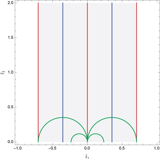
The shaded region is the fundamental region (47) and we plot the orbits on which the additional massless states appear in the first example. The three red lines correspond to condition 4 under which the gauge symmetry is enhanced to |$SO(16)\times SO(16)$|, and the one in the center implies the case of |$A=0$|. The two blue lines correspond to condition 4 under which the gauge symmetry is enhanced to |$SO(18)\times SO(14)$|. The green semicircles correspond to condition 4 and we plot four orbits with |$w_3=\pm1,\pm3$|.
We summarize the conditions under which the additional massless states appear. The cosmological constant is exponentially suppressed when the gauge group is enhanced to |$SO(14) \times SO(18)$|.
| Conditions | |$\tilde{\tau}_1=n_1/\sqrt{2}~$| (|$n_1\in\boldsymbol{Z}$|) | |$\tilde{\tau}_1=n_2/\sqrt{2}~$| (|$n_2\in\boldsymbol{Z}+1/2$|) |
|---|---|---|
| Gauge group | |$SO(16)\times SO(16)$| | |$SO(14) \times SO(18)$| |
| |$N_F-N_B$| | positive | zero |
| Conditions | |$\tilde{\tau}_1=n_1/\sqrt{2}~$| (|$n_1\in\boldsymbol{Z}$|) | |$\tilde{\tau}_1=n_2/\sqrt{2}~$| (|$n_2\in\boldsymbol{Z}+1/2$|) |
|---|---|---|
| Gauge group | |$SO(16)\times SO(16)$| | |$SO(14) \times SO(18)$| |
| |$N_F-N_B$| | positive | zero |
3.2. The interpolation between |$E_8 \times E_8$| and |$SO(16)\times SO(16)$|
Using the limiting behaviors of the boosted characters (56), we can see that this interpolating model (59) reproduces the supersymmetric |$E_8\times E_8$| model and the |$SO(16)\times SO(16)$| model as |$a\to 0$| and |$a\to \infty$| respectively, for any value of |$A$|.
3.2.1. The massless spectrum
Let us see the massless spectrum of this interpolating model for a generic set of values of |$a$| and |$A$|. By expanding the partition function (59) in |$q$|, we find
the 9D gravity multiplet: graviton |$G_{\mu \nu}$|, anti-symmetric tensor |$B_{\mu \nu}$|, and dilaton |$\phi$|;
the gauge bosons transforming in the adjoint representation of |$SO(16)\times SO(14)\times U(1)\times U(1)_{G,B}^{2}$|;
a spinor transforming in the |$(\boldsymbol{128},\boldsymbol{1})$| of |$SO(16)\times SO(14)$|.
These massless states come from |$\bar{V}_{8}O^{(0,0)}_{16}O_{16}$| or |$\bar{S}_{8}O^{(0,0)}_{16}S_{16}$|. For a generic set of values of |$a$| and |$A$|, |$N_F-N_B=-736$|, and the cosmological constant becomes negative. We find that there are some conditions between |$a$| and |$A$| under which the additional massless states appear:
(I) |$\tilde{\tau}_1=n_1/\sqrt{2}~~~~$| (|$n_1\in\boldsymbol{Z}$|)
Under this condition, we find that the following additional massless states appear:
two vectors transforming in the |$(\boldsymbol{1},\boldsymbol{14})$| of |$SO(16)\times SO(14)$|.
These massless vectors come from |$\bar{V}_{8} O^{(0,0)}_{16}O_{16}$| when |$(m,n)=(\pm1,\pm n_1)$| and |$w=0$|. This condition (I) thus enhances the gauge symmetry to |$SO(16)\times SO(16)\times U(1)_{G,B}^{2}$|. Furthermore, different additional massless states appear depending on whether |$n_1$| is even or odd:
(I-a) |$n_1\in 2\boldsymbol{Z}$|
two spinors transforming in the |$(\boldsymbol{1},\boldsymbol{64})$| of |$SO(16)\times SO(14)$|.
These states come from |$\bar{S}_{8} S^{(0,0)}_{16}O_{16}$| when |$(m,n)=(\pm1/2,\pm n_1/2)$| and |$w=0$|. In the representation of the |$SO(16)\times SO(16)$|, this is a spinor transforming in the |$(\boldsymbol{1},\boldsymbol{128})$|. Note that in the fundamental region (47), this condition corresponds to the |$\tilde{\tau}_1=0$| orbit, which means the case |$A=0$|. The massless spectrum under this condition is thus the same as that of the second example in Sect. 2.2.
(I-b) |$n_1\in 2\boldsymbol{Z}+1$|
two vectors transforming in the |$(\boldsymbol{1},\boldsymbol{64})$| of |$SO(16)\times SO(14)$|.
These states come from |$\bar{V}_{8} S^{(1/2,0)}_{16}O_{16}$| when |$(m,n)=(\pm1/2,\pm n_1/2)$| and |$w=0$|. In representation of the |$SO(16)\times SO(16)$|, this is a vector transforming in the |$(\boldsymbol{1},\boldsymbol{128})$|. Therefore, under this condition, the gauge symmetry is enhanced to |$SO(16)\times E_8$| beyond |$SO(16)\times SO(16)$|. Note that in the fundamental region (47), this condition corresponds to the |$\tilde{\tau}_1=\sqrt{2}/2$| (or |$\tilde{\tau}_1=-\sqrt{2}/2$|) orbit.
(II) |$\tilde{\tau}_1=n_2/\sqrt{2}~~~~$| (|$n_2\in\boldsymbol{Z}+1/2$|)
Under this condition, we find that the following additional massless states appear:
two spinors transforming in the |$(\boldsymbol{1},\boldsymbol{14})$| of |$SO(16)\times SO(14)$|.
These massless spinors come from |$\bar{S}_{8} O^{(1/2,0)}_{16}O_{16}$| when |$(m,n)=(\pm1,\pm n_2)$| and |$w=0$|. Note that in the fundamental region (47), this condition corresponds to the two orbits, which are |$\tilde{\tau}_1=\sqrt{2}/4$| and |$\tilde{\tau}_1=-\sqrt{2}/4$|.
(III) |$\frac{1}{\sqrt{2}}\tilde{\tau}_1-\left( \tilde{\tau}_{1}^2+\tilde{\tau}_{2}^2 \right)w_3=0 ~~~~$| (|$w_3\in2\boldsymbol{Z}+1$|)
The additional massless states are
two conjugate spinors transforming in the |$(\boldsymbol{16},\boldsymbol{1})$| of |$SO(16)\times SO(14)$|.
These massless conjugate spinors come from |$\bar{C}_{8} V^{(0,1/2)}_{16}V_{16}$| when |$(m,w)=\left( \pm1/2,\pm w_3\right) $| and |$n=0$|. Note that these conjugate spinors are the remnants of the |$\boldsymbol{8}_{C}\otimes (\boldsymbol{16},\boldsymbol{16})$| in the 10D |$SO(16)\times SO(16)$| model.
We plot these conditions in the fundamental region (47) of the |$\tilde{\tau}$| plane in Fig. 2. Table 2 summarizes the conditions under which the additional massless states appear in this model.
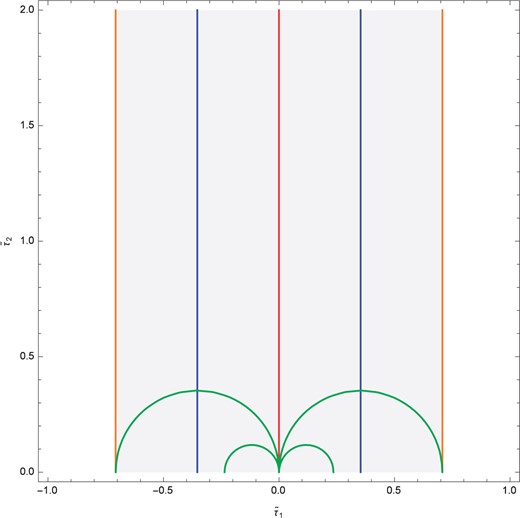
The shaded region is the fundamental region (47) and we plot the orbits on which additional massless states appear in the second example. The red line corresponds to condition (I) under which the gauge symmetry is enhanced to |$SO(16)\times SO(16)$|. The two orange lines correspond to condition (I) under which the gauge symmetry is enhanced to |$SO(16)\times E_8$|. The two blue lines correspond to condition (I). The green semicircles correspond to condition (I) and we plot four orbits with |$w_3=\pm1,\pm3$|.
We summarize the condition under which the additional massless states appear. In this model, there is no condition where the cosmological constant is exponentially suppressed.
| Conditions | |$\tilde{\tau}_1=n_1/\sqrt{2}~$| (|$n_1\in2\boldsymbol{Z}$|) | |$\tilde{\tau}_1=n_1/\sqrt{2}~$| (|$n_1\in2\boldsymbol{Z}+1$|) | |$\tilde{\tau}_1=n_2/\sqrt{2}~$| (|$n_2\in\boldsymbol{Z}+1/2$|) |
|---|---|---|---|
| Gauge group | |$SO(16)\times SO(16)$| | |$SO(16) \times E_8$| | |$SO(16)\times SO(14)\times U(1)$| |
| |$N_F-N_B$| | positive | negative | negative |
Finally, let us mention that in these models considered in this section, it is straightforward to calculate tree and one-loop scattering amplitudes of massless particles to obtain signals of broken supersymmetry [34–37].
4. Conclusions
We have constructed 9D interpolating models with two parameters by considering the compactification on a twisted circle with a constant Wilson line background (31), and have studied the massless spectra of these models. Furthermore, we have found some conditions between circle radius |$R$| and Wilson line |$A$| under which additional massless states are present. In the 9D model that interpolates between the 10D supersymmetric |$SO(32)$| model and the 10D |$SO(16)\times SO(16)$| model, we find the conditions under which the gauge symmetry is enhanced to |$SO(16)\times SO(16)$| or |$SO(18)\times SO(14)$|. In particular, under the second condition, the massless fermionic and bosonic degrees of freedom become equal, which means that the cosmological constant is exponentially suppressed. Recent references related to this point include Refs. [38–40]. According to Ref. [41], which is carried out in the type I dual picture [42], the brane configuration with the gauge group |$SO(18)\times SO(14)$| yields a 9D non-supersymmetric model with |$N_F-N_B=0$|, although it has tachyonic directions in moduli space. On the other hand, our interpolation between the 10D supersymmetric |$E_8\times E_8$| model and the 10D |$SO(16)\times SO(16)$| model did not produce a condition with |$N_F-N_B=0$|. We have, however, found the conditions under which the gauge symmetry is enhanced to |$SO(16)\times SO(16)$| or |$SO(16)\times E_8$|.
As part of our future work, we have to discuss the stability of the Wilson line as in Refs. [38–41]. Even if the cosmological constant is very small on a certain point (orbit) of moduli space, it is not clear that the Wilson line is stable on the point (orbit). Namely, we need to write down the cosmological constant in terms of the Wilson line and find the stable points of the Wilson line.
Acknowledgements
The work of H.I. was partially supported by Japan Society for the Promotion of Science (JSPS) KAKENHI Grant Number 19K03828.
Funding
Open Access funding: SCOAP|$^3$|.
Appendix A. Notation for the partition functions
Appendix B. The expansions of the characters
In string theories, we can see the spectrum of each mass level by expanding the partition function in |$q$|. In this appendix, in order to see the massless states, which are the coefficients of |$q^{0}$|, we shall expand the |$SO(8)$| and |$SO(16)$| characters, which appear in the partition function of some heterotic models5.
Appendix B.1. The case with no Wilson line
Note that the lowest-order terms of Eqs. (B.72), (B.73), and (B.74) correspond to the degrees of freedom of the identity, the vector, and the spinor (the conjugate spinor) respectively, and the second term of Eq. (B.72) to the adjoint representation of |$SO(2n)$|. The third term of |$\eta^{-8}O_{2n}$| comes from |$\eta^{-8}$|, i.e., the contributions from |$X^{m}$|.
Note that all states that come from |$\eta^{-8}V_{16}S_{16}$| or |$\eta^{-8}S_{16}S_{16}$| (|$\eta^{-8}S_{16}C_{16}$|) are massive, and tachyons can appear only from the combination |$\left( \eta\bar{\eta}\right)^{-8} \bar{O}_{8}O_{16}V_{16}$| because of the level-matching condition.
Appendix B.2. The case with the Wilson line
Note that no states that come from |$S^{(\alpha,\beta)}_{16}S_{16}$| (|$=S^{(\alpha,\beta)}_{16}C_{16}=C^{(\alpha,\beta)}_{16}S_{16}=C^{(\alpha,\beta)}_{16}C_{16}$|) or |$S^{(\alpha,\beta)}_{16}V_{16}$| (|$=C^{(\alpha,\beta)}_{16}V_{16}$|) will ever be massless.
Footnotes
2 It is not essential that a half translation |$\mathcal{T}$| is accompanied with the T-dualized coordinate |$\tilde{X}^9$|. If we adopted the ordinary coordinate |$X^9$|, the sum in Eq. (8) would be over |$n\in2(\boldsymbol{Z}+\alpha)$| and |$w\in\boldsymbol{Z}+\beta$|.
3 If the |$\boldsymbol{Z}_2$| twist |$\mathcal{T}Q$| acted trivially, then |$n$| and |$w$| would both be integers. Then, in addition to the shift (45), the momentum lattices would be invariant under |$\tilde{\tau} \to -1/\tilde{\tau}$| with the replacement |$n \leftrightarrow w$|. This transformation would correspond to a T-dual transformation, so the two limiting 10D models would be the same and the fundamental region would become |$-\sqrt{2}/2\leq\tilde{\tau}_1\leq\sqrt{2}/2$| and |$\left| \tilde{\tau} \right| \geq 1 $|.
5 There are five 10D heterotic models whose partition functions are expressed in terms of the characters |$SO(8)$| or |$SO(16)$|: the supersymmetric |$SO(32)$| model, the supersymmetric |$E_{8}\times E_{8}$| model, the non-supersymmetric |$SO(32)$| model, the |$SO(16)\times E_8$| model, the |$SO(16)\times SO(16)$| model.
