


Abstract
To analyze trajectories for systems of many degrees of freedom, we propose a new method called wavelet local principal component analysis (WlPCA) combining the wavelet transformation and local PCA in time. Our method enables us to reduce the dimensionality of time series both in degrees of freedom and frequency so that characteristic features of oscillatory behavior can be captured. To test the new method, we apply WlPCA to a non-autonomous model of multiple degrees of freedom, the Froeschlé maps of |$N=2$| and |$N=4$|, which correspond to autonomous systems of three and five degrees of freedom, respectively. The eigenvalues and eigenvectors obtained by WlPCA reveal those times when frequency variation exhibits switching between relatively stationary features. Moreover, further analyses indicate which degrees of freedom and frequencies are involved in the switching. We confirm that the switching corresponds to the onset of transport in phase space. These findings imply that, even for systems of larger degrees of freedom, barriers can exist in phase space that block transport for a finite time, thereby dividing the phase space into multiple quasi-stationary regions. Thus, our method is promising for understanding dynamics in systems of many degrees of freedom, such as vibrational-energy redistribution in molecules.
1. Introduction
Analysis of phase space structure plays an important role in various research fields such as chemical reactions [1], celestial mechanics [2,3], plasma physics [4] and fluid dynamics [5,6]. To understand dynamical behavior in these fields, we need to investigate how trajectories wander around from region to region in phase space. When the system is strongly chaotic, transport processes in phase space are so frequent that only time-averaged quantities would be of interest. Then, statistical approaches could be applied to extract essential features of the dynamics. On the other hand, when chaos is not so efficient for mixing in phase space, more elaborate methods would be necessary to reveal the dynamical aspects of the system.
For systems of two degrees of freedom, the Poincaré section plays a key role. Since the Poincaré section is 2D, we can visualize the phase space, and detailed analysis of the phase space structure is possible for the mixed phase space, i.e., when tori and chaos coexist. Then, the Kolmogorov–Arnold–Moser (KAM) torus [7,8] divides the phase space into separate regions and works as a barrier for the transport processes [9]. Moreover, so-called remnant tori are known to play the role of partial barriers for mixing [10], and accumulation of higher-order tori is believed to give rise to stagnant behavior near the resonant tori [11,12].
For systems of more than two degrees of freedom, the KAM tori no longer play the role of barriers in phase space because of the following reason. Let |$N$| denote the degree of freedom of the system. Then, the dimension of the phase space is |$2N$| and that of the equi-energy surface is |$2N-1$|. The Poincaré section on the equi-energy surface is |$2N-2$|D. Since the dimension of the KAM tori is |$N-1$| on the |$2N-2$|D Poincaré section, they do not divide the phase space of the section into two separate regions when |$N>2$|.
This leads to dynamical properties called Arnold diffusion [13–23], which does not exist for systems of two degrees of freedom. Arnold diffusion is movement along resonance surfaces and is supposed to be important for near-integrable systems. However, for a mixed phase space in general, transport processes across resonance surfaces are shown to be more frequent than Arnold diffusion [24–26]. Moreover, recent studies of transport processes reveal that trajectories are trapped around resonance junctions, where multiple resonances meet on the action space [27]. They study systems of three degrees of freedom and focus their attention on the Arnold web, i.e., the web composed of resonance surfaces on the action space (or, precisely speaking, on the frequency space). The reason for this is that, for |$N=3$|, the dimension of the action space is three so that the Arnold web can be visualized there. Note that the Poincaré section for |$N=3$| is 4D and cannot be shown as it is.
Stagnant behavior is also of interest for systems of more than two degrees of freedom [28]. For |$N=2$|, fractal-like accumulation of partial barriers is supposed to give rise to fractional behavior of the dynamics [11,12]. Note that this mechanism is specific to systems of two degrees of freedom. However, some studies indicate that fractional behavior can also be seen in a mixed phase space even for |$N>2$| [29–31]. These results raise a question of whether the mechanism of the stagnant behavior for |$N=2$| is generic or not. In order to understand the mechanism of the stagnant behavior for |$N>2$|, we need to analyze the phase space rather than the action space. Recent studies for |$N=3$| employ 3D sections of the 4D Poincaré section and shed new light on the stagnant behavior of the dynamics [32,33].
In the study of dynamics in general, one of the key concepts is normally hyperbolic invariant manifolds (NHIMs) [34–38]. Their stable/unstable manifolds and the intersection between stable and unstable manifolds give a basic mechanism of transport in phase space [39–42]. They play an important role in recent studies of chemical reactions [43–48] and celestial mechanics [49–52]. The analysis of NHIMs for |$N=3$| leads us to find a new phenomenon called switching of reaction coordinates [53–56]. This phenomenon is generic for systems of more than two degrees of freedom and would give rise to new mechanisms in various areas including chemical reactions.
Thus, a new wave of research into dynamical behavior of Hamiltonian dynamics is appearing these days. However, analysis of the dynamics of systems of even larger degrees of freedom still remains challenging although various approaches have been tried [57–65].
The purpose of this paper is to propose a new approach toward the phase space structure utilizing the methodology of time series analysis. Combining time–frequency analysis and dimensionality reduction, we develop a new method to analyze transport processes in phase space. Here, we employ the wavelet transformation [66–68] for the time–frequency analysis and principal component analysis (PCA) for dimensionality reduction so that we can reveal how transport in phase space and change of frequency correspond with each other. The wavelet transformation has been applied to analyze the dynamical behavior of chaos [30,69,70]. However, it has not been combined with the methods of dimensional reduction so far in the study of chaos. Employing the dimensional reduction both in degrees of freedom and frequency, our method would extract which degrees of freedom participate in a exchange of vibrational energy and which frequency ranges are used in that exchange. Moreover, applying the method locally in time would make it possible to reveal nonstationary features in the exchange. Thus, the method would be suitable to see if stagnant behavior exists for systems of larger degrees of freedom and to investigate how transition among such stagnant motion takes place, if any.
The paper is organized as follows. In Sect. 2, we explain our method of combining the wavelet transformation and principal component analysis (PCA). After introducing the wavelet transformation in Sect. 2.1 and PCA in Sect. 2.2, we present the wavelet local principal component analysis (WlPCA) in Sect. 2.3. In Sect. 3, we explain a model system called the Froeschlé map [71] in an extended form that consists of |$N$| standard maps interacting with each other. In Sect. 4, we apply WlPCA to the Froeschlé map of |$N=2$| to see how the eigenvalues and eigenvectors obtained by WlPCA reveal dynamical changes of oscillatory motions. In particular, we notice that the oscillatory motions exhibit both relatively stationary features and switching between them. Introducing a procedure to detect when the switching takes place, we confirm that the switching actually corresponds to the onset of transport processes between regions in phase space. In Sect. 5, we verify that our method also works to reveal the switching for the Froeschlé map of |$N=4$|. This suggests that, even for systems of larger degrees of freedom, barriers for transport can exist, giving rise to nonstationary features in the oscillatory behavior. In Sect. 6, we summarize our results and discuss future prospects for extending our method.
2. Method
Our method is a combination of the wavelet transformation and PCA, where PCA is applied locally in time. Therefore, we call it the wavelet local PCA (WlPCA). In this section, after introducing the wavelet transformation and PCA, we present our method, the WlPCA.
2.1. Wavelet transformation
The wavelet transformation is an extension of the Fourier transformation to nonstationary time series. Intuitively speaking, the wavelet transformation is regarded as a windowed Fourier transformation, where the width of the window is adjusted according to the frequency of oscillation.
In Eq. (3), the width of the window in time is |$2\sigma/\omega$|, and the period of oscillation with its frequency |$\omega$| is |$2\pi/\omega$|. Therefore, the number of waves in the window for oscillations of frequency |$\omega$| is estimated to be |$\sigma/\pi$|. Note that its value does not depend on |$\omega$|. This enables us to apply the Morlet wavelet transformation to time series with a wide range of frequencies. In our analysis here, we set |$\sigma=36$|.
In actual application, the length of a times series is finite with finite sampling steps. Then, we need to pay attention to artifacts caused by these limitations. In particular, discontinuity at the boundaries of the time series could cause pronounced values of the wavelet transformation for smaller values of frequencies. In our analysis, we do not use the values of the wavelet transformation for lower frequency ranges that cause this artifact.
2.2. Principal component analysis (PCA)
Principal component analysis (PCA) is used for dimensionality reduction. For a given distribution of data points in a certain space of large dimension, the analysis extracts a representation of the data in a space of reduced dimensionality.
Let us choose the space |${\bf V}^{(D)}$| spanned by the eigenvectors |${\bf v}^{(1)},{\bf v}^{(2)},\ldots,$| and |${\bf v}^{(D)}$|. When we project the vectors of the set |$S$| onto the space |${\bf V}^{(D)}$|, we obtain their representation with a reduced dimension |$D$| in the space |${\bf V}^{(D)}$|. This is the basic idea of PCA.
2.3. Wavelet local PCA (WlPCA)
In the following, we think of a time series |${\bf x}\left(s\right)$| in an |$N$|D space |${\bf R}^N$| and apply the wavelet transformation to each of its components |$x_i\left(s\right)$| to obtain |${\tilde x}_i\left(\omega,t\right)$|, where |$i=1,2,\ldots,N$|. In the actual calculation, the length of the time series is finite with a finite time step. Therefore, the wavelet transformation |${\tilde x}_i\left(\omega,t\right)$| is estimated only at discretized values of frequency and time |$\left(\omega_l,t_m\right)$|.
In the following, we analyze the wavelet spectra |$\left|{\tilde x}_i\left(\omega_l,t_m\right)\right|^2$|, and, in PCA, we treat the wavelet spectra as a vector |${\bf X}(t_m)$|, where its components are indexed using the composed suffix |$j=(i,l)$| as |$X_{j=(i,l)}(t_m)=\left|{\tilde x}_i\left(\omega_l,t_m\right)\right|^2$|. Let |$L$| denote the number of frequencies where the wavelet transformation is estimated. Then, the dimension of the wavelet spectra |${\bf X}(t_m)$| is |$J=LN$|.
After diagonalizing the matrix |$\Sigma(t')$|, we obtain its eigenvalues |$\lambda^{(n)}(t')$| and their corresponding eigenvectors |${\bf v}^{(n)}(t')$|. We show a schematic picture of the above idea in Fig. 1. In our analysis, we fix the width |$T$| and change the time |$t'$|. Therefore, in Eq. (8), we do not show explicitly the dependence on the width |$T$|.
![A schematic picture of wavelet local principal component analysis (WlPCA). We perform PCA locally in time over the interval $I_{t'}=[t'-T/2,t'+T/2]$ to see how the eigenvalues $\lambda^{(n)}(t')$ and their corresponding eigenvectors ${\bf v}^{(n)}(t')$ vary as we change the center $t'$ of the interval $I_{t'}$.](https://oup.silverchair-cdn.com/oup/backfile/Content_public/Journal/ptep/2019/12/10.1093_ptep_ptz129/4/m_ptz129f1.jpeg?Expires=1750479393&Signature=qEC2-JKv5U5TEtugEM8-hxV5Y7gpP1f~9TNiITT4hxdDt5477LG-u7zfENdDcRSj00QKXb9zalR9110ByYiz5fOPI-7egrzKV2xrs07wjP3SCuxkswA0UD1MZt4CX2eU2dw98T8jnqjuwYu-HEjXU4~YXpq9OKslKVZEkqW1KLMdrbZe-VFpdQqAv-lQaxTx2c2AmB04TdenGsthuUwLh~QePBahRscgkieCWw9If2hIZ5jgZMKhHjI1XPTO80iKzbh~-xp7Eg405L~At2AIwV-IMJ3~EB8ifXGI2xvlsdpCf6xkZLr7RdyjhMviG~sySO~EJMMI47WO~w~oTmvefQ__&Key-Pair-Id=APKAIE5G5CRDK6RD3PGA)
A schematic picture of wavelet local principal component analysis (WlPCA). We perform PCA locally in time over the interval |$I_{t'}=[t'-T/2,t'+T/2]$| to see how the eigenvalues |$\lambda^{(n)}(t')$| and their corresponding eigenvectors |${\bf v}^{(n)}(t')$| vary as we change the center |$t'$| of the interval |$I_{t'}$|.
Our WlPCA method performs dimensional reduction for both degrees of freedom and frequencies. The eigenvalues and eigenvectors thus obtained provide us with information concerning correlation among vibrational motions involving specific degrees of freedom and frequencies.
3. Model Hamiltonian
In its original form, the Froeschlé map consists of two standard maps interacting with each other, and is a model of 2.5 degrees of freedom, i.e., a system of two degrees of freedom under periodic external force. Therefore, the strobe map of this model corresponds to the Poincaré map for autonomous systems of three degrees of freedom. It is suitable for studying dynamical behavior such as Arnold diffusion, which is specific to systems of more than two degrees of freedom [24–26,71–74]. In this paper, we use the Froeschlé map [71] with |$N=2$| and |$N=4$| to investigate whether our method can reveal information concerning the phase space structure for systems of larger degrees of freedom.
4. Results for a system of 2.5 degrees of freedom
In this chapter, we set |$N=2$|, i.e., a system of |$2.5$| degrees of freedom, which corresponds to an autonomous system of |$3$| degrees of freedom.
4.1. Time evolution of eigenvalues and eigenvectors
In this section, we use WlPCA to analyze time series of |$p_i(t)$| for |$i=1,2$| of the Froeschlé map with |$K=0.8$| and |$b=0.002$|. After their wavelet transformations |${\tilde p}_i\left(\omega_l,t_m\right)$| are obtained, we apply local PCA to the wavelet spectra |${\bf P}(t_m)$|, where its |$j=(i,l)$|th component is defined by |$P_{j=(i,l)}(t_m)=\left|{\tilde p}_i\left(\omega_l,t_m\right)\right|^2$|. In the following, we choose the width of the interval |$I_{t'}$| for a time average as |$T=2000$| steps. Then, the eigenvalues |$\lambda^{(n)}(t')$| and their corresponding eigenvectors |${\bf v}^{(n)}(t')$| are obtained by WlPCA.
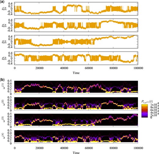
First, we see how the largest eigenvalue |$\lambda^{(1)}(t')$| changes as we vary the center of the interval |$I_{t'}$|. In Fig. 2, we display time series of |$p_i(t)$| for |$i=1,2$| of the Froeschlé map with |$K=0.8$| and |$b=0.002$|, their wavelet spectra |$\left|\tilde p_i\left(\omega,t\right)\right|^2$|, time series of the largest eigenvalue |$\lambda^{(1)}(t')$|, and that of the contribution ratio |$\mu^{(1)}(t')$| of the largest eigenvalue, where the contribution ratio of the |$n$|th eigenvalue is defined by |$\mu^{(n)}(t')=\lambda^{(n)}(t')/\left(\sum_{j=1}^{J}\lambda^{(j)}(t')\right)$|.
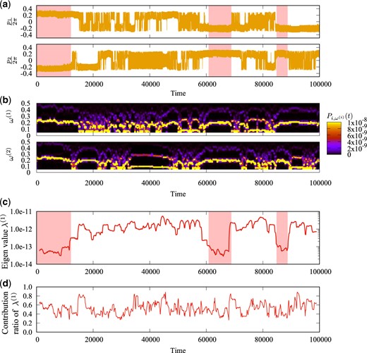
(a) Time series of |$p_i(t)$| for |$i=1,2$| of the Froeschlé map with |$N=2$|, |$K=0.8$|, and |$b=0.002$|. (b) Wavelet spectra |$\left|\tilde p_i\left(\omega,t\right)\right|^2$|, where |$\tilde p_i\left(\omega,t\right)$| denotes the wavelet transformation of |$p_i(t)$| for |$i=1,2$|. (c) Time series of the largest eigenvalue |$\lambda^{(1)}(t')$|, where |$t'$| indicates the center of the interval |$I_{t'}$| for the time average. The width of the interval is set to be |$T=2000$| steps. (d) Time series of the contribution ratio of the largest eigenvalue, |$\mu^{(1)}(t')=\lambda^{(1)}(t')/\left(\sum_{j=1}^{J}\lambda^{(j)}(t')\right)$|.
In Fig. 2(a), we shade those time regions when relatively stable oscillatory motion continues for both |$i=1,2$|. Then, variation of their wavelet spectra |$\left|\tilde p_i\left(\omega,t\right)\right|^2$| is relatively modest, and the value of the first eigenvalue |$\lambda^{(1)}(t')$| is smaller than other time regions. This implies that the first eigenvalue is a good indicator of how oscillatory motion varies in time. Moreover, Fig. 2(d) shows that |$\mu^{(1)}(t')\gtrsim 0.4$| almost always holds, which means that the reduction of dimensionality is efficient even in the 1D space spanned only by the first eigenvector.
In Fig. 3, we compare the time series of the |$j$|th component |$v_{j=(i,l)}^{(1)}(t')$| of the first eigenvector |${\bf v}^{(1)}(t')$| with that of the average wavelet spectra |$\left<P_{j=(i,l)}\right>_{t',T}$|. In Fig. 4, as an example, we give our attention to the time |$t'=84\,700$| to see how the first eigenvector reflects the variation of the average wavelet spectra in time from |$t'=83\,700$| to |$t'=85\,700$|. In the right figure of Fig. 4(a), the first eigenvector at |$t'=84\,700$| reveals pronounced changes in its peaks for the |$j=(i=1,l)$|th components, i.e., the components for |$p_1$|. These changes reflect those in the strength of the wavelet spectra for |$i=1$| from |$t'=83\,700$| to |$t'=85\,700$|, as is shown in the right column of Fig. 4(b). For |$i=2$| in Fig. 4(b), we can also see that the widths of the spectra of |$i=2$| shrink from |$t'=83\,700$| to |$t'=85\,700$|. This change is revealed in the first eigenvector for the |$j=(i=2,l)$|th components. Thus, the first eigenvector characterizes how the average wavelet spectra vary in time.
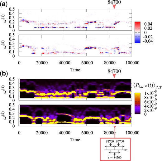
(a) The |$j$|th component |$v_{j=(i,l)}^{(1)}(t')$| of the first eigenvector |${\bf v}^{(1)}(t')$|. (b) The average wavelet spectra |$\left<P_{j=(i,l)}\right>_{t'}$|, where the time average is taken over the interval |$I_{t'}$| with |$T=2000$| steps. For both (a) and (b), the upper figures are for |$i=1$| and the lower ones for |$i=2$|, respectively. The ordinate and abscissa of these figures are the frequency |${\omega_l}^{(i)}$| and the time |$t'$|, respectively, where |${\omega_l}^{(i)}$| denotes the frequency of the |$i$|th momentum |$p_i$|. The arrows in these figures indicate the time |$t'$| when the eigenvector is displayed in Fig. 4.
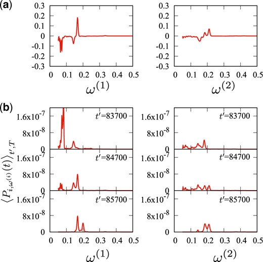
(a) The |$j$|th component |$v_{j=(i,l)}^{(1)}(t')$| of the first eigenvector |${\bf v}^{(1)}(t')$| at |$t'=84\,700$| indicated by the arrow in Fig. 3(a). Their ordinate and abscissa are the |$j$|th component |$v_{j=(i,l)}^{(1)}(t')$| of the first eigenvector |${\bf v}^{(1)}(t')$| and the frequency |${\omega_l}^{(i)}$|. (b) The average wavelet spectra |$\left<P_{j=(i,l)}\right>_{t',T}$| at |$t'$| indicated in Fig. 3(b). Their ordinate and abscissa are the average wavelet spectra |$\left<P_{j=(i,l)}\right>_{t',T}$| and the frequency |${\omega_l}^{(i)}$|. For both (a) and (b), the left figures are for |$i=1$| and the right ones for |$i=2$|. Comparing (a) and (b), we can see that the components of the first eigenvector at |$t'=84\,700$| correspond to changes of the average wavelet spectra taking place from |$t'=83\,700$| to |$t'=85\,700$|.
4.2. Switching of oscillatory motion
The results of the previous section indicate that the first eigenvector of WlPCA characterizes how the average wavelet spectra change and which degrees of freedom and frequencies are involved in these changes. Generally speaking, in chaotic dynamical systems, various changes can take place on multiple timescales. Here, our purpose is to detect those changes occurring on specific timescales.
In Fig. 5, we show the time series of the first and second eigenvalues |$\lambda^{(1)}(t')$| and |$\lambda^{(2)}(t')$|, the absolute value of the inner product |$\left|{\bf v}^{(1)}({t_1}')\cdot{\bf v}^{(1)}({t_2}')\right|$| between the first eigenvectors at different times, |${t_1}'$| and |${t_2}'$|, and the time series of the momenta |$p_i(t)$| for |$i=1,2$|. In Fig. 5(a), there exist multiple avoided crossings between the first and second eigenvalues. This phenomenon is reminiscent of the crossing of eigenvalues in adiabatic transition, chemical bonding, and quantum chaos. These avoided crossings suggest that the first eigenvector |${\bf v}^{(1)}(t')$| and the second one |${\bf v}^{(2)}(t')$| exchange with each other around there. Such exchanges can be confirmed by calculating the inner product between the first eigenvectors at different times, |${\bf v}^{(1)}({t_1}')$| and |${\bf v}^{(1)}({t_2}')$|. In Fig. 5(b), the values of the inner product reveal clustering of similar first eigenvectors implying that oscillatory behavior in these time ranges has similar features in common. In other words, the characteristics of oscillatory motions captured by the first eigenvector can be classified according to the values of the inner product. Moreover, these classes exhibit hierarchical structures, possibly reflecting hierarchical structures of the phase space.
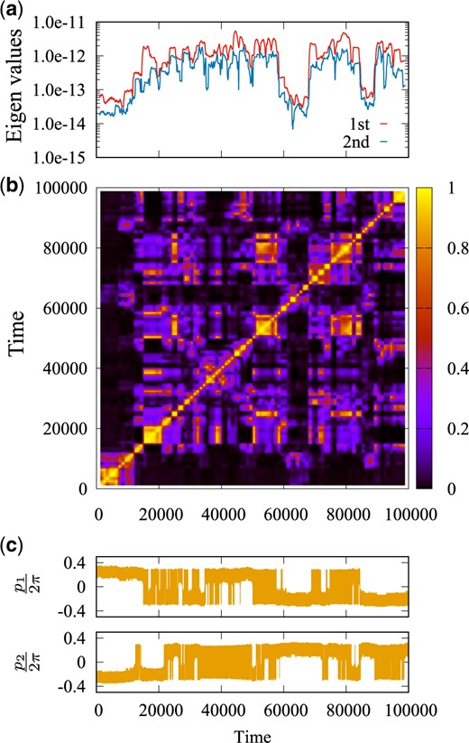
(a) The time series of the first and second eigenvalues, |$\lambda^{(1)}(t')$| and |$\lambda^{(2)}(t')$|. The plot for |$\lambda^{(1)}(t')$| is the same as Fig. 2(c). (b) The absolute value of the inner product |$\left|{\bf v}^{(1)}({t_1}')\cdot{\bf v}^{(1)}({t_2}')\right|$| between the first eigenvectors at different times |${t_1}'$| and |${t_2}'$|. (c) Time series of |$p_i(t)$| for |$i=1,2$| of the Froeschlé map. It is the same as Fig. 2(a).
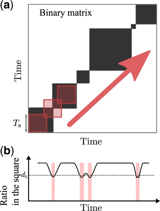
Schematic explanation of how to detect switching taking place with a specific timescale |$T_{\rm s}$|. (a) Clustering structure in the binary representation |$u\left({t_1}',{t_2}'\right)$| is scanned along the diagonal line |${t_1}'={t_2}'$| using a square with the length of its sides |$T_{\rm s}$|, which is the timescale of interest. (b) Time series of the ratio |$d(t')$| of those pairs |$({t_1}',{t_2}')$| satisfying |$u\left({t_1}',{t_2}'\right)=1$| within the square with its center at |$t'$|. Switching in the clustering structure can be detected using the condition of |$d(t')<d_{\rm T}$|, where |$d_{\rm T}$| is the threshold to locate the downward tips in the variation of |$d(t')$|.
In Fig. 7, we display the results to detect changes for the inner product shown in Fig. 5(b). We depict, in Fig. 7(a), the binary representation obtained from Fig. 5(b) using the value of the threshold |$u_{\rm T}=0.1$|. We can see the hierarchy of clustering structures implying that oscillatory motions share common features over various timescales. In Fig. 7(b), we depict the time series of the ratio |$d(t')$| for the binary representation shown in Fig. 7(a) choosing the length of the sides of the square |$T_{\rm s}=1400$| steps. Then, we notice that |$d(t')$| exhibits a wedge-shaped decrease at several times signifying that there exists switching in the oscillatory behavior; i.e., a sharp transition takes place there between relatively stationary features. In Fig. 7(b), nine switchings are detected using the condition |$d(t')<d_{\rm T}$| where we set |$d_{\rm T}=0.75$|. These switchings are indicated by the shaded lines there.
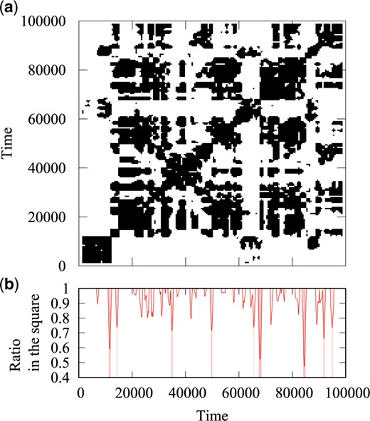
(a) Binary representation of the figure of the inner products shown in Fig. 5(b). The value of the threshold is |$u_{\rm T}=0.1$|. (b) Time series of the ratio |$d(t')$| for the binary representation. The length of the sides of the square is |$T_{\rm s}=1400$| steps. We can see a wedge-shaped decrease at several times signifying switching in the oscillatory behavior. Nine switchings are detected using the condition |$d(t')<d_{\rm T}$| where we set |$d_{\rm T}=0.75$|. These switchings are indicated by the shaded lines.
These detected switchings are shown in Fig. 8, where we display the time series of the first and second eigenvalues |$\lambda^{(1)}(t')$| and |$\lambda^{(2)}(t')$|. We see that these switchings correspond well to avoided crossings although all of the crossings are not detected as switching because of the condition of the timescales. In Fig. 7(b), these exist some downward tips whose values of |$d(t')$| do not satisfy the condition |$d(t')<d_{\rm T}$| with |$d_{\rm T}=0.75$|, implying that they are excluded by the condition of the timescales.
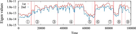
Time series of the first and second eigenvalues |$\lambda^{(1)}(t')$| and |$\lambda^{(2)}(t')$| with the nine switchings detected.
We analyze in more detail those switchings with lower values of |$d(t')$| to see what kind of changes take place. For example, we choose the switching at |$t'=11\,540$| in the following. In Fig. 9(a), we show time series of the first and second eigenvalues |$\lambda^{(1)}(t')$| and |$\lambda^{(2)}(t')$| magnified around |$t'=11\,540$|. There, we can see that, at |$t'=11\,540$|, a close avoided crossing takes place, implying that exchange between the first and second eigenvectors occurs there. In Fig. 9(b), we display time series of the wavelet spectra |$\left|\tilde p_i\left(\omega,t\right)\right|^2$| for |$i=1,2$| around |$t'=11\,540$|. We can see that the spectra for |$i=2$| change their characteristic features around |$t'=12\,000$| from a relatively modest variation to a more violent one. On the other hand, the spectra for |$i=1$| remain modest throughout the whole range of time shown there. Note that, in the WlPCA here, the time average is taken over the interval with its width |$T=2000$| steps. Therefore, the switching of the eigenvalues at |$t'=11\,540$| reflects the changes taking place over the interval |$I_{t'=11\,540}$|, which covers the range of time when the spectra of |$i=2$| start to exhibit violent variation.
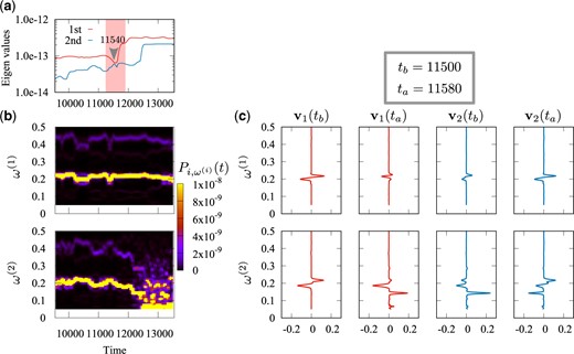
(a) Time series of the first and second eigenvalues |$\lambda^{(1)}(t')$| and |$\lambda^{(2)}(t')$| magnified around |$t'=11\,540$|. At |$t'=11\,540$|, a close avoided crossing takes place, implying that exchange between the first and second eigenvectors occurs there. (b) Time series of the wavelet spectra |$\left|\tilde p_i\left(\omega,t\right)\right|^2$| for |$i=1,2$| around |$t'=11\,540$|. (c) Comparison between the first and second eigenvectors before and after the switching, i.e., |$t_{\rm b}=11\,500$| and |$t_{\rm a}=11\,580$|, respectively.
In Fig. 9(c), we display the first and second eigenvectors before and after the switching, i.e., |$t_{\rm b}=11\,500$| and |$t_{\rm a}=11\,580$|, respectively. Comparing the first eigenvector before the switching |${\bf v}^{(1)}(t_{\rm b})$| and the second one after the switching |${\bf v}^{(2)}(t_{\rm a})$|, we notice that they appear to be quite similar. The second eigenvector before the switching |${\bf v}^{(2)}(t_{\rm b})$| and the first one after the switching |${\bf v}^{(1)}(t_{\rm a})$| also exhibit a close resemblance to each other. Thus, we confirm that the exchange of the first and second eigenvectors takes place at |$t'=11\,540$|. Moreover, the peak for |$\omega^{(i=2)}$| slightly above |$0.2$| of the first eigenvector before the switching |${\bf v}^{(1)}(t_{\rm b})$| decreases in the first eigenvector after the switching |${\bf v}^{(1)}(t_{\rm a})$|, and a new peak around |$\omega^{(i=2)}\sim 0.15$| appears in the first eigenvector after the switching |${\bf v}^{(1)}(t_{\rm a})$|. These phenomena closely reflect the changes taking place in the wavelet spectra |$\left|\tilde p_{i=2}\left(\omega,t\right)\right|^2$| around |$t'=12\,000$|. Thus, the first eigenvector obtained by WlPCA exhibits characteristics of changes taking place in the wavelet transformation.
We can confirm how the switching detected at |$t'=11\,540$| appears as the onset of transport in the phase space. In Fig. 10, the trajectory is shown in the phase space around |$t'=11\,540$|. The upper figures show the points |$(q_i(t),p_i(t))$| of the trajectory for |$i=1$|, and the lower ones those for |$i=2$|. The figures in the left column show the plot before the switching, i.e., the points from |$t=9540$| to |$t=11\,540$|; those in the right column show that after the switching, i.e., the points from |$t=11\,540$| to |$t=13\,540$|. We see that the areas in the phase space visited by the trajectory differ between before and after the switching for |$i=2$|. Thus, the switching reveals the onset of transport processes taking place between quasi-stationary regions in the phase space.

The switching taking place around |$t'=11\,540$| in phase space. The upper figures show the points of the trajectory for |$i=1$| and the lower ones those for |$i=2$|. The figures in the left column show the plot before the switching, i.e., the points from |$t=9540$| to |$t=11\,540$|; those in the right column show that after the switching, i.e., the points from |$t=11\,540$| to |$t=13\,540$|.
In Fig. 11, the switching at |$t'=11\,540$| detected in Fig. 7 is shown by the arrow on the frequency plane |$(\omega^{(1)},\omega^{(2)})$|. There, we plot time series of the local frequencies defined by |$\omega^{(i)}(t')=\mathop{\rm arg~max}\limits_{\omega_l}v_{j=(i,l)}^{(1)}(t')$| for |$i=1,2$|. Dots with different colors indicate that they belong to those regions of time separated by the switching at |$t'=11\,540$|. We can see that the classification of local frequencies corresponds to different features of the oscillatory behavior. Thus, our method enables us to capture switching of the oscillatory motions both in phase space and frequency space.
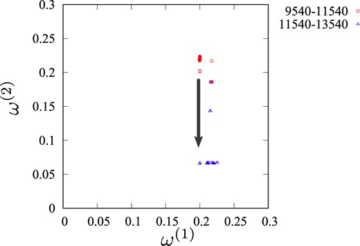
Time series of the local frequencies defined by |$\omega^{(i)}(t')=\mathop{\rm arg~max}\limits_{\omega_l}\left|v_{j=(i,l)}^{(1)}(t')\right|$| for |$i=1,2$| plotted on the frequency plane |$(\omega^{(1)},\omega^{(2)})$|. Dots with different colors indicate that they belong to those regions of time separated by the switching at |$t'=11\,540$| detected in Fig. 7. The switching at |$t'=11\,540$| is shown by the arrow.
5. Results for a system of 4.5 degrees of freedom
In this chapter, we set |$N=4$|, i.e., a system of |$4.5$| degrees of freedom, which corresponds to an autonomous system of |$5$| degrees of freedom.
5.1. Time evolution of eigenvalues and eigenvectors
In Fig. 12, we show time series of |$p_i(t)$| for |$i=1,\ldots,N$| of the Froeschlé map with |$N=4$|, |$K=0.5$|, and |$b=0.02$|, and the wavelet spectra |$\left|\tilde p_i\left(\omega,t\right)\right|^2$|, where |$\tilde p_i\left(\omega,t\right)$| denotes the wavelet transformation of |$p_i(t)$| for |$i=1,\ldots,N$|. We can see that the wavelet spectra exhibit modest variations in some regions in time while in other regions they reveal violent changes. Thus, the trajectory shows nonstationary features in its oscillatory behavior.
(a) Time series of |$p_i(t)$| for |$i=1,\ldots,N$| of the Froeschlé map with |$N=4$|, |$K=0.5$|, and |$b=0.02$|. (b) Wavelet spectra |$\left|\tilde p_i\left(\omega,t\right)\right|^2$|, where |$\tilde p_i\left(\omega,t\right)$| denotes the wavelet transformation of |$p_i(t)$| for |$i=1,\ldots,N$|.
In Fig. 13(a), we display time series of the largest eigenvalue |$\lambda^{(1)}(t')$|, where |$t'$| indicates the center of the interval |$I_{t'}$| for the time average. The width of the interval is set to be |$T=2000$| steps. In Fig. 13(b), we show time series of the contribution ratio of the largest eigenvalue, |$\mu^{(1)}(t')=\lambda^{(1)}(t')/\left(\sum_{j=1}^{J}\lambda^{(j)}(t')\right)$|. As is the result for the system with |$N=2$|, the contribution ratio of the first eigenvalue attains the value |$\mu(t')^{(n=1)}\sim 0.4$| for almost all times. In Fig. 13(c), we show the |$j$|th component |$v_{j=(i,l)}^{(1)}(t')$| of the first eigenvector |${\bf v}^{(1)}(t')$| for |$i=1,\ldots,N$|. Variation of the components of the first eigenvector indicates which degrees of freedom exhibit violent behavior in their oscillatory motions. We also notice that there exist sharp changes when some degrees of freedom cease to exhibit violent behavior and other ones start to show it. Thus, we expect that switching also takes place for |$N=4$|, and that such switching would reveal richer features than that for |$N=2$|.
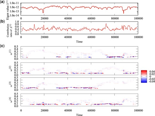
(a) Time series of the largest eigenvalue |$\lambda^{(1)}(t')$|, where |$t'$| indicates the center of the interval |$I_{t'}$| for the time average. The width of the interval is set to be |$T=2000$| steps. (b) Time series of the contribution ratio of the largest eigenvalue, |$\mu^{(1)}(t')=\lambda^{(1)}(t')/\left(\sum_{j=1}^{J}\lambda^{(j)}(t')\right)$|. (c) The |$j$|th component |$v_{j=(i,l)}^{(1)}(t')$| of the first eigenvector |${\bf v}^{(1)}(t')$| for |$i=1,\ldots,N$|.
5.2. Switching of oscillatory motion
In Fig. 14(a), we show time series of the first and second eigenvalues |$\lambda^{(1)}(t')$| and |$\lambda^{(2)}(t')$|. There, many avoided crossings take place, implying that exchange between the first and second eigenvectors occurs there, as we can expect from Fig. 13(c). In Fig. 14(b), we show the absolute value of the inner product |$\left|{\bf v}^{(1)}({t_1}')\cdot{\bf v}^{(1)}({t_2}')\right|$| between the first eigenvectors at different times |${t_1}'$| and |${t_2}'$|. In Fig. 14(d), we show a binary representation of the figure of the inner products shown in Fig. 14(b), where the value of the threshold is |$u_{\rm T}=0.1$|. In Fig. 14(c), we show time series of the ratio |$d(t')$| for the binary representation shown in Fig. 14(d) with the length of the sides of the square |$T_{\rm s}=1000$| steps. As in Fig. 7(b), |$d(t')$| here exhibits a wedge-shaped decrease, indicating the existence of switching in the oscillatory behavior. In Fig. 14(c), eight switchings are detected using the condition |$d(t')<d_{\rm T}$| where we set |$d_{\rm T}=0.75$|, as shown by the shaded lines.
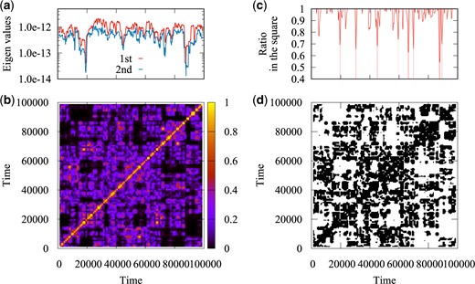
(a) Time series of the first and second eigenvalues |$\lambda^{(1)}(t')$| and |$\lambda^{(2)}(t')$|. We can see that many avoided crossings take place, implying that exchange between the first and second eigenvectors occurs there. (b) The absolute value of the inner product |$\left|{\bf v}^{(1)}({t_1}')\cdot{\bf v}^{(1)}({t_2}')\right|$| between the first eigenvectors at different times |${t_1}'$| and |${t_2}'$|. (c) Time series of the ratio |$d(t')$| for the binary representation shown in Fig. 14(d) with the length of the sides of the square |$T_{\rm s}=1000$| steps. Eight switchings are detected using the condition |$d(t')<d_{\rm T}$| where we set |$d_{\rm T}=0.75$|. (d) Binary representation of the figure of the inner products shown in Fig. 14(b) with the value of the threshold |$u_{\rm T}=0.1$|.
In Fig. 15, we show the switching taking place at |$t'=30\,540$| in more detail. In Fig. 15(a), we compare the first eigenvectors before and after the switching, i.e., |$t_{\rm b}=28\,540$| and |$t_{\rm a}=32\,540$|, respectively. In Fig. 15(b), we show time series of the wavelet spectra |$\left|\tilde p_i\left(\omega,t\right)\right|^2$| for |$i=1,\ldots,N$| around |$t'=30\,540$|. We can see that the wavelet spectra of all of the degrees of freedom exhibit changes. These changes correspond to the difference in the components of the first eigenvectors before and after the switching.
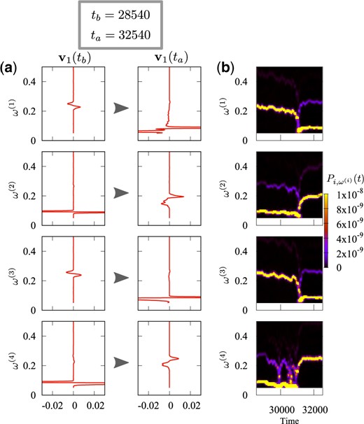
The switching taking place at |$t'=30\,540$| is analyzed in more detail. (a) Comparison of the first eigenvectors before and after the switching, i.e., |$t_{\rm b}=28\,540$| and |$t_{\rm a}=32\,540$|, respectively. (b) Time series of the wavelet spectra |$\left|\tilde p_i\left(\omega,t\right)\right|^2$| for |$i=1,\ldots,N$| around |$t'=30\,540$|. We can see that the wavelet spectra of all of the degrees of freedom exhibit changes.
In Fig. 16, the trajectory is shown in the space |$(p_i,q_i)$| for |$i=1,\ldots,N$| before and after the switching at |$t'=30\,540$|. The figures in the left column show the plot before the switching, i.e., the points from |$t=29\,540$| to |$t=30\,540$|; those in the right column show that after the switching, i.e., the points from |$t=30\,540$| to |$t=31\,540$|. There, we can see that all of the four degrees of freedom are involved in the switching. This would be a characteristic feature of a system with interaction involving multiple degrees of freedom like the Froeschlé map with |$N=4$|. This result suggests that we can extract those features indicating which degrees of freedom are dynamically active from further analysis of the time variation of the eigenvectors.
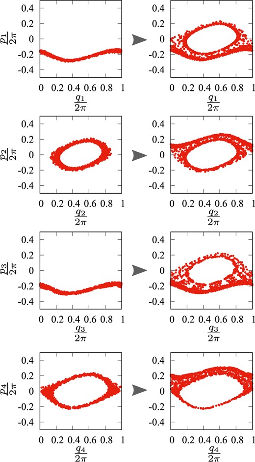
The trajectory is shown in the space |$(p_i,q_i)$| for |$i=1,\ldots,N$| before and after the switching |$t'=30\,540$|. The figures in the left column show the plot before the switching, i.e., the points from |$t=29\,540$| to |$t=30\,540$|; those in the right column show that after the switching, i.e., the points from |$t=30\,540$| to |$t=31\,540$|.
In Fig. 17, we show time series of the local frequencies defined by |$\omega^{(i)}(t')=\mathop{\rm arg~max}\limits_{\omega_l}\left|v_{j=(i,l)}^{(1)}(t')\right|$| for |$i=1,\ldots,N$| plotted on the frequency planes |$(\omega^{(i)},\omega^{(j)})$| for pairs |$(i,j)$| for |$i,j=1,\ldots,N$|. Dots with different colors indicate that they belong to those regions of time separated by the switching at |$t'=30\,540$| detected in Fig. 14(c). These figures indicate which degrees of freedom show a modest variation in their oscillatory motion and which exhibit a violent one. While clusters in the local frequencies show modest variation for those degrees of freedom, scattered dots indicate those that exhibit violent changes. Thus, the switching detected by our method has corresponding features in Fig. 17. These results suggest that we could extract information concerning nonlinear resonances among multiple degrees of freedom by WlPCA. Such analysis would shed some light on the structure of the Arnold web in systems of multiple degrees of freedom.
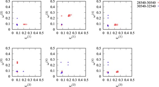
Time series of the local frequencies defined by |$\omega^{(i)}(t')=\mathop{\rm arg~max}\limits_{\omega_l}\left|v_{j=(i,l)}^{(1)}(t')\right|$| for |$i=1,\ldots,N$| plotted on the frequency planes |$(\omega^{(i)},\omega^{(j)})$| for pairs |$(i,j)$| for |$i,j=1,\ldots,N$|. Dots with different colors indicate that they belong to those regions of time separated by the switching at |$t'=30\,540$| detected in Fig. 14(c).
6. Conclusions and future prospects
We have proposed a new method called wavelet local PCA (WlPCA) to analyze trajectories for systems of many degrees of freedom. By combining the wavelet transformation and local PCA in time, our method reduces the dimensionality of time series both in degrees of freedom and frequency so that characteristic features of oscillatory motion can be captured. In particular, local analysis in time enables us to extract nonstationary aspects of the oscillatory behavior. We have applied our method to the Froeschlé maps of |$N=2$| and |$N=4$|, which correspond to autonomous systems of three and five degrees of freedom, respectively.
We have shown that vibrational motions of the models exhibit both relatively stationary features and switching among them. Using WlPCA, we can detect those times when frequency variations exhibit switching between these quasi-stationary oscillations. Moreover, analysis of eigenvectors obtained by WlPCA makes it possible to see which degrees of freedom and frequencies are involved in the switching. We have confirmed that these switchings actually correspond to the onset of transport processes between confined movements in the phase space. These findings suggest that, even for systems of larger degrees of freedom, the phase space is divided into multiple regions where trajectories are confined within them for a finite time. Thus, our analysis indicates that the method is promising for time series analysis toward systems of many degrees of freedom. In particular, the method would be useful to investigate the mechanism of vibrational energy redistribution in molecules.
The essence of our method lies in the following two aspects: (i) locality in time and (ii) dimensional reduction. The former is common in other methods for analyzing phase space such as local Lyapunov analysis [21] and frequency mapping [24]. Both of these methods are shown to be effective for extracting the Arnold web for systems of three degrees of freedom. However, no application of them has been tried for systems of even larger degrees of freedom, since we cannot visualize their results for such systems. Therefore, combining these methods with dimensional reduction is inevitable for such applications. As for the local Lyapunov analysis, dimensional reduction could be done when we analyze not only local Lyapunov exponents but also their corresponding Lyapunov vectors, though the Lyapunov vectors reveal only the linearized motions around the orbits. Then, our method and the local Lyapunov analysis thus extended can be considered as complementary. The former pays attention to the oscillatory features of the dynamics, the latter to the hyperbolic ones.
We can further develop our method in the following directions. First, we are planning to apply WlPCA to systems of even larger degrees of freedom. Understanding chaotic behavior for systems of many degrees of freedom has been hampered because of the difficulty of visualizing trajectories for them. We expect that WlPCA will provide us with a useful method to study these systems. Second, we will characterize the various features exhibited by the eigenvectors obtained by WlPCA, such as the number of degrees of freedom that are involved in the switching. Such features would be valuable in answering the following questions: How does the number of degrees of freedom involved in the switching change in time? How often are specific degrees of freedom involved in the switching? Are there any degrees of freedom that are active participants of the switching? Third, we can resort to the theory of random matrices to analyze statistical properties of avoided crossings and the distribution of the eigenvalues. Such an application has already been done in the study of ergodicity [57], financial data [75], and entanglement in quantum chaos [76] to see any deviation from the prediction of random matrices. A similar analysis would be possible to investigate avoided crossings obtained in WlPCA to extract any features that deviate from the prediction of statistical physics. Fourth, we can extend our method so that we can extract other features of the times series. For example, we can replace PCA with canonical correlation analysis (CCA) to obtain wavelet local CCA. We can also replace the wavelet transformation with other over-complete bases using the sparse way [67], so that we can analyze nonlinear waveforms that appear in times series of, e.g., the brain wave. Fifth, we aim to make our algorithm to find switching automatic so that we can detect switching as fast as possible. Sixth, we should note that the application of WlPCA is not limited to Hamiltonian dynamics, since the wavelet transformation and dimensional reduction are universal in data mining. Therefore, it can also be applied to time series of dissipative dynamics and those obtained by experiments. These developments will be pursued in the near future.
Acknowledgements
K.F. would like to thank Prof. S. Kitsunezaki for suggesting the idea to detect switching shown in Fig. 6. This work has been supported by the Cooperative Research Program of the Network Joint Research Center for Materials and Devices, the Dynamic Alliance for Open Innovation Bridging Human, Environment and Materials, Grants-in-Aid for Challenging Exploratory Research (No. 22654047 and No. 25610105 to M.T.) from Japan Society for the Promotion of Science (JSPS), Grants-in-Aid for Scientific Research (C) (No. 24540394, No. 26400421, and No. 19K03653 to M.T.) from Japan Society for the Promotion of Science (JSPS), and Nara Women’s University Intramural Grant for Project Research (to M.T.).
