


Abstract
Based on Kreimer’s method [Z. Phys. C 54, 667 (1992) and Int. J. Mod. Phys. A 8, 1797 (1993)], we present analytic results for scalar one-loop four-point Feynman integrals with complex internal masses. The results are not only valid for complex internal masses, but also for real internal mass cases. Unlike the traditional approach proposed by ’t Hooft and Veltman [Nucl. Phys. B 153, 365 (1979)], this method can be extended to evaluate tensor integrals directly. Therefore, it may provide a new approach to solve the inverse Gram determinant problem analytically. We then implement the results into a computer package, ONELOOP4PT.CPP. In numerical checks, we compare the program to LoopTools version|$2.12$| in both real and complex mass cases. We find a perfect agreement between the results generated from this work and LoopTools.
1. Introduction
Future colliders, like the Large Hadron Collider (LHC) at high luminosities and the International Linear Collider (ILC) [1–3], aim to measure the properties of the Higgs boson (or to explore the Higgs sector) of top quark and vector bosons, as well as search for physics beyond the standard model (BSM). These measurements will be performed at high precision, e.g., the Higgs boson couplings will be measured at a precision of |$1\%$| or better for a statistically significant measurement [3]. In order to match the high-precision data in the near future, higher-order corrections from theoretical calculations are necessary. Therefore, detailed evaluations of one-loop multi-leg and higher-loop on a general scale to the selected scattering cross sections at the colliders are urgently required.
In the traditional framework, the cross section of the processes at one-loop corrections will be obtained by integrating over the phase space of squared amplitudes, which are decomposed into tensor integrals. These tensor ones are then reduced into scalar one-loop one-, two-, three-, and four-point functions. It is well known that the traditional tensor reductions may meet the inverse Gram determinant problem [4,5] at several kinematic points in the phase space. Consequently, this leads to numerical instabilities. One may apply suitable experimental cuts to avoid the problem. However, the situation is completely different when we consider one-loop multi-leg processes, for instance, |$2\rightarrow 5,6,$| etc., where the higher-point functions will be reduced to scalar one-loop one-, two-, three-, and four-point functions with arbitrary configurations. As a result, we cannot avoid the inverse Gram determinant problem as in the former case. So far, the problem has not been solved analytically and completely.
In the calculation of electroweak corrections to multi-particle processes, we have to handle one-loop integrals with arbitrary internal mass and external momentum assignments. Moreover, for such processes involving unstable particles that can be on-shell, one has to resume their propagators by introducing complex masses [6]. Therefore, the evaluations for tensor and scalar one-loop integrals on a general scale, with complex internal masses, are also important.
The calculations for scalar one-loop one-, two-, three-, and four-point functions are important ingredients for evaluating higher-order corrections. A pioneering calculation for these functions was performed by ’t Hooft and Veltman [7]. For the one-, two-, and three-point functions, the authors of Ref. [7] provided compact explicit expressions that are valid for real and complex internal masses as well as on a general scale. For the scalar four-point functions, an analytic result for real mass cases was presented in Refs. [7,8]. However, only complex mass cases were discussed in these papers. Recently, Ref. [9] has extended the method of ’t Hooft and Veltman for computing scalar one-loop four-point functions with complex internal masses. It has already been implemented into a FORTRAN program, called D|$0$|C. In addition, the authors of Ref. [10] have followed the previous work of Refs. [7,8] for evaluating these functions with complex internal masses in which all infrared (IR) divergence cases have been treated completely.
In addition to these works, it is worth mentioning Refs. [14–19]. In general statements, these calculations for scalar one-loop Feynman integrals follow the traditional approach developed by ’t Hooft and Veltman. The alternative methods that we mention in this paper are presented in Refs. [20,21]. In these papers, the methods have only been developed for evaluating one-loop corrections to quantum chromodynamics (QCD) processes.
Based on the above methods, there are many computer packages available, such as those presented in Refs. [14,22,24–28]. To our knowledge, these calculations and packages have still not solved the inverse Gram determinant problem analytically and completely. Besides that, some of them have still not provided scalar one-loop integrals for complex masses.
The direct computation method (DCM), which is a purely numerical method, has been applied to evaluate Feynman integrals. The method is based on a combination of an efficient numerical integration and extrapolation [33]. Scalar one-loop integrals for real/complex masses have been calculated successfully in this approach. Another purely numerical program, SecDec [29–32], is based on the sector decomposition method. Numerical Mellin–Barnes representations for Feynman integrals have also been presented in Ref. [34].
Solving the Gram determinant problem analytically and proving an alternative method for evaluating scalar one-loop Feynman integrals, in particular for four-point functions, including complex internal masses, are both essential. In the scope of this paper, based on the method developed in Refs. [11–13], we present analytic results for scalar one-loop four-point Feynman integrals with complex internal masses. The results are not only valid for complex internal masses, but also for real mass cases. Unlike the method proposed by G. ’t Hooft and M. Veltman in Ref. [7], this method can be extended to evaluate tensor integrals directly. Therefore, it may provide a new approach to solve the inverse Gram determinant analytically. We then implement the results into a computer package, ONELOOP4PT.CPP. In numerical checks, we compare this work to LoopTools version |$2.12$| [22] in both the real and complex mass cases. We find a perfect agreement between the results generated from this work and LoopTools.
The layout of the paper is as follows. In Sect. 2, we present the method for evaluating scalar one-loop four-point functions in detail. In Sect. 3, we will show the numerical checks on the program with LoopTools. Conclusions and plans for future work are presented in Sect. 4. Several useful formulae used in this calculation are shown in the appendix.
2. The calculation
The term |$i\rho$| is Feynman’s prescription. |$p_i$| and |$m_i$| for |$i =1,2,3,4$| are external momenta and internal masses respectively. The external momenta flow inwards as shown in Fig. 1 and follow the momentum conservation law |$p_1 +p_2 +p_3+ p_4=0$|. The loop momentum is |$l$| and |$n$| is the space-time dimension. In this calculation, we are not going to deal with infrared divergence. Thus, we will work directly in the space-time dimension |$n=4$|. In general, |$D_0$| is a function of |$p_1^2, p_2^2, p_3^2, p_4^2, s, t, m_1^2, m_2^2, m_3^2, m_4^2$| with |$s= (p_1+p_2)^2$|, |$t= (p_2+p_3)^2$|.
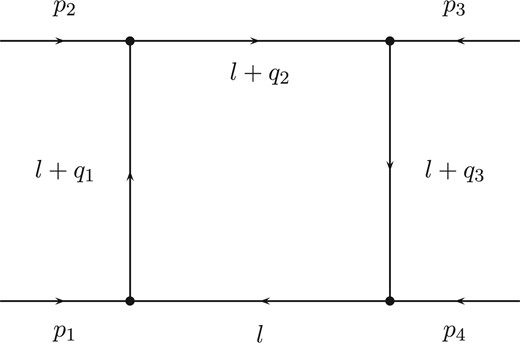
The box diagrams.
It is important to note that the kinematic variables |$a_{lk}, b_{lk}, c_{lk} \in \mathbb{R}$| and |$ d_{lk}\in \mathbb{C}$|. In the following subsections, we are going to calculate this integral.
2.1. Linearization and |$l_0$|-integration
We realize that |$\mathrm{Im}\left(\dfrac{z^2+y^2+t^2+m_k^2-i \rho}{2z} \right) =- \dfrac{m_{0k} \Gamma_{k} +\rho}{2z}$|, which depends on the sign of |$z$|. The location of |$x_0$| in the |$x$|-complex plane will be determined by the sign of |$z$|; see Fig. 2 for more details. We should therefore rewrite |$D_0$| as follows:
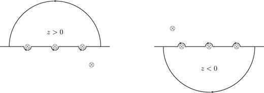
The contour integration in the |$x$|-plane.
2.2. The |$y$|-integration
We are now going to evaluate the threefold integrals introduced in the previous subsection; see Eqs. (25) and (26). In order to work out the |$y$|-integration, one has to linearize |$y$| by using the Euler shift |$t\rightarrow t+y$|. However, we realize that the terms proportional to |$t^2$| and |$y^2$| in the integrand have the same sign. One can first make |$t^2$| and |$y^2$| have opposite signs by applying a complex rotation in the |$t$|-plane.
Because of Eq. (32), we find that |$t_{1,2}$| are located in the first and third quarters of the |$t$|-complex plane, as described in Fig. 3. Because of this, one should choose the integration contour on the fourth quarter of the |$t$|-complex plane, as in Fig. 3. There are no residua of |$t$|-poles that contribute to the |$t$|-integration contour. We therefore derive the following relation:
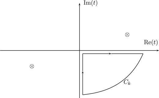
|$t$|-rotation.
We note that |$D_{mlk}\in \mathbb{R}$| and |$F_{nmlk}\in \mathbb{C}$|.
We have just arrived at the twofold integrations. In the following subsections, we will present the approach to calculating these integrals (51)–(54) in detail.
2.3. The |$t$|-integration
The relations between |$D_{mlk}$| and the external momenta are shown in Table 1.
|$D_{mlk}$| given in terms of external momenta.
| |$l=1,k=2$| | |$q_1-q_2=-p_2$| | |$D_{m12}=-4\frac{p_2^2}{AC_{lk}^2}$| |
| |$l=1,k=3$| | |$q_1-q_3=-p_2-p_3$| | |$D_{m13}=-4\frac{(p_2+p_3)^2}{AC_{lk}^2}$| |
| |$l=1,k=4$| | |$q_1-q_4=p_1$| | |$D_{m14}=-4\frac{p_1^2}{AC_{lk}^2}$| |
| |$l=2,k=3$| | |$q_2-q_3=-p_3$| | |$D_{m23}=-4\frac{p_3^2}{AC_{lk}^2}$| |
| |$l=2,k=4$| | |$q_2-q_4=p_1+p_2$| | |$D_{m24}=-4\frac{(p_1+p_2)^2}{AC_{lk}^2}$| |
| |$l=3,k=4$| | |$q_3-q_4=-p_4$| | |$D_{m34}=-4\frac{p_4^2}{AC_{lk}^2} $| |
To follow the calculation easily, we would like to omit the index for the kinematic variables that appear in Eq. (62) in the rest of this paper.
2.3.1. In the case of |$D_{mlk} <0$|
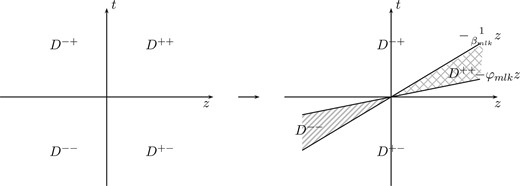
In this case, |$\beta_{mlk} \leqslant 0$| and |$\varphi_{mlk}\geqslant 0$|. The integration region now looks like Fig. 4.
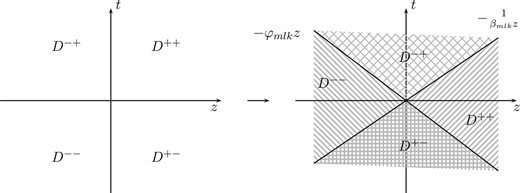
The integration region.
These integrals are calculated in concrete terms in the appendix.
2.3.2. In the case of |$0<D_{mlk}\leqslant \left(\frac{A_{mlk}}{B_{mlk}}-\alpha_{lk}\right)^2$| and |$\frac{A_{mlk}}{B_{mlk}}-\alpha_{lk} < 0$|
It is easy to check that |$-\varphi_{mlk}-(-\frac{1}{\beta_{mlk}}) = -\sqrt{\left(\frac{A_{mlk}}{B_{mlk}}-\alpha_{lk}\right)^2-D_{mlk}}\leqslant0$|. Therefore, the integration region now looks like Fig. 5. In this case, the integration region of |$D_0$| is similar to the |$D_{mlk}<0$| case. As a result, the analytical calculation of |$D_0$| in this case is the same as that in the case of |$D_{mlk}<0$|.
The integration region.
2.3.3. In the case of |$0<D_{mlk}\leqslant \left(\frac{A_{mlk}}{B_{mlk}}-\alpha_{lk}\right)^2$| and |$\frac{A_{mlk}}{B_{mlk}}-\alpha_{lk}> 0$|
Therefore, the integration region now looks like Fig. 6.
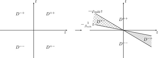
The integration region.
The last integrals written in terms of |$z$| will be evaluated by means of the basic integrals presented in the appendix.
2.3.4. In the case of |$D_{mlk} > \left(\frac{A_{mlk}}{B_{mlk}}-\alpha_{lk}\right)^2$|
We have already added to |$D_0$| the extra terms, the sum of which is up to zero. These extra terms will contribute to the residue of the |$z$|-poles when |$\beta_{mlk}, \varphi_{mlk}$| become complex.
2.3.5. In the case of |$D_{mlk}=0$|
The remaining integrals (written in terms of |$t$|) will be integrated by using the basic integrals, which are described in the appendix.
The traditional tensor reduction for one-loop integrals was proposed by Passarino and Veltman [4] and later developed by Denner and Dittmaier [5]. In these schemes, the form factors will be obtained by contracting the Minkowski metric (|$g_{\mu\nu}$|) and external momenta into the tensor integrals. At this stage, we have to solve a system of linear equations where the Gram determinants appear in the denominator. If the Gram determinants vanish or become very small, the reduction method will break or spoil the numerical stability (this is called the Gram determinant problem). The framework in this paper can be extended to calculate the form factors (or tensor one-loop integrals) directly. This will be the subject of a future publication (K. H. Phan, manuscript in preparation). It therefore provides a new approach to solve the Gram determinant problem analytically.
3. Numerical checks
In this section, we are going to check the program with LoopTools version |$2.12$| [22] (called LoopTools v.|$2.12$|). In Tables 2 and 3, we check ONELOOP4PT.CPP with LoopTools in real and complex masses respectively. The input parameters are presented in these tables. One finds a good agreement between this work and LoopTools in all cases.
In the case of |$(m_1^2,m_2^2,m_3^2,m_4^2)=(10, 20,30,40)$|, and |$ \rho=10^{-30}.$|
| |$(p_1^{2}, p_2^2, p_3^2, p_4^2, s, t)\;$| | This work LoopTools v.|$2.12$| |
|---|---|
| |$(10,50,10,70, 170, 10)$| | |$-1.221\,979\,771\,717\,3585\times 10^{-4}+2.009\,833\,708\,713\,9847\times 10^{-3}\; i$| |
| |$-1.221\,979\,769\,699\,2298\times 10^{-4}+2.009\,833\,709\,284\,3695\times 10^{-3}\; i$| | |
| |$(10,50,10,70, 170, -10)$| | |$-1.486\,716\,266\,289\,6689\times 10^{-4}+1.697\,624\,355\,415\,6623\times 10^{-3}\; i$| |
| |$-1.486\,716\,266\,482\,8184\times 10^{-4}+1.697\,624\,355\,242\,6918\times 10^{-3}\;i$| | |
| |$(10,-50,10,-70, 170, 10)$| | |$\;\;\;3.351\,965\,931\,200\,3411\times10^{-4} + 2.912\,362\,010\,029\,4989\times 10^{-4}\; i$| |
| |$\;\;\;3.351\,965\,931\,227\,0943\times 10^{-4} + 2.912\,362\,011\,787\,9053\times 10^{-4}\; i$| |
In the case of |$m_1^2=10-5i,m_2^2=20-2i, m_3^2=30-3i, m_4^2=40-4i$|, and |$ \rho=10^{-30}.$|
| |$(p_1^{2}, p_2^2, p_3^2, p_4^2, s, t)$| | (This work) |$\times 10^{-4}$| (LoopTools v.|$2.12$|)|$\times 10^{-4}$| |
|---|---|
| |$(10,60,10,90,200,10)$| | |$-7.675\,495\,827\,590\,1917+ 7.936\,923\,630\,833\,591\,22\; i$| |
| |$ -7.675\,495\,827\,590\,2069+ 7.936\,923\,630\,833\,577\,94\; i $| | |
| |$(10,60,-10,90,200,10)$| | |$ -6.221\,361\,528\,827\,8696+ 8.202\,897\,883\,235\,273\,71\; i$| |
| |$ -6.221\,361\,528\,827\,8837 + 8.202\,897\,883\,235\,259\,00\; i$| | |
| |$(10,-60,-10,-90,200,-10)$| | |$\;\;\;1.531\,845\,524\,366\,8001 + 2.561\,867\,870\,169\,164\,87\; i$| |
| |$\;\;\;1.531\,845\,524\,366\,7963 + 2.561\,867\,870\,169\,158\,70\; i$| | |
| |$(10,60,0,0,200,-10)$| | |$-3.349\,931\,574\,662\,3337 + 6.178\,621\,892\,720\,976\,45\; i$| |
| |$-3.349\,931\,574\,662\,3217 + 6.178\,621\,892\,720\,981\,60\; i$| |
In Table 4, we compare the results generated by ONELOOP4PT.CPP with LoopTools by changing the value of |$m_3^2$|. The other input parameters are fixed as follows: |$(p_1^{2}, p_2^2, p_3^2, p_4^2, s, t)=(10, -60,-10,-90,200,-10)$| and |$(m_1^2,m_2^2,m_4^2)=(10-5i,20-2i,40-4i)$|, and |$ \rho=10^{-30}.$| One again finds a good agreement between the results computed from this work and LoopTools in all cases of |$m_3^2$|.
In the case of |$(p_1^{2}, p_2^2, p_3^2, p_4^2, s, t)=(10, -60,-10,-90,200,-10)$| and |$(m_1^2,m_2^2,m_4^2)=(10-5i,20-2i,40-4i)$|, and |$ \rho=10^{-30}.$|
| |$m_3^{2}$| | This work LoopTools v.|$2.12$| |
|---|---|
| |$10-3i$| | |$ 2.225\,160\,881\,981\,8614\times 10^{-4}+3.603\,281\,499\,379\,6746\times 10^{-4}\; i$| |
| |$2.225\,160\,881\,981\,8662\times 10^{-4}+3.603\,281\,499\,379\,6724\times 10^{-4}\; i$| | |
| |$100-3i$| | |$ 8.345\,421\,685\,133\,3892\times 10^{-5}+1.392\,861\,635\,442\,8907\times 10^{-4}\; i$| |
| |$ 8.345\,421\,685\,133\,4176\times 10^{-5}+1.392\,861\,635\,442\,8922\times 10^{-4}\; i$| | |
| |$1000 -3i$| | |$1.558\,129\,882\,600\,2613\times 10^{-5}+2.240\,482\,177\,961\,2569\times 10^{-5}\; i$| |
| |$1.558\,129\,882\,600\,2624\times 10^{-5}+2.240\,482\,177\,961\,2618\times 10^{-5}\;i$| | |
| |$100\,000 -3i$| | |$1.830\,817\,081\,036\,1346\times 10^{-6}+2.415\,245\,966\,391\,0780\times 10^{-6}\; i$| |
| |$1.830\,817\,081\,036\,1369\times 10^{-6}+2.415\,245\,966\,391\,0805\times 10^{-6}\; i$| |
4. Conclusions
In this paper, we have presented the analytic solution for scalar one-loop four-point integrals with real and complex internal masses. This method can be extended to calculate tensor integrals directly. It may provide a new way to solve the inverse determinant problem analytically. In the numerical checks, we compared this work with LoopTools. We found a good agreement between the results generated from this work and those from LoopTools. In future work, we will use this method to evaluate tensor one-loop four-point integrals.
Acknowledgements
This research is funded by the Vietnam National Foundation for Science and Technology Development (NAFOSTED) under grant number 103.01-2016.33. The author is also grateful to Chau Thien Nhan for reading the manuscript and to all members of the Theoretical Physics Department, University of Science Ho Chi Minh City for fruitful discussions. K. H. Phan is grateful to Dr Do Hoang Son for fruitful discussions and his contribution to this work.
Funding
Open Access funding: SCOAP|$^3$|.
Appendix

The integration contour.
We consider three basic integrals in the following paragraphs.
- |$\underline{\mathrm{Basic\,\,\,integral}\,I:}$|: The basic integral |$I$| is defined aswith |$x,y\in \mathbb{C}$|.(A9)
- |$\underline{\mathrm{Basic\,\,\,integral}\,II:}$|: The basic integral |$II$| iswith |$r, x,y\in \mathbb{C}$|.(A10)
- |$\underline{\mathrm{Basic\,\,\,integral}\,III:}$|: The basic integral |$III$| has the formwith |$G(z)$| and |$S(\sigma,z) $| being defined in Eqs. (79) and (87) respectively. We know that |$\text{Im} \left(\frac{ S(\sigma,z)}{Pz+Q}\right)$| is independent of |$\sigma$|; we can then expand the integrand as(A11)where |$A_0, B_0, C_0$| are given by(A12)(A13)(A14)(A15)For |$ \text{Im}\Bigg(\dfrac{ S(\sigma,z)}{Pz_0+Q}\Bigg) \geq 0$| in the region |$\Omega \subset \mathbb{R}$|, one then has
The integral on the right-hand side of this equation can be reduced to basic integral |$I$|.
