Abstract
A recently proposed new mechanism of |$D$|-term-triggered dynamical supersymmetry breaking is reviewed. Supersymmetry is dynamically broken by a nonvanishing |$D$|-term vacuum expectation value, which is realized as a nontrivial solution of the gap equation in the self-consistent approximation, as in the case of the Nambu–Jona-Lasinio model and BCS superconductivity.
1. Introduction
Supersymmetry (SUSY) is an attractive solution to the hierarchy problem, but it has to be broken spontaneously at low energy because of undiscovered superparticles. SUSY should be broken nonperturbatively or dynamically [1, 2] according to the nonrenormalization theorem [3]. Although the mechanism of dynamical SUSY breaking (DSB) by the |$F$|-term has been much explored [4–8], models of DSB by the |$D$|-term were not known. Several years ago, a simple mechanism of |$D$|-term DSB (DDSB) was proposed by H. Itoyama and the present author [9–11], in which the nonvanishing vacuum expectation value (VEV) of the |$D$|-term is dynamically realized as a nontrivial solution of the gap equation in the self-consistent Hartree–Fock approximation, as in the case of the Nambu–Jona-Lasinio (NJL) model [12, 13] and BCS superconductivity [14, 15]. In our mechanism, the gauge sector is extended to be |$\mathcal {N} = 2$| supersymmetric, and the gaugino becomes massive by the |$D$|-term VEV through the Dirac mass term with an |$\mathcal {N}=2$| partner fermion for the gaugino. Thus, our mechanism can be directly applied to the Dirac gaugino scenario [16], which is an interesting alternative extension of the minimal SUSY Standard Model (MSSM). Much attention has been paid to various phenomenological studies based on the Dirac gaugino scenario and its extensions [17–54].
This paper is organized as follows. In the next section, we start out by exhibiting the component action from that of the superspace and state the set of assumptions that we have made. We review the original reasoning that led us to |$D$|-term-triggered DSB. We set up the background field formalism to be used in the subsequent sections, separating the three kinds of background from the fluctuations. In Sect. 3, we elaborate upon our treatment of the effective potential with the three kinds of background fields as well as the point of the Hartree–Fock approximation in Refs. [9–11]. Section 4 is the main thrust of this paper. We present our variational analyses of the effective potential in full detail. Treating one of the order parameters, the |$F$|-term, as an induced perturbation, we demonstrate that the stationary values of the |$D$|-term and an adjoint scalar field are determined by the intersection of the two real curves, namely, the simultaneous solution to the gap equation and the equation of stationarity for the adjoint scalar field. Numerical analysis is provided that demonstrates the existence of such a solution as well as the self-consistency of our analysis. The second variation of the scalar potential is computed and the local stability of the vacuum is shown from the numerical data. Section 5 will discuss the lifetime of our SUSY-breaking vacuum. Unlike the non-SUSY case, our SUSY-breaking vacuum is necessarily metastable because of the positive semidefiniteness of the vacuum energy in the rigid SUSY theory. Namely, the vacuum energy of our SUSY-breaking vacuum is higher than the SUSY vacuum, which is a trivial solution of the gap equation. We will show that the lifetime of our vacuum can be sufficiently large by adjusting the parameters in the theory. In Sect. 6, a realization of the observed Higgs mass by extra |$U(1)$||$D$|-term contributions to the Higgs mass will be discussed [55]. A summary is given in the last section.
2. The action, assumptions, and some properties
The action we discuss is the general
|$\mathcal {N}=1$| supersymmetric action consisting of a chiral superfield
|$\Phi ^a=\big (\phi ^a, \psi ^a, F^a\big )$| in the adjoint representation and a vector superfield
|$V^a=\big (\lambda ^a, V_\mu ^a, D^a\big )$| with three input functions, the Kähler potential
|$K\big (\Phi ^a, \bar {\Phi }^a\big )$| with its gauging, the gauge kinetic superfield
|$\tau _{ab}\big (\Phi ^a\big )$| that follows from the second derivatives of a generic holomorphic function
|$\mathcal {F}\big (\Phi ^a\big )$|, and the superpotential
|$W\big (\Phi ^a\big )$|:
The gauge group is taken to be
|$U(N)$| and, for simplicity, we assume that the theory is in the unbroken phase of the entire gauge group, which can be accomplished by tuning the superpotential. We also assume that third derivatives of
|$\mathcal {F}\big (\Phi ^a\big )$| at the scalar vacuum expectation values (VEVs) are nonvanishing.
The component Lagrangian of Eq. (
1) reads
where
where
and
|$f_{ac}^b$| is the structure constant of
|$SU(N)$|. Note that the equation of motion for
|$F^a$| is
|$F^a = -g^{ab} \overline {\partial _bW}$| + fermions. We also assume
|$\big \langle F^a \big \rangle _{{\rm tree}} = - \big \langle g^{ab} \overline {\partial _b W} \big \rangle _{{\rm tree}} =0$| at tree level. At the lowest order in perturbation theory, there is no source that gives a VEV to the auxiliary field
|$D^0$|:
|$\big \langle D^0 \big \rangle _{{\rm tree}} = 0$|. The
|$U(N)$| gaugino is massless at tree level while the fermionic partner of the scalar gluon receives the tree-level mass
|$m_a = m_0 = \Big \langle g^{00} \partial _0 \partial _0 W \Big \rangle _{{\rm tree}} $|.
2.1. Original reasoning of DDSB
In Ref. [9], it was shown that the VEV of an auxiliary field |$D^0$| is nonvanishing in the Hartree–Fock approximation. Therefore, the theory realizes |$D$|-term dynamical supersymmetry breaking.
The part of the Lagrangian providing the fermion mass matrix of size
|$2N$| is
It was observed that the auxiliary
|$D^a$| field, which is an order parameter of
|$\mathcal {N} =1$| supersymmetry, couples to the fermionic (but not bosonic) bilinears through the third prepotential derivatives: the nonvanishing VEV of
|$D^0$| immediately gives the Dirac mass of the fermions. The equation of motion for the auxiliary field
|$D^0$| implies
telling us that the condensation of the Dirac bilinear is responsible for
|$\big \langle D^0 \big \rangle \neq 0$|. This feature reminds us of the electromagnetic
|$U(1)$| symmetry breaking in BCS theory by Cooper-pair condensation or the chiral symmetry breaking in quantum chromodynamics by quark–antiquark condensation.
We diagonalize the holomorphic part of the mass matrix:
Note that the nonvanishing third prepotential derivatives are
|$\mathcal {F}_{0aa}$|, where
|$a$| refers to the generators of the unbroken gauge group. By an orthogonal transformation, we obtain the two eigenvalues of Eq. (
9) for each generator, which are of mixed Majorana–Dirac type:
Introducing
we obtain
It was also shown in Ref. [
9] that the nonvanishing
|$F^0$| term is induced by the consistency of our procedure of computation (see also Refs. [
56,
57]). This is because the stationary value of the scalar fields gets shifted upon the variation (the vacuum condition). The final mass formula for the
|$SU(N)$| fermions is to be read off from
We will write down the explicit form in the next subsection; see Eqs. (
15), (
16), (
17), and (
18). One of the main points remaining is how to establish the procedure in which the stationary values of the scalar fields,
|$D^0$| and
|$F^0$|, perturbatively induced, are determined, which we will resolve in this paper.
2.2. Quadratic part of the quantum action
In this subsection, we write down the parts of the action with background fields for the computation of the one-loop determinant in the next section.
2.2.1. Fermionic part
Let us extract the fermion bilinears from Eqs. (
3), (
4), and (
5), which are needed for our analysis in what follows. Rescaling the fermion fields so that their kinetic terms become canonical, we obtain
Here the fermion fields
|$\psi ^a$|,
|$\bar {\psi }^a$|,
|$\lambda ^a$|,
|$\bar {\lambda }^a$| are to be integrated to make a part of the effective potential, while the gauge kinetic function
|$\mathcal {F}_{aa}$|, the Kähler metric
|$g_{aa}$|, and their derivatives are functions of the
|$U(N)$| singlet
|$c$|-number background scalar field
|$\varphi ^0$|. The order parameters of supersymmetry
|$F^0$|,
|$\bar {F}^0$|, and
|$D^0$| are taken as background fields as well.
From the Lagrangian
|$\mathcal {L}_F$|, the holomorphic part of the mass matrix is read off as
We parametrize this matrix such that, in the case of
|$F^0=\bar {F}^0=0$|, its form reduces to that of Refs. [
9,
10]. The quantities with multiple indices such as
|$\mathcal {F}_{0aa}$| receive
|$U(N)$|-invariant expectation values:
|$\big \langle \mathcal {F}_{0aa} \big \rangle = \big \langle \mathcal {F}_{000} \big \rangle $| etc. We suppress the indices as we work with the unbroken
|$U(N)$| phase in this paper:
The two eigenvalues of the holomorphic mass matrix are written as
where
These provide the masses for the two species of
|$SU(N)$| fermions once the stationary values are determined.
2.2.2. Bosonic part
Next, we extract the bosonic quantum bilinears from Eqs. (
3), (
4), and (
5). Let
where
|$\varphi ^0$| are the background fields while
|$\tilde {\varphi }^a$|,
|$\tilde {A}_\mu ^a$|,
|$\tilde {F}^a$|, and
|$\tilde {D}^a$| are the quantum scalar, vector, and auxiliary fields, respectively.
We obtain
We have also ignored
|$-\frac {1}{8}({\rm Re}~\mathcal {F})_{ab}\epsilon ^{\mu \nu \rho \sigma }F_{\mu \nu }^a F_{\rho \sigma }^b$| as we eventually set
|$\varphi ^a$| constant in our analysis and this term becomes a total derivative.
2.3. Connection with previous work
We stop briefly here to address the connection of Ref. [9] with the previous work. Models of dynamical supersymmetry breaking with nonvanishing |$F$|- and |$D$|-terms have been previously proposed; for instance, the 3–2 model [6] and the 4–1 model in Ref. [56]. In these models, the supersymmetry is unbroken at tree level and is broken by the nonvanishing VEV of the |$F$|-term through instanton-generated superpotentials. The nonvanishing VEV of the |$D$|-term is also induced, but is much smaller than that of the |$F$|-term.
In our mechanism, the supersymmetry is unbroken at tree level, and is broken in a self-consistent Hartree–Fock approximation of NJL type that produces a nonvanishing VEV for the |$D$|-term. A nonvanishing VEV for the |$F$|-term is induced in our Hartree–Fock vacuum that shifts the tree vacuum and we explore the region of the parameter space in which the |$F$|-term VEV is treated perturbatively.
We should mention that the way in which the two kinds of gauginos (or the gaugino and the adjoint matter fermion) receive masses is an extension of that proposed in Ref. [16]: a pure Dirac-type gaugino mass is generated in Ref. [16] while a mixed Majorana–Dirac-type gaugino mass is generated in our case, the Majorana part being given by the second derivative of the superpotential. In Ref. [16], the dynamical origin of the nonvanishing |$D$|-term VEV was not addressed.
As for the application to dynamical chiral symmetry breaking, a supersymmetric NJL-type model has been considered [58–61]. Chiral symmetry is not spontaneously broken in a supersymmetric case. Even in softly broken supersymmetric theories, the chiral symmetry broken phases are degenerate with the chirally symmetric ones. Thus, in supersymmetric theories, the phase with broken chiral symmetry is no longer the energetically preferred ground state.
3. The effective potential in the Hartree–Fock approximation
The goal of this section is to determine the effective potential to the leading order in the Hartree–Fock approximation. We will regulate the one-loop integral by dimensional reduction [62]. We prepare a supersymmetric counterterm, and set the normalization condition. We make brief comments on regularization and subtraction schemes at the end of Sect. 4. We also change the notation for expectation values in general from |$\langle \cdots \rangle $| to |$\cdots _*$|, as the main thrust of this paper is the determination of the stationary values from the variational analysis.
In the Hartree–Fock approximation, one begins with considering the situation where one-loop corrections in the original expansion in |$\hbar $| become large and are comparable to the tree-level contribution. The optimal configuration of the effective potential to this order is found by matching the tree against the one-loop, varying with respect to the auxiliary fields. We start an analysis of this kind for our effective potential. There are three constant background fields as arguments of the effective potential: |$\varphi \equiv \varphi ^0~({\rm complex})$|, |$U(N)$|-invariant background scalar, |$D \equiv D^0~({\rm real})$|, and |$F \equiv F^0~({\rm complex})$|. The latter two are the order parameters of |$\mathcal {N}=1$| supersymmetry.
We vary our effective potential with respect to all these constant fields and examine the stationary conditions. We also examine a second derivative at the stationary point along the constraints of the auxiliary fields to understand better the Hartree–Fock corrected mass of the scalar gluons. Let us denote our effective potential by
|$V$|. It consists of three parts:
The first term is the tree contributions, the second one is the counterterm, and the last one is the one-loop contributions. After the elimination of the auxiliary fields, the effective potential is referred to as the scalar potential so as to be distinguished from the original
|$V$|.
3.1. The tree part
To begin with, let us write down the tree part and find a parametrization by two complex and one real parameters. We also introduce the simplifying notation
|$g_{00}\big (\varphi , \bar {\varphi }\big ) \equiv g\big (\varphi , \bar {\varphi }\big ), ({\rm Im}\,\mathcal {F}(\varphi ))_{00} \equiv {\rm Im}\,\mathcal {F}''(\varphi ), \partial _0 W(\varphi ) = W'(\varphi ), g_{00,0} \equiv \partial g,$| etc:
As a warm-up, let us determine the vacuum configuration by a set of stationary conditions at tree level:
Equation (
26) determines the stationary value of
|$D$|:
while from Eq. (
27) we obtain
Equation (
28) together with these two gives
as well as
The negative coefficients of the RHS of Eq. (
25) imply that both the
|$D$| and
|$F$| profiles of the potential have a maximum for a given
|$\varphi $|. These signs are, of course, the right signs for the stability of the scalar potential, as is clear by completing the square. This is a trivial comment to make here but will become less trivial later. The mass of the scalar gluons at tree level
|$\big |m_{s*}\big |^2$| is read off from the second derivative at the stationary point:
As we have already introduced in Eq. (
16),
|$\Delta $| and
|$r$| are defined by
Recall that we have suppressed the indices, invoking the
|$U(N)$| invariance of the expectation values. Also,
where
|$f_3$| differs from
|$f$| in Eq. (
16) by
We obtain
We also see that the mass scales of the problem are set by
|$m_{s*}$|, the scalar gluon mass, and
|$g^{-1} \overline {\mathcal {F}}'''_*$|, the third prepotential derivative (and
|$g^{-1} \partial g$|), once the stationary value of the scalar is determined.
3.2. Treatment of UV infinity
In the NJL theory [
12,
13], there is only one coupling constant carrying dimension
|$-1$| and the dimensionless quantity is naturally formed by combining it with the relativistic cutoff, which is interpreted as the onset of UV physics. In the theory with which we are concerned, UV physics is specified by three input functions,
|$K, \mathcal {F}, W$|, and the UV scales and infinities reside in some of the coefficients. Our supersymmetric counterterm [
9,
10] is
This is a counterterm associated with
|${\rm Im}\mathcal {F}''$|. We set up a renormalization condition
and relate (or transmute) the original infinity of the dimensional reduction scheme with that of
|${\rm Im}\,\mathcal {F}''$|. We have indicated that this condition is set up at
|$D=0$| and the stationary point of the scalar that we will determine. We stress again that the entire scheme is supersymmetric.
3.3. The one-loop part
The entire contribution of all particles in the theory to
|$i \cdot $| (the one particle irreducible to one-loop)
|$\equiv i \Gamma _{1-{\rm loop}}$| is easy to compute, knowing (
17), (
18), and (
34). It is given by
In the unbroken
|$U(N)$| phase, it is legitimate to replace
|$\displaystyle \sum _a$| by
|$N^2$| and drop the index
|$a$|, as we have said before. We obtain
Note that the
|$\big |m_s\big |^2$|, whose stationary values give the tree mass squared of the scalar gluon, differ from
|$|{\rm tr}\mathcal {M}|^2$|:
To evaluate the integral in
|$d$| dimensions, we just quote
where
We obtain
This again depends upon
|$\Delta $|,
|$f$|, and
|$\varphi $|.
4. Stationary conditions and gap equation
4.1. Variational analyses
Now we turn to our variational problem. It is stated as in the tree case as
We will regard the solution to be obtained by considering Eqs. (
49) and (
51) first and solving
|$D$| and
|$\varphi $| for
|$F$| and
|$\bar {F}$|:
Equation (
50) is then
and its complex conjugate. These will determine
|$F=F_*, \bar {F}=\bar {F}_*$|.
In this paper, we are going to work in the region where the magnitude
|$\left | F_* \right |$| is small and can be treated perturbatively. This means that, in the leading order, the problem posed by Eq. (
49) and Eq. (
51) becomes
Equation (
54) is nothing but the gap equation given in Refs. [
9,
10], while Eq. (
55) is the stationary conditions for the scalar. This is the variational problem that we should solve. A set of stationary values
|$\big (D_*, \varphi _*, \bar {\varphi }_*\big )$| is determined as the solution.
4.2. The analysis in the region |$F_* \approx 0$|
Let us first determine
|$V(D, \varphi , \bar {\varphi }, F=0, \bar {F}=0)$| explicitly. We need to solve the normalization condition:
where
|$J$| has been introduced in Eq. (
43). At
|$F, \bar {F} \to 0$|,
where
essentially reducing the situation to that of Refs. [
9,
10].
Note, however, that
|$r$| and
|$\Delta ({\rm or} \ r_0, \Delta _0)$| are complex in general, except for those special cases that include the case of the rigid
|$\mathcal {N}=2$| supersymmetry partially broken to
|$\mathcal {N}=1$| at the tree vacua. For
|$|\Delta _0| \ll 1$|,
We solve the normalization condition for the number
|$A$| to obtain
We obtain
After some calculation, this is found to be expressible as
where
Note that
and
If
|$r_0$| (and
|$\Delta _0$|) is real, this is rewritten as
where
|$c' \equiv \frac {c}{r_{0*}^2 \big |m_{s*}\big |^4}$| is the rescaled number, and
Clearly, there are two scales in our current problem
|$|r_{0*}|^{-1/2}$| and
|$\big |m_{s*}\big |$|, which are controlled by the second superpotential derivative and the third prepotential derivative at the stationary value
|$\varphi _*$|.
Let us turn to the gap equation
For Eq. (
64), scaling out
|$|r_0|^2$|, we find
where
Note that
|$|1-\cos 2(\theta -\theta ')| \to 0$| in the region
|$\theta \sim 0$| or
|$|\Delta _0| \gg 1$|.
On the other hand, for Eq. (
70) with
|$\Delta _0$| being real,
|$N^2 \big |m_s\big |^4$| is scaled out and it is simply given by the
|$\Delta _0$| derivative:
which is our original gap equation.
1 In both cases, the solutions are given by the extremum of the potential
|$V_0(D, \varphi , \bar {\varphi })$| in its
|$D$| profile. We stress again that the
|$D$| profile is not a direct stability criterion of the vacua, which is to be discussed with regard to the scalar potential
|$V_0\Big (D_*\big (\varphi , \bar {\varphi }\big ), \varphi , \bar {\varphi }\Big )$|.
We next examine
|$\left . \frac {\partial V_0}{\partial \varphi } \right |_{D, \bar {\varphi }}=0$| and its complex conjugate. For Eq. (
64), we obtain
and its complex conjugate where
The second term of the RHS of Eq. (
76) is proportional to the gap equation (
73). As for the third term, after some calculation, we obtain
In the RHS of Eqs. (
76) and (
78), we have regarded
|$\Delta _0$|,
|$\bar {\Delta }_0$|,
|$\varphi $|, and
|$\bar {\varphi }$| as independent variables.
For Eq. (
70), with
|$\Delta _0$| real, we obtain
and its complex conjugate. Here, in the last term of the RHS, we have regarded
|$\Delta _0$|,
|$\varphi $|,
|$\bar {\varphi }$| as independent variables.
Finally, the stationary values (
|$D_*, \varphi _*, \bar {\varphi }_*$|) are determined by Eqs. (
73) and (
76) in one case or by Eqs. (
75) and (
79) in the other case. Let us discuss the latter case of Eqs. (
75) and (
79) first. As the second term of the RHS in Eq. (
79) is nothing but the gap equation (
75), Eq. (
79) can be safely replaced by
|$\varphi $| being real. The solution to Eq. (
80) in the
|$\Delta _0$| profile is determined as the point of intersection of the potential with the quadratic term having
|$\varphi =\bar {\varphi }$| dependent coefficients. Actually, it is a real curve in the full (
|$\Delta _0, \varphi =\bar {\varphi }$|) plane. Likewise, the solution to the gap equation (
75), the condition of the
|$\Delta _0$| extremum of the potential, provides us with another real curve in the (
|$\Delta _0, \varphi =\bar {\varphi }$|) plane. The values (
|$\Delta _{0*}, \varphi _*=\bar {\varphi }_*$|) are the intersection of these two. A schematic figure of the intersection is displayed in Fig.
1. By tuning our original input functions, it is possible to arrange such intersection. Conversely, as an inverse problem, for given
|$\Delta _{0*}$| and the height of the
|$\Delta _0$| profile, one can always find the values of the coefficients in Eq. (
75) and the coefficient function in Eq. (
80) that accomplish this. Dynamical supersymmetry breaking has been realized.
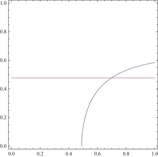
Fig. 1.
A schematic picture of the intersection of the two curves that represent the solution to the gap equation (red) and the |$\varphi $| flat condition (blue). The horizontal axis is denoted by |$\varphi /M$| and the vertical one by |$\Delta _0$|. The values at the stationary point (|$\Delta _{0*}, \varphi _*=\bar {\varphi }_*$|) are read off from the intersection point.
As in the case of Eqs. (
75) and (
79), in the former case of Eqs. (
73) and (
76) we can safely replace Eq. (
76) by
The values (
|$\Delta _{0*}, \bar {\Delta }_{0*}, \varphi _*, \bar {\varphi }_*$|) can be determined by the intersection of Eq. (
73) and Eq. (
81). We will not carry out the (numerical) analysis for this case further in this paper.
4.3. Determination of |$F_*$|
Let us now turn to the analysis of the remaining equation of our variational problem, Eq. (
50). In our current treatment,
As the stationary values
|$\big (D_*, \varphi _*, \bar {\varphi }_*\big )$| are already determined, this equation and its complex conjugate determine
|$F_*$| and
|$\bar {F}_*$|:
Note that, knowing
|$V_{{\rm 1-loop}}$| explicitly in Eq. (
48), the RHS can be evaluated. We can check the consistency of our treatment through
|$f_3$| in Eq. (
36) by
|$|f_3| \ll 1$|.
4.4. Numerical study of the gap equation
In this subsection, we study some numerical solutions to the gap equation (
75) and the stationary condition for
|$\varphi $| (Eq. (
80)) in the real
|$\Delta _0$| case. The equations we should study are
where we note that
|$\delta \big (\varphi , \bar {\varphi }\big )$| in the gap equation (
75) vanishes at the stationary point in the real
|$\Delta _0$| case. By using Eqs. (
70) and (
71), the second condition can be rewritten after dividing by
|$\Delta _{0*}^2$| as
The nontrivial solution
|$\Delta _{0*} \ne 0$| to the gap equation (
84) is found in some region of the parameters
|$c'$| and
|$\tilde {A}$|, which has already been done in Ref. [
9]. This solution fixes the LHS of Eq. (
86) and
|$\varphi _*$| is determined by solving Eq. (
86) in principle. In order to find
|$\varphi _*$| explicitly, the form of the prepotential
|$\mathcal {F}$| and that of the superpotential
|$W$| must be specified. Here, we take a simple prepotential and a superpotential of the following type:
where
|$c, d$| are dimensionless constants while
|$m, M$| are dimensionful parameters. In particular,
|$M$| is a cutoff scale of the theory. This prepotential is minimal for DDSB. As for the superpotential, at least two terms are required to be supersymmetric at tree level. We can take a quadratic term
|$\varphi ^2$| instead of the cubic one, but in that case, the RHS of Eq. (
86) becomes singular because of
|$\partial \ln |m_s|^2=0$|.
Substituting these
|$\mathcal {F}$| and
|$W$| into Eq. (
86), we obtain
where we have utilized the fact that
|$1/M, d, \varphi _*$| are real and
|$c$| is pure imaginary, which are necessary for
|$\Delta _0=\bar {\Delta }_0$|. Taking the coefficients
|$c=i, d=1$| for further simplification, we can easily obtain a solution by tuning
|$N$| and
|${\rm Im}\Lambda $|. We note that
|$0 \le \varphi _*/M \le 1$| for our effective theory to be valid. In the analysis carried out in this paper, we consider the region where the magnitude of the
|$F$|-term is smaller compared to that of the
|$D$|-term. Therefore, we need to check whether our solutions satisfy this property consistently. Let us consider the ratio of the auxiliary fields:
where the form of the prepotential and that of the superpotential in Eq. (
87) and Eq. (
88) are assumed and we have put
|$c=i, d=1$| in the second equality.
Now, the numerical solutions to the gap equation and the stationary condition for |$\varphi $| are listed in Table 1. In these examples, we have taken some values of |$-\frac {N^2}{{\rm Im}(i + \Lambda )}$| and |$m$| just for an illustration and the ratio |$|F_*/D_*|$| and |$|f_{3*}|$| are evaluated. We can find that the |$F$|-term is smaller than the |$D$|-term in some of these examples.
Table 1.Samples of numerical solutions for the gap equation and the stationary condition for |$\varphi $|. The ratio |$|F_*/D_*|$| and |$|f_{3*}|$| are also evaluated for a consistency check.
| |$c'+\dfrac {1}{64\pi ^2}$|
. | |$\left .\tilde {A}\right /\big (4\cdot 32\pi ^2\big )$|
. | |$\Delta _{0*}$|
. | |$\varphi _*\Big /M \left (-\dfrac {N^2}{{\rm Im}(i+\Lambda )}\right )$|
. | |$\big |F_*/D_*\big |$|
. | |$\big |f_{3*}\big |$|
. |
|---|
| 0.002 | 0.0001 | 0.477 | 0.707 (10 000) | 2.621 (|$m=M$|) | 1.77 |
| 0.002 | 0.0001 | 0.477 | 0.707 (10 000) | 0.524 (|$m \ll M$|) | 0.35 |
| 0.002 | 0.0001 | 0.477 | 0.707 (10 000) | 0.860 (|$m=0.4M$|) | 0.58 |
| 0.003 | 0.001 | 1.3623 | 0.8639 (2000) | 0.825 (|$m=M$|) | |$>$|1 |
| 0.003 | 0.001 | 1.3623 | 0.8639 (2000) | 0.224 (|$m \ll M$|) | 0.43 |
| 0.003 | 0.001 | 1.3623 | 0.5464 (5000) | 1.092 (|$m=M$|) | |$>$|1 |
| 0.003 | 0.001 | 1.3623 | 0.5464 (5000) | 0.142 (|$m \ll M$|) | 0.27 |
| 0.003 | 0.001 | 1.3623 | 0.5464 (5000) | 0.911 (|$m=0.9M$|) | 1.76 |
| 0.003 | 0.001 | 1.3623 | 0.3863 (10 000) | 1.444 (|$m=M$|) | |$>$|1 |
| 0.003 | 0.001 | 1.3623 | 0.3863 (10 000) | 0.100 (|$m \ll M$|) | 0.19 |
| 0.003 | 0.001 | 1.3623 | 0.3863 (10 000) | 0.960 (|$m=0.8M$|) | 1.85 |
4.5. Mass of the scalar gluons2
We now turn to the question of the second variations of the scalar potential
at the stationary point (
|$D_*\big (\varphi _*,\bar {\varphi }_*\big ), 0, 0, \varphi _*, \bar {\varphi }_*$|) . It is convenient to separate
|$V\big (D, F, \bar {F}, \varphi , \bar {\varphi }\big )$| into two parts:
Here
and
In Eq. (
93), we have extracted the
|$F, \bar {F}$| dependence of
|$V_{{\rm 1-loop}}$| (Eq. (
48)) and
|$_*$| indicates that they are evaluated at
|$\big (D_*, \varphi _*, \bar {\varphi }_*, 0, 0\big )$| after the derivatives are taken. Equation (
94) has been computed in Eq. (
63) and Eq. (
70). We will compute the second partial derivatives and the second variations of
|$V_{{\rm scalar}}$|.
For
|$\mathcal {V}$|,
|$\vec {y}_L = \big (F, \bar {F}\big ), \vec {y}_R=\big (\varphi , \bar {\varphi }\big )$|,
We obtain, after some computation,
where
We see that, in the region
|$\Big |\big (\partial _F \partial _{\bar {F}} V\big )_0\Big |_*, \Big |\big (\partial _F^2 V\big )_0\Big |_*, \ll g_*$|, the matrix
|$\mathcal {M}_*$| is well approximated by
The two eigenvalues are
respectively, ensuring the positivity of (
99).
For
|$V_0$|,
|$y_L =D, \vec {y}_R=\big (\varphi , \bar {\varphi }\big )$|,
We know that the
|$D$| profile of
|$V_0(D, \varphi , \bar {\varphi })$| near the stationary point is convex to the top and we fit this by
Here
|$\alpha $| is a positive real function of
|$\varphi , \bar {\varphi }$| and
|$V_h\big (\varphi , \bar {\varphi }\big ) = V_0(D_*\big (\varphi , \bar {\varphi }\big ), \varphi , \bar {\varphi })$|. One can check that
while
and
The entire contribution of the second variation
|$\delta ^2 V_* = \delta ^2 \mathcal {V}_* + \delta ^2 V_{0*}$| to the leading order in the Hartree–Fock approximation is given by Eqs. (
99) and (
109). The mass of the scalar gluons squared is obtained by multiplying the combined mass matrix by
|$g^{-1}_*$|:
generalizing the tree formula. In practice, we just need a well approximated formula valid in the region we work with and one can invoke the
|$U(1)$| invariance to ensure that the two eigenvalues of the complex scalar gluons are degenerate. Let us, therefore, use the expression
to check the local stability of the potential and the mass. The above expression is obtained for our simple example of
|$\mathcal {F}$| and
|$W$|,
and the real case
|$\Delta _0=\bar {\Delta }_0$| is applied. Using the numerical analyses carried out in the last subsection, we have made a list of data on Eq. (
111). Except for the last case in Table
2, the scalar gluon masses squared are found to be positive for any
|$N$|, which implies that our stationary points are locally stable. Even in the last case, the stability is ensured for small
|$N$|. In these data, we have checked that the inequalities
|$\big |\big (\partial _F \partial _{\bar {F}} V_{{\rm 1-loop}}\big )\big |_*, \big |\big (\partial _F^2 V_{{\rm 1-loop}}\big )\big |_* \ll g_*$| are in fact satisfied. As a summary of our understanding, a schematic figure is drawn in Fig.
2, which illustrates the local stability of the scalar potential at the vacuum of dynamically broken supersymmetry in comparison with the well known NJL potential.
Table 2.Samples of numerical values for the scalar gluon masses.
| |$c'+\dfrac {1}{64\pi ^2}$|
. | |$\tilde {A}\Big /\Big (4\cdot 32\pi ^2\Big )$|
. | |$\Delta _{0*}$|
. | |$\varphi _*\Big /M \ \left (-\dfrac {N^2}{{\rm Im}(i+\Lambda )}\right )$|
. | Scalar gluon mass
. |
|---|
| 0.002 | 0.0001 | 0.477 | 0.707 (10 000) | 0.4998 + 0.0056 |$N^2$| + |$8.607 \times 10^{-7} N^4$| |
| 0.003 | 0.001 | 1.3623 | 0.8639 (2000) | 0.7463 + 0.0106 |$N^2$| + |$2.653 \times 10^{-4} N^4$| |
| 0.003 | 0.001 | 1.3623 | 0.5464 (5000) | 0.2986 + 0.0008 |$N^2$| + |$4.694 \times 10^{-5} N^4$| |
| 0.003 | 0.001 | 1.3623 | 0.3863 (10 000) | 0.1492 |$-$| 0.0024 |$N^2$| +|$7.235 \times 10^{-5} N^4$| |
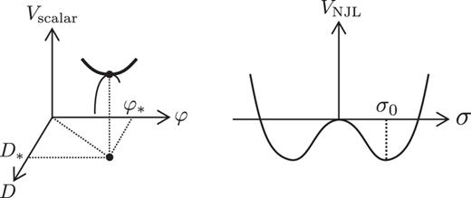
Fig. 2.
Comparison of |$V_{{\rm scalar}}$| around the stationary value |$\big (D_*, \varphi _*\big )$| with |$V_{{\rm NJL}}$|.
4.6. Choice of regularization and subtraction scheme
In this paper, we have considered the theory specified by the general |$\mathcal {N}=1$| supersymmetric Lagrangian Eq. (1), have regularized the theory by supersymmetric dimensional regularization (dimensional reduction), and have subtracted part of the |$1/\epsilon $| poles of the regularized one-loop effective action in Eq. (48) by the supersymmetric subtraction scheme defined by the condition Eq. (40). The original infinity is transmuted into the infinite constant |$\Lambda $|, which is the coefficient of the counter term, and the effective potential has been recast to describe the behavior of the theory well below the UV cutoff residing in the prepotential function.
We now make brief comments on other regularizations and subtraction schemes that we have not employed in this paper. The relativistic momentum cutoff is a natural choice of the NJL theory, as we mentioned earlier, but regularizing the integral Eq. (41) by the momentum cutoff leads us to a rather unwieldy expression; see Ref. [10]. Unlike supersymmetric dimensional reduction [62], the momentum cutoff per se, while preserving the equality between the Bose and Fermi degrees of freedom, does not have a firm basis on the regularized action on which the supersymmetry algebra acts. Moreover, as is clear from (A.1) of Ref. [10], the result violates the positivity of the effective potential in the vicinity of the origin in the |$\Delta $| profile. This violation is a necessity in the broken chiral symmetry of the NJL theory but here it contradicts the positive semidefiniteness of energy that the rigid supersymmetric theory possesses. Turning to the choice of subtraction scheme, one might also like to apply the “(modified) minimal subtraction scheme” in our one-loop integral Eq. (48). While we do not know how to justify this prescription here, the subsequent analyses proceed in almost the same way and the main features of the equations obtained from our variational analyses and the conclusions are unchanged.
5. Lifetime of the metastable SUSY-breaking vacuum
Combining the two facts that the trivial solution
|$\Delta _0=0$| of the gap equation is also a trivial solution and the energy in rigid SUSY theories is positive semidefinite leads us to our SUSY-breaking vacuum being a local minimum. For our mechanism to be viable, we have to show that our SUSY-breaking vacuum is sufficiently long-lived during the decay into the true vacuum with
|$\Delta _0=0$|; in other words, the lifetime of our vacuum must be much longer than the age of the universe. Taking into account the nonvanishing
|$F$|-term VEV induced by the
|$D$|-term VEV as well, we carry out an order estimate of the lifetime of our SUSY-breaking vacuum. Neglecting
|$\mathcal {O}(1)$| quantities, we have
where
|$\Lambda $| is a cutoff scale. Plugging these VEVs into Eq. (4.1) in Ref. [
10],
leads to
provided that
|$m_s \ll \Lambda $|.
The decay rate of our vacuum to the true one is controlled by the factor
|$\exp \big [ - \big |\big \langle \Delta \phi \big \rangle |^4/ \big \langle \Delta V \big \rangle \big ]$|, as seen in Ref. [
64], where
|$\langle \Delta \phi \rangle , \langle \Delta V \rangle $| are the scalar field distance and the potential height between two vacua. These two quantities are estimated as follows:
Using these results, the requirement of the longevity of our metastable vacuum is given by the condition
which is always satisfied as long as
|$m_s \ll \Lambda $|.
6. Higgs mass
In order to realize the observed Higgs mass of 126 GeV in the MSSM, the SUSY-breaking scale should be higher, since the Higgs boson requires large radiative corrections from the top squarks. Also, we have no signals for SUSY particles from the experiments at the Large Hadron Collider (LHC). Thus, the naturalness of the MSSM becomes worse and worse. It is a well known fact that the Higgs mass in the MSSM at tree level is smaller than the |$Z$|-boson mass, but this can be avoided if we consider extensions of the MSSM.
In this section, we investigate the implications of the mechanism of DDSB uncovered in Refs. [
9–11], coupling the system to the MSSM Higgs sector that includes
|$\mu $| and
|$B\mu $| terms [
55]. The pair of Higgs doublet superfields
|$H_u, H_d$| is taken to be charged under the overall
|$U(1)$|:
We have adopted the notation
|$X \cdot Y \equiv \epsilon _{AB} X^A Y^B = X^A Y_A = - Y \cdot X$|,
|$\epsilon _{12} = - \epsilon _{21} = \epsilon ^{21} = - \epsilon ^{12} =1$|.
|$V_{1,2,0}$| are vector superfields of the SM gauge group and that of the overall
|$U(1)$|, respectively, and the corresponding gauge couplings are denoted by
|$g_Y, g_2, e_u$|, and
|$e_d$|, respectively. Unlike the MSSM case, the soft scalar Higgs masses
|$m_{H_u}^2 |H_u|^2, m_{H_d}^2 |H_d|^2$| are not introduced since they are induced by
|$D$|-term contributions in our framework.
To simplify the analysis in what follows while keeping the essence, we adopt the simplest prepotential and superpotential exploited in Eqs. (
87) and (
88) of a
|$5 \times 5$| complex matrix scalar superfield
|$\varphi $|:
where
|$c$| is a pure imaginary number as discussed above, and
|$m,M$| are mass parameters. Here
|$N=5$| and
|$M$| (real number) sets the scale in the prepotential, which is the cutoff scale.
We embed the generators of the gauge group into the bases that expand
|$\varphi $|:
We have represented the overall
|$U(1)$| and
|$U(1)_Y$| generators as being proportional to the unit matrix and the traceless diagonal generator, respectively. We analyze the case in which only
|$S$| receives its VEV, namely, the unbroken
|$U(5)$| vacuum of the superpotential. We will make a comment for those cases in which these do not hold, which lead to kinetic mixing. We drop the octet
|$T_8$| as it is irrelevant to the analysis below.
After a simple calculation, we obtain the nonvanishing prepotential derivatives
their VEVs
and the derivatives of the superpotential
We choose
|$c= 10i$| but
|$\langle S \rangle $| is complex, not necessarily real.
In this paper, we add Eq. (
119) to Eq. (
1) and consider a part relevant to the 126 GeV Higgs:
The third prepotential derivatives, which are now real numbers, can be read off from Eq. (
123).
In our analysis, we assume that the value of the |$D^0$| VEV is determined essentially by our Hartree–Fock approximation in Ref. [11]. This source of supersymmetry breaking is then fed to the Higgs sector and its effects are given by a tree-level analysis. We will argue the validity of this procedure below.
6.1. Higgs potential and variations
Let us extract the part relevant to the Higgs potential in (
125):
where
|$\varphi ^C=(T^a, Y, S)$|. The one-loop part of the effective potential in Refs. [
9,
11] is denoted by
|$\Gamma ^{{\rm 1-loop}}\Big (D^0\Big )$|. Fermionic backgrounds are not needed in the potential analysis of Higgs and are not included in Eq. (
126).
Let us vary
|$\mathcal {L}_{{\rm pot}}$| with respect to the auxiliary fields, replacing
|$\varphi ^C$| by their VEV
|$\Big \langle \varphi ^C \Big \rangle =\big (0, 0, \langle S \rangle \big )$|:
Note that
|$\mathcal {F}_{aa0}=\mathcal {F}_{YY0}=\mathcal {F}_{000} \equiv \mathcal {F}'''$| and that Eq. (
129) with
|$e_u = e_d = 0$| is in fact the gap equation of Refs. [
9,
11]. Eliminating the auxiliary fields (approximately), we obtain the Higgs potential
Here we have denoted by
|$D^{0*}$| the solution to Eq. (
129), the improved gap equation. The deviation
|$\delta D^{0*}$| of the value from
|$D^{0*}$| in Ref. [
11] is in fact small by the ratio of the electroweak and SUSY-breaking scales. Therefore, we approximate the solution to the improved gap equation by the value of
|$D^{0*}$| in Ref. [
11], denoted as
|$\big \langle D^0 \big \rangle $|. Taking into account the fact that
|${\rm Im}\mathcal {F}'''\langle S \rangle \sim \langle S \rangle /M \ll 1$|, we neglect the term
|${\rm Im}\mathcal {F}'''\langle S \rangle $| at the leading order. The resulting Higgs potential at the leading order is given by
where we have restricted the potential to the CP-even neutral sector of Higgs doublets
|$H_u=\big (H_u^+, H_u^0\big )^T$|,
|$H_d=\big (H_d^0, H_d^-\big )^T$| in the second line, since we are interested in the Higgs mass. In the last line, the neutral components of the Higgs fields are parametrized as
where we use the following shorthand notations:
|$G^0$| is the would-be Nambu–Goldstone boson eaten as the longitudinal component of the
|$Z$|-boson. The VEV of the Higgs field is
|$v \simeq 246$| GeV and
|$\frac {g_Y^2+g_2^2}{4}v^2=M_Z^2$| in this convention.
6.2. Estimate of the Higgs mass
We are now ready to calculate the Higgs mass. As in the MSSM, the minimization of the scalar potential
|$\partial V_{{\rm Higgs}}/\partial v^2 = \partial V_{{\rm Higgs}}/\partial \beta = 0$| allows us to express
|$\mu $| and
|$B\mu $| in terms of other parameters:
It is straightforward to obtain the mass matrix for the CP-even Higgs from the second derivative of the potential,
where each component is given by
The eigenvalues of this mass matrix are found as
and the lightet CP-even Higgs mass is
In order for the
|$\mu $|-term to be allowed in the superpotential, we must have a condition
|$e_u+e_d=0$|, which is also required from an anomaly cancellation condition for the overall
|$U(1)$|. Then, the Higgs mass can be expressed as
where
|$\tilde {M}^2_Z \equiv M_Z^2 + e_u^2 v^2$|. It is interesting to see the correspondence between our expression of the Higgs mass (
143) and that in the MSSM:
As in the case of the MSSM, the upper bound of the Higgs mass can be obtained by taking a decoupling limit
|$M_A^2 \to \infty $|:
|$\tilde {M}_Z$| can be large enough by taking
|$\mathcal {O}(1)$| charge
|$e_u$|:
Let us go back to the minimization conditions of the Higgs potential with
|$e_u+e_d=0$|,
which leads to
In order to satisfy this condition, the dominant part in the right-hand side of (
149)
|$e_u \big \langle D^0 \big \rangle /c_{2\beta }$| is required to be negative.
Using these conditions, we can eliminate
|$M_A^2$| in the Higgs mass (
143):
where the approximation
|$\big \langle D^0 \big \rangle \gg \tilde {M}_Z^2$| is applied in the second line.
A plot of the 126 GeV Higgs mass as a function of |$\cos 2\beta $| and |$e_u$| is shown in Fig. 3. Here we have taken |$e_u < 0$| and |$\cos 2\beta >0$| to satisfy the condition |$e_u \big \langle D^0 \big \rangle /c_{2\beta }<0$|. We can immediately see that the 126 GeV Higgs mass is realized by |$\mathcal {O}(1)$| charge |$e_u$|, namely, without fine-tuning of parameters. Also, we found that the result is insensitive to the values of the |$D$|-term VEV. This fact is naturally expected from the nondecoupling nature of the Higgs mass.
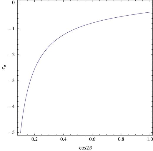
Fig. 3.
A plot of the 126 GeV Higgs mass as a function of |$\cos 2\beta $| and |$e_u$|. The result is insensitive to the values of the |$D$|-term VEV.
7. Summary
In this paper, we have reviewed our recently proposed mechanism of |$D$|-term-triggered dynamical SUSY breaking [9–11, 55]. The nonvanishing |$D$|-term VEV is dynamically realized as a nontrivial solution of the gap equation in the Hartree–Fock approximation, as in the case of the NJL model and BCS superconductivity. In our mechanism, since the gauge sector is extended to be |$\mathcal {N} = 2$| supersymmetric, the gaugino becomes massive by the |$D$|-term VEV through the Dirac mass term with an |$\mathcal {N}=2$| partner fermion for the gaugino. Our mechanism can be directly applied to the Dirac gaugino scenario, which has attracted much attention.
A systematic analysis of the scalar potential was performed by treating the order parameters of SUSY-breaking |$D$| and |$F$|, and the adjoint scalar field as the background fields. It was shown numerically that SUSY is indeed broken dynamically and our metastable vacuum is locally stable. The lifetime of our metastable vacuum was also shown to be sufficiently long-lived.
As a phenomenological application, we have discussed how an observed Higgs mass can be realized in the context of DDSB and have shown that it is naturally realized by an additional overall |$U(1)$||$D$|-term contribution to the Higgs mass.
Acknowledgement
The author would like to thank H. Itoyama for the series of collaborations.
References
1
Witten
E.
,
Nucl. Phys. B
188
,
513
(
1981
).
2
Witten
E.
,
Nucl. Phys. B
202
,
253
(
1982
).
3
Grisaru
M. T.
, Siegel
W.
, and Rocek
M.
,
Nucl. Phys. B
159
,
429
(
1979
).
4
Affleck
I.
, Dine
M.
, and Seiberg
N.
,
Nucl. Phys. B
241
,
493
(
1984
).
5
Affleck
I.
, Dine
M.
, and Seiberg
N.
,
Phys. Lett. B
140
,
59
(
1984
).
6
Affleck
I.
, Dine
M.
, and Seiberg
N.
,
Nucl. Phys. B
256
,
557
(
1985
).
7
Meurice
Y.
and Veneziano
G.
,
Phys. Lett. B
141
,
69
(
1984
).
8
Meurice
Y.
, Veneziano
G.
, Amati
D.
, Konishi
K.
, Meurice
Y.
, Rossi
G. C.
, and Veneziano
G.
,
Phys. Rept.
162
,
169
(
1988
).
9
Itoyama
H.
and Maru
N.
,
Int. J. Mod. Phys. A
27
,
1250159
(
2012
).
10
Itoyama
H.
and Maru
N.
,
Int. J. Mod. Phys. Conf. Ser.
21
,
42
(
2013
). [
] [].
11
Itoyama
H.
and Maru
N.
,
Phys. Rev. D
88
,
025012
(
2013
).
12
Nambu
Y.
and Jona-Lasinio
G.
,
Phys. Rev.
122
,
345
(
1961
).
13
Nambu
Y.
and Jona-Lasinio
G.
,
Phys. Rev.
124
,
246
(
1961
).
14
Bardeen
J.
, Cooper
L. N.
, and Schrieffer
J. R.
,
Phys. Rev.
108
,
1175
(
1957
).
15
Nambu
Y.
,
Phys. Rev.
117
,
648
(
1960
).
16
Fox
P. J.
, Nelson
A. E.
, and Weiner
N.
,
J. High Energy Phys.
0208
,
035
(
2002
).
17
Fayet
P.
,
Phys. Lett. B
78
,
417
(
1978
).
18
Polchinski
J.
and Susskind
L.
,
Phys. Rev. D
26
,
3661
(
1982
).
19
Hall
L. J.
and Randall
L.
,
Nucl. Phys. B
352
,
289
(
1991
).
20
Nelson
A. E.
, Rius
N.
, Sanz
V.
, and Unsal
M.
,
J. High Energy Phys.
0208
,
039
(
2002
).
21
Kribs
G. D.
, Poppitz
E.
, and Weiner
N.
,
Phys. Rev. D
78
,
055010
(
2008
).
22
Benakli
K.
and Goodsell
M. D.
,
Nucl. Phys. B
816
,
185
(
2009
).
23
Benakli
K.
and Goodsell
M. D.
,
Nucl. Phys. B
830
,
315
(
2010
).
24
Benakli
K.
and Goodsell
M. D.
,
Nucl. Phys. B
840
,
1
(
2010
).
25
Benakli
K.
, Goodsell
M. D.
, and Maier
A.-K.
,
Nucl. Phys. B
851
,
445
(
2011
).
26
Benakli
K.
,
Fortschr. Phys.
59
,
1079
(
2011
).
27
Benakli
K.
, Goodsell
M. D.
, and Staub
F.
,
J. High Energy Phys.
1306
,
073
(
2013
).
28
Benakli
K.
, Goodsell
M.
, Staub
F.
, and Porod
W.
,
Phys. Rev. D
90
,
045017
(
2014
).
29
Carpenter
L. M.
,
J. High Energy Phys.
1209
,
102
(
2012
).
30
Choi
S. Y.
, Choudhury
D.
, Freitas
A.
, Kalinowski
J.
, and Zerwas
P. M.
,
Phys. Lett. B
;
698
,
457
(
2011
)
31
Abel
S.
and Goodsell
M.
,
J. High Energy Phys.
1106
,
064
(
2011
).
32
Amigo
S. D. L.
, Blechman
A. E.
, Fox
P. J.
, and Poppitz
E.
,
J. High Energy Phys.
0901
,
018
(
2009
).
33
Fok
R.
and Kribs
G. D.
,
Phys. Rev. D
82
,
035010
(
2010
).
34
Davies
R.
, March-Russell
J.
, and McCullough
M.
,
J. High Energy Phys.
1104
,
108
(
2011
).
35
Kumar
P.
and Ponton
E.
,
J. High Energy Phys.
1111
,
037
(
2011
).
36
Kribs
G. D.
and Martin
A.
,
Phys. Rev. D
85
,
115014
(
2012
).
37
Yan-Min
D.
, Faisel
G.
, Jung
D.-W.
, and Kong
O. C. W.
,
Phys. Rev. D
87
,
085033
(
2013
).
38
Fok
R.
, Kribs
G. D.
, Martin
A.
, and Tsai
Y.
,
Phys. Rev. D
87
,
055018
(
2013
).
39
Frugiuele
C.
, Gregoire
T.
, Kumar
P.
, and Ponton
E.
,
J. High Energy Phys.
1303
,
156
(
2013
).
40
Unwin
J.
,
Phys. Rev. D
86
,
095002
(
2012
).
41
Csaki
C.
, Goodman
J.
, Pavesi
R.
, and Shirman
Y.
,
Phys. Rev. D
89
,
055005
(
2014
).
42
Dudas
E.
, Goodsell
M.
, Heurtier
L.
, and Tziveloglou
P.
,
Nucl. Phys. B
884
,
632
(
2014
).
43
Goodsell
M. D.
and Tziveloglou
P.
,
Nucl. Phys. B
889
,
650
(
2014
).
45
Nelson
A. E.
and Roy
T. S.
,
Phys. Rev. Lett.
114
,
201802
(
2015
).
46
Ding
R.
, Li
T.
, Staub
F.
, Tian
C.
, and Zhu
B.
,
Phys. Rev. D
92
,
015008
(
2015
).
47
Alves
D. S. M.
, Galloway
J.
, Weiner
N.
, and McCullough
M.
, [
] [].
48
Martin
S. P.
,
Phys. Rev. D
92
,
035004
(
2015
).
49
Goodsell
M. D.
, Krauss
M. E.
, Müller
T.
, Porod
W.
, and Staub
F.
,
J. High Energy Phys.
1510
,
132
(
2015
).
50
Chakraborty
S.
, Datta
A.
, Huitu
K.
, Roy
S.
, and Waltari
H.
, [
] [].
51
Ding
R.
, Li
T.
, Staub
F.
, and Zhu
B.
, [
] [].
52
Morita
Y.
, Nakano
H.
, and Shimomura
T.
, [
] [].
53
Nakano
H.
and Yoshikawa
M.
, [
] [].
54
Carpenter
L. M.
, Colburn
R.
, and Goodman
J.
, [
] [].
55
Itoyama
H.
and Maru
N.
,
Symmetry
7
,
193
(
2015
).
56
Dine
M.
, Nelson
A. E.
, Nir
Y.
, and Shirman
Y.
,
Phys. Rev. D
53
,
2658
(
1996
).
57
Carpenter
L. M.
, Fox
P. J.
, and Kaplan
D. E.
, [
] [].
58
Buchmuller
W.
and Love
S. T.
,
Nucl. Phys. B
204
,
213
(
1982
).
59
Clark
T. E.
, Love
S. T.
, and Bardeen
W. A.
,
Phys. Lett. B
237
,
235
(
1990
).
60
de la Macorra
A.
and Ross
G. G.
,
Nucl. Phys. B
404
,
321
(
1993
).
61
Faisel
D.
, Jung
W.
, and Kong
O. C. W.
,
J. High Energy Phys.
1201
,
164
(
2012
).
62
Siegel
W.
,
Phys. Lett. B
84
,
193
(
1979
).
63
Itoyama
H.
and Maru
N.
,
Nucl. Phys. B
893
,
332
(
2015
).
64
Intriligator
K. A.
, Seiberg
N.
, and Shih
D.
,
J. High Energy Phys.
0604
,
021
(
2006
).
© The Author(s) 2016. Published by Oxford University Press on behalf of the Physical Society of Japan.
This is an Open Access article distributed under the terms of the Creative Commons Attribution License (
http://creativecommons.org/licenses/by/4.0/), which permits unrestricted reuse, distribution, and reproduction in any medium, provided the original work is properly cited.Funded by SCOAP
3


