


Abstract
A potential model for the interaction between a charmed baryon (|$\Lambda _c$|, |$\Sigma _c$|, and |$\Sigma _c^*$|) and the nucleon (|$N$|) is constructed. The model contains a long-range meson (|$\pi $| and |$\sigma $|) exchange part and a short-distance quark exchange part. The quark cluster model is used to evaluate the short-range repulsion and a monopole type form factor is introduced to the long-range potential to reflect the extended structure of hadrons. We determine the cutoff parameters in the form factors by fitting the |$NN$| scattering data with the same approach and we obtain four sets of parameters (a)–(d). The most attractive potential (d) leads to bound |$\Lambda _c N$| states with |$J^\pi = 0^+$| and |$1^+$| once the channel couplings among |$\Lambda _c$|, |$\Sigma _c$|, and |$\Sigma _c^*$| are taken into account. One can also investigate many-body problems with the model. Here, we construct an effective |$\Lambda _c N$| one-channel potential with the parameter set (d) and apply it to the three-body |$\Lambda _c NN$| system. The bound states with |$J=1/2$| and |$3/2$| are predicted.
1. Introduction
Recent developments in hadron spectroscopy have revealed that there may exist various molecular bound states of hadrons (observed as hadron resonances). In particular, the observation of the unexpected X, Y, and Z mesons and the ensuing theoretical studies indicate that heavy quark molecules are more plausible. This can be understood from the balance between the kinetic term and the potential in the Hamiltonian: a heavier system has a smaller kinetic energy [1–3].
The above naive expectation motivates us to explore possible bound states composed of charmed (or bottomed) baryons |$Y_{c(b)}$| (|$\Lambda _{c(b)}$|, |$\Sigma _{c(b)}$|, |$\ldots $|) and the nucleon (|$N$|) or nucleus. This is, of course, a natural extension of the hypernucleus, which is a nuclear bound state with one or more strange baryons |$Y(\Lambda $|, |$\Sigma $|, |$\Xi $|, |$\ldots $|). Hypernuclear spectroscopy in recent decades played a key role in analyzing structures of hypernuclei and extracting information on the |$YN$| and |$YY$| interactions. Because there are no two-body bound states in |$\Lambda N$| or |$\Sigma N$| systems and it is difficult to perform direct scattering experiments for the hyperons, it is important to get information on their interactions from the three-body or heavier nucleus with strange baryon(s).
The idea of the charmed hypernucleus is, in fact, old [4–13]. It was pointed out [6–8] that the SU(4) symmetry, though it is badly broken, for the one-boson exchange (OBE) models predicts a weaker attraction between |$Y_c$| and |$N$|, because the |$K$| exchange is replaced by the |$D$| exchange, which is suppressed by the heavier mass of the |$D$| meson. Recent re-analysis with a model based on the heavy quark effective theories suggested the possibility of bound |$Y_c N$| states. However, the model has a difficulty in describing the short-range interaction and its prediction was very sensitive to the cutoff parameters in the one-boson exchange interaction [11].
In this paper, we construct a potential model consisting of the long-range one-pion and one-sigma exchange interaction and the quark exchange effect based on the quark cluster model for the baryon–baryon interaction [14–18]. The latter provides a short-range repulsion between |$Y_c$| and |$N$|. Here, |$Y_c$| represents |$\Lambda _c$|, |$\Sigma _c$|, and |$\Sigma ^*_c$|. The model also contains the off-diagonal components, which couple |$\Lambda _cN$|, |$\Sigma _cN$|, and |$\Sigma ^*_c N$| channels of the same total quantum numbers. By adjusting the meson exchange parameters to reproduce low-energy data of the |$NN$| system, we obtain four sets of the |$Y_cN$| potential.
We solve the coupled channel Schrödinger equation using the Gaussian expansion method (GEM) [19] and obtain |$\Lambda _c N$| bound states. The potential is also applied to the three-body |$\Lambda _c NN$| system. Bound state solutions are found and their properties are analyzed.
The paper is organized as follows. In Sect. 2, we present our model of the |$Y_c N$| potential and explain how to determine the model parameters. In Sect. 3, the two-body |$Y_cN$| systems are analyzed with the obtained potentials and the results are examined. In Sect. 4, we construct an effective one-channel |$\Lambda _c N$| potential model and apply it to the three-body |$\Lambda _cNN$| system. Conclusions are given in Sect. 5.
2. Model of |$Y_{c}N$| interactions
We first consider the two-baryon systems, with isospin |$I=\frac {1}{2}$| and spin-parity |$J^{\pi }=0^{+}$| or |$1^{+}$|. Table 1 shows possible channels contributed by |$\Lambda _{c}N$|, |$\Sigma _{c}N$|, and |$\Sigma _{c}^{*}N$| for each |$J$|. The channels with orbital angular momentum |$L=0$| and 2 will be coupled by tensor force, while those with the same |$L$| are coupled mainly by central force. We solve the coupled channel Schr|$\ddot {{\rm o}}$|dinger equation in a hybrid potential model. The model includes a pion exchange potential and a scalar meson exchange potential for long-range interactions [11] and a short-range repulsive potential coming from the quark exchanges between the baryons [14–17].
The S-wave |$\Lambda _{c}N$| states and the channels coupling to them [11].
| Channels | 1 | 2 | 3 | 4 | 5 | 6 | 7 |
|---|---|---|---|---|---|---|---|
| |$J^{\pi } = 0^{+}$| | |$\Lambda _{c}N({}^{1}S_{0})$| | |$\Sigma _{c}N({}^{1}S_{0})$| | |$\Sigma _{c}^{*}N({}^{5}D_{0})$| | ||||
| |$J^{\pi } = 1^{+}$| | |$\Lambda _{c}N({}^{3}S_{1})$| | |$\Sigma _{c}N({}^{3}S_{1})$| | |$\Sigma _{c}^{*}N({}^{3}S_{1})$| | |$\Lambda _{c}N({}^{3}D_{1})$| | |$\Sigma _{c}N({}^{3}D_{1})$| | |$\Sigma _{c}^{*}N({}^{3}D_{1})$| | |$\Sigma _{c}^{*}N({}^{5}D_{1})$| |
2.1. One-boson exchange potential
2.2. Short-range repulsion from the quark cluster model
In a previous approach [11], we considered exchanges of the vector mesons for the short-range part of the |$Y_{c}N$| interaction. They, however, do not provide enough repulsion at short distances and result in very deep bound states with compact wave functions. As the wave functions of the baryons overlap significantly at short distances, the quark exchange effect becomes important. We employ here the quark cluster model (QCM) for the short-range potential [14–17].
The overall strength |$\beta $| can be determined by the |$\Delta (1232)$|–nucleon |$(N)$| mass splitting, which also comes from |$V_{\rm CM}$|. From |$\left \langle V_{\rm CM} \right \rangle _{\Delta } - \left \langle V_{\rm CM} \right \rangle _{N} = -16 \beta = 293$| MeV (exp.), we obtain |$\beta \cong 18.2$| MeV. Table 2 shows the values of |$V_{\rm CM}$| for various two-baryon (six-quark) states. These values are evaluated in the heavy quark limit, so that the heavy quark spin does not contribute.
Expectation values in MeV of the color–magnetic interaction (CMI) for the relevant channels in the heavy quark limit. For the correlated channels of |$\Sigma _cN$| and |$\Sigma _c^{*}N$|, the values are given in the matrix form.
| System | |$V_{0}$| [MeV] |
|---|---|
| |$(NN)^{S=0}_{I=1}$| | 450 |
| |$(NN)^{S=1}_{I=0}$| | 350 |
| |$(\Lambda _cN)^{S=0}_{I=1/2}$| | 300 |
| |$(\Lambda _cN)^{S=1}_{I=1/2}$| | 300 |
$\left (\begin
{matrix} \Sigma _cN \\ \Sigma _c^{*}N \end
{matrix}\right )^{S=0}_{I=1/2} = \left ( \begin {matrix}
100 & 0 \\ 0 & 0 \end {matrix}\right ), \quad
\left (\begin {matrix} \Sigma _cN \\ \Sigma _c^{*}N \end
{matrix}\right )^{S=1}_{I=1/2} = \left ( \begin {matrix}
166.7 & -24.0 \\ -24.0 & 108.3 \end
{matrix}\right )$ | |
The range parameter |$b$| is supposed to coincide with the extension of the quark wave functions in the baryon. According to [18], typical values for the |$NN$| interaction are about |$0.54 \sim 0.58$| fm. For |$Y_{c}N$| systems, we use two typical values, |$b=0.5$| and |$0.6$| fm, and compute the results.
2.3. Coulomb potential
2.4. Determining the potential parameters
In the previous study using the OBE potential [11], we found that the results are very sensitive to the cutoff parameters. To remedy this problem, in the present approach we adjust the parameters of the potential to reproduce the |$NN$| interaction data using the same model. In doing so, we fix the |$\pi $|-baryon coupling constants and the short-range potential derived from the quark model. Then the cutoffs, |$\Lambda _{\pi }$| and |$\Lambda _{\sigma }$|, and the sigma coupling constant, |$C_{\sigma }$|, are the parameters to be determined in the |$NN$| system. After that the results are generalized to the |$Y_c N$| system. In this method, we assume that the light mesons couple only to the light quarks and the cutoff parameters are common to |$NN$| and |$Y_c N$| systems. The details are given in Appendix B.
The |$NN$| two-body parameters for |$\Lambda _{\pi }=750$| MeV.
| |$b=0.6$| [fm] | |$b=0.5$| [fm] | |||||
|---|---|---|---|---|---|---|
| __________________________ | _________________________ | |||||
| |$\Lambda _{\sigma }$| [MeV] | |$C_{\sigma }(0^{+})$| | |$C_{\sigma }(1^{+})$| | |$\Delta _{C}$| | |$C_{\sigma }(0^{+})$| | |$C_{\sigma }(1^{+})$| | |$\Delta _{C}$| |
| 900 | |$-$|213.16 | |$-$|161.29 | 51.87 | |$-$|176.89 | |$-$|132.25 | 44.64 |
| 950 | |$-$|179.56 | |$-$|134.56 | 45.0 | |$-$|148.84 | |$-$|110.25 | 38.59 |
| 1000 | |$-$|156.25 | |$-$|118.81 | 37.44 | |$-$|129.96 | |$-$|96.04 | 33.92 |
| 1050 | |$-$|141.61 | |$-$|106.09 | 35.52 | |$-$|116.64 | |$-$|86.49 | 30.15 |
| 1100 | |$-$|127.69 | |$-$|96.04 | 31.65 | |$-$|106.09 | |$-$|79.21 | 26.88 |
| 1150 | |$-$|116.64 | |$-$|88.36 | 28.28 | |$-$|98.01 | |$-$|72.25 | 25.76 |
| 1200 | |$-$|108.16 | |$-$|82.81 | 25.35 | |$-$|90.25 | |$-$|67.24 | 23.01 |
The |$NN$| two-body parameters for |$\Lambda _{\sigma }=1000$| MeV.
| |$b=0.6$| [fm] | |$b=0.5$| [fm] | |||||
|---|---|---|---|---|---|---|
| __________________________ | _________________________ | |||||
| |$\Lambda _{\pi }$| [MeV] | |$C_{\sigma }(0^{+})$| | |$C_{\sigma }(1^{+})$| | |$\Delta _{C}$| | |$C_{\sigma }(0^{+})$| | |$C_{\sigma }(1^{+})$| | |$\Delta _{C}$| |
| 500 | |$-$|148.84 | |$-$|139.24 | 9.6 | |$-$|118.81 | |$-$|121.0 | 2.19 |
| 550 | |$-$|151.29 | |$-$|136.89 | 14.4 | |$-$|123.21 | |$-$|116.64 | 6.57 |
| 600 | |$-$|153.76 | |$-$|134.56 | 19.2 | |$-$|125.44 | |$-$|114.49 | 10.95 |
| 650 | |$-$|153.76 | |$-$|129.96 | 23.8 | |$-$|127.69 | |$-$|110.25 | 17.44 |
| 700 | |$-$|156.25 | |$-$|125.44 | 30.81 | |$-$|127.69 | |$-$|104.04 | 23.65 |
| 750 | |$-$|156.25 | |$-$|118.81 | 37.44 | |$-$|129.96 | |$-$|96.04 | 33.92 |
| 800 | |$-$|156.25 | |$-$|110.25 | 48.51 | |$-$|129.96 | |$-$|88.36 | 41.6 |
| 850 | |$-$|156.25 | |$-$|102.01 | 54.24 | |$-$|132.25 | |$-$|79.21 | 53.04 |
| 900 | |$-$|156.25 | |$-$|92.16 | 66.6 | |$-$|132.25 | |$-$|70.56 | 61.69 |
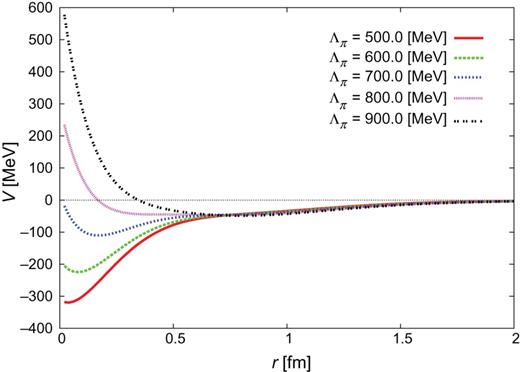
From the results in the tables, one finds that |$\Delta _{C}$| is insensitive changes in |$\Lambda _{\sigma }$|, but |$\Delta _{C}$| increases rapidly for increasing |$\Lambda _{\pi }$|. The features for |$b=0.5$| fm and |$0.6$| fm are qualitatively similar. Since the QCM repulsion for |$b=0.5$| fm is weaker than that for |$b=0.6$| fm, the resulting |$C_{\sigma }$| is also smaller and |$\Delta _{C}$| tends to be smaller for |$b=0.5$| fm. We suppose that the spin dependence of |$C_{\sigma }$| is small, so that a small |$\Delta _{C}$| is favored.
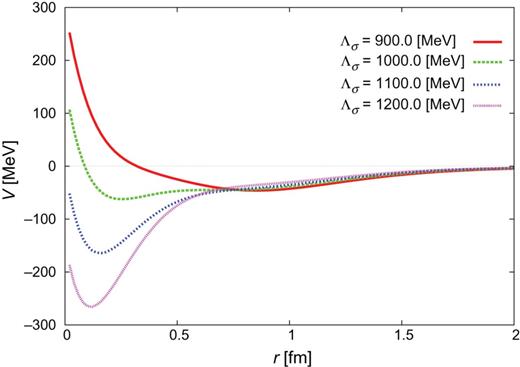
The resulting |$NN$| potentials for |$J^{\pi }=0^{+}$| with the parameters obtained are plotted in Figs. 1 and 2. We find that some of the potentials (for small |$\Lambda _{\pi }$|) are strongly attractive at short distances and may not be appropriate for the current purpose, although they all reproduce the |$^{1}S_{0}$| scattering length and the deuteron binding energy.
|$NN$| potential |$(J^{\pi }=0^{+})$| for |$b=0.6$| fm and |$\Lambda _{\sigma }=1000$| MeV.
|$NN$| potential |$(J^{\pi }=0^{+})$| for |$b=0.6$| fm and |$\Lambda _{\pi }=750$| MeV.
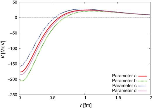
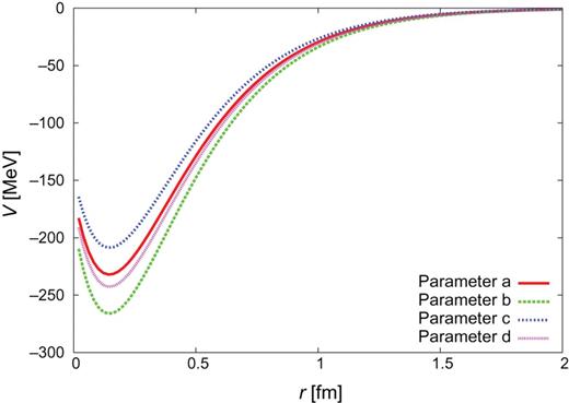
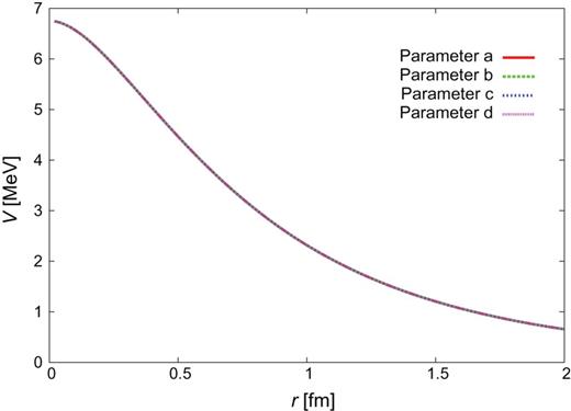
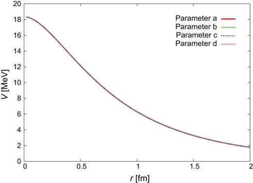
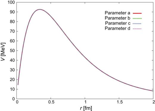
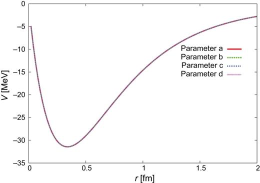
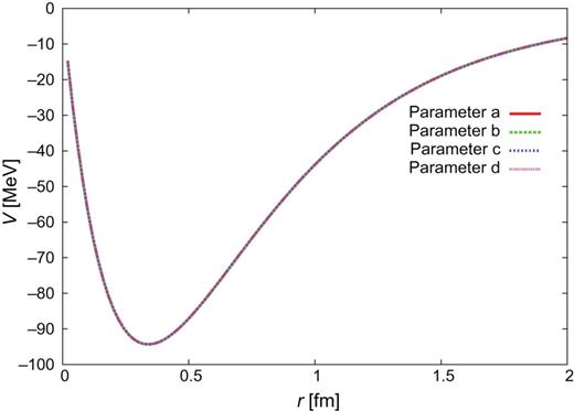
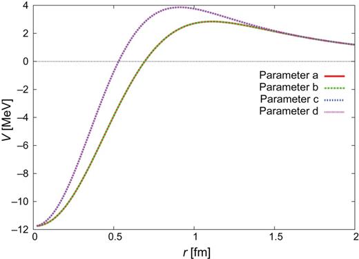
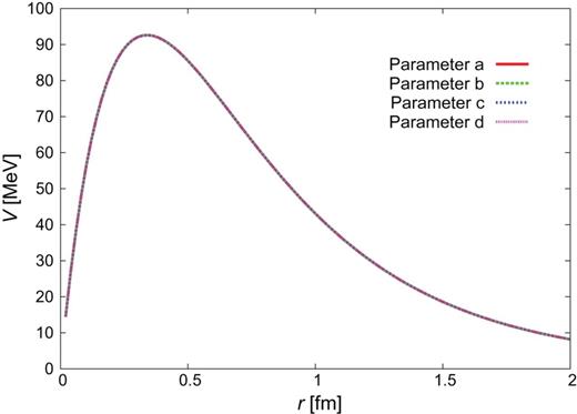
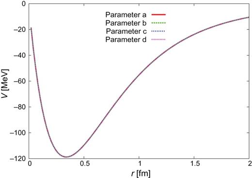
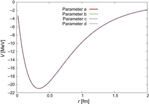
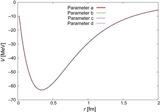
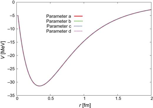
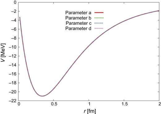
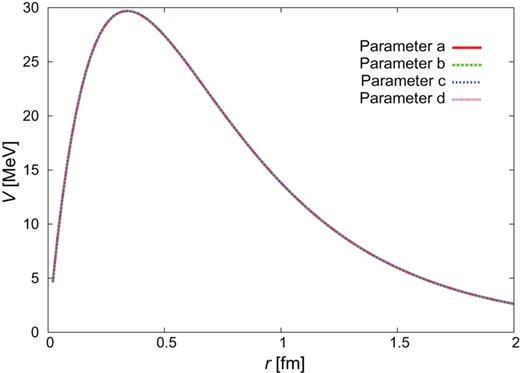
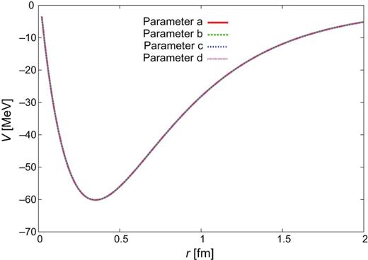
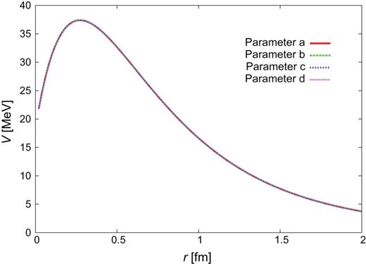
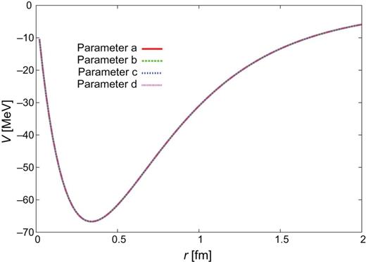
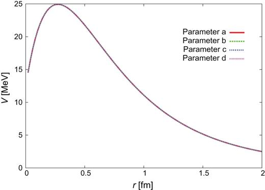
Therefore we choose the parameters with |$\Lambda _{\pi }=750$| MeV and |$\Lambda _{\sigma }=1000$| MeV, and employ four sets of the most realistic potential parameters, given in Table 5. We call these models “CTNN” potentials, as these parameter sets correspond to the |$NN$| experimental data. The |$Y_{c}N$| potentials derived for |$J^{\pi }=0^{+}$| are shown in Figs. 3–8. In Appendix C, we show the |$Y_{c}N$| potentials for |$J^{\pi }=1^{+}$| and also the individual components of the CTNN-a potential.
The CTNN potential parameters.
| |$C_{\sigma }$| | |$b$| [fm] | |
| Parameter a | |$-$|67.58 | 0.6 |
| Parameter b | |$-$|77.5 | 0.6 |
| Parameter c | |$-$|60.76 | 0.5 |
| Parameter d | |$-$|70.68 | 0.5 |
| |$C_{\sigma }$| | |$b$| [fm] | |
| Parameter a | |$-$|67.58 | 0.6 |
| Parameter b | |$-$|77.5 | 0.6 |
| Parameter c | |$-$|60.76 | 0.5 |
| Parameter d | |$-$|70.68 | 0.5 |
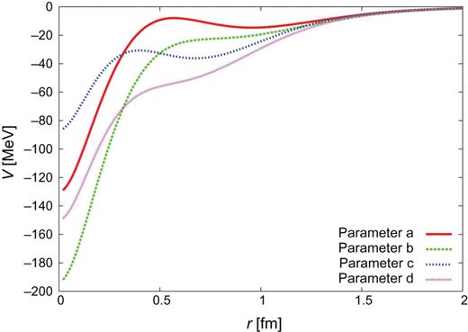
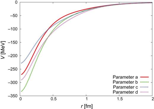
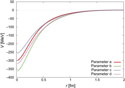
|$Y_{c}N$| CTNN potential for the |$\Lambda _{c}N$| single channel.
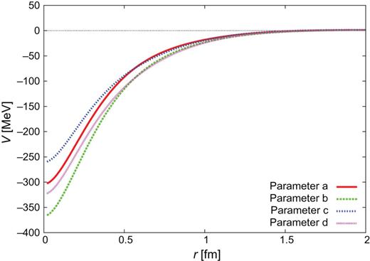
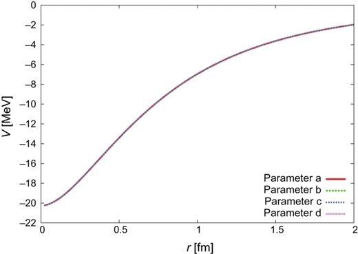
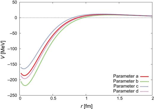
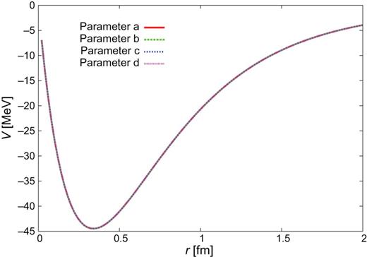
|$Y_{c}N$| CTNN potential for the |$\Sigma _{c}N$| single channel.
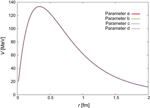
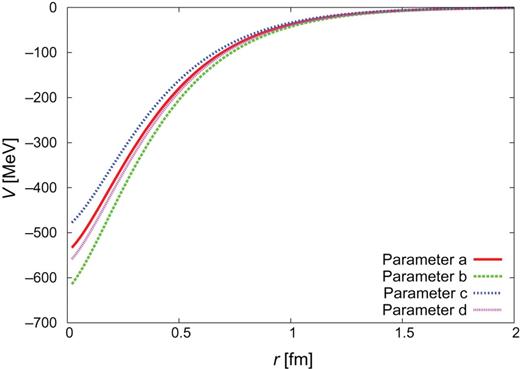
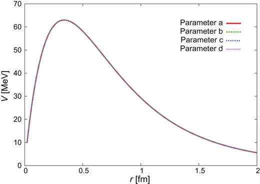
|$Y_{c}N$| CTNN potential for the |$\Sigma _{c}^{*}N$| single channel.
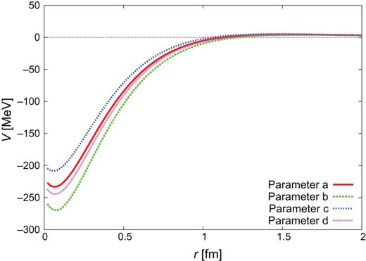
|$Y_{c}N$| CTNN potential for the |$\Lambda _{c}N$|-|$\Sigma _{c}N$| channels.
|$Y_{c}N$| CTNN potential for the |$\Lambda _{c}N$|–|$\Sigma _{c}^{*}N$| channels.
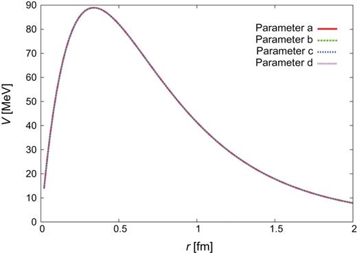
|$Y_{c}N$| CTNN potential for the |$\Sigma _{c}N$|–|$\Sigma _{c}^{*}N$| channels.
3. |$Y_{c}N$| bound states
This method has been applied to various bound state problems and was proved to give an accurate approximation to the eigenstate energies and wave functions.
Binding energies of |$\Lambda _{c}N$| (|$J^{\pi }$| = |$0^{+}$|) for the CTNN potentials. The probabilities of the |$\Sigma _{c}N$| and |$\Sigma _{c}^{*}N$| channels are also shown.
| |$J^{\pi }=0^{+}$| | CTNN-a | CTNN-b | CTNN-c | CTNN-d |
|---|---|---|---|---|
| B.E. [MeV] | — | — | 1.72 |$\times 10^{-3}$| | 1.37 |
| (|$+$|Coulomb) | (0.56) | |||
| Scattering length [fm] | |$-$|3.64 | |$-$|65.15 | 130.93 | 5.31 |
| Probability (|$\Lambda _{c}N$|) [%] | — | — | 99.97 | 99.29 |
| Probability (|$\Sigma _{c}N$|) [%] | — | — | 7.0 |$\times 10^{-3}$| | 0.20 |
| Probability (|$\Sigma _{c}^{*}N$|) [%] | — | — | 2.1 |$\times 10^{-2}$| | 0.51 |
Binding energies of |$\Lambda _{c}N$| (|$J^{\pi }$| = |$1^{+}$|) for the CTNN potentials. The probabilities of the coupled D-wave |$\Lambda _{c}N$| and |$\Sigma _{c}N$| and |$\Sigma _{c}^{*}N$| channels are also shown.
| |$J^{\pi }=1^{+}$| | CTNN-a | CTNN-b | CTNN-c | CTNN-d |
|---|---|---|---|---|
| B.E. [MeV] | — | 2.62 |$\times 10^{-4}$| | 1.97 |$\times 10^{-2}$| | 1.57 |
| (|$+$|Coulomb) | (0.72) | |||
| Scattering length [fm] | |$-$|4.11 | 337.53 | 39.27 | 5.01 |
| Probability (|$\Lambda _{c}N$|) [%] | — | 99.99 | 99.90 | 99.23 |
| Probability (|$\Sigma _{c}N$|) [%] | — | 6.1 |$\times 10^{-3}$| | 5.0 |$\times 10^{-2}$| | 0.39 |
| (D-wave (|$^{3}D_{1}$|)) | — | 5.6 |$\times 10^{-3}$| | 4.6 |$\times 10^{-2}$| | 0.35 |
| Probability (|$\Sigma _{c}^{*}N$|) [%] | — | 5.8 |$\times 10^{-3}$| | 4.7 |$\times 10^{-2}$| | 0.38 |
| (D-wave (|$^{5}D_{1}$|)) | — | 3.9 |$\times 10^{-3}$| | 3.3 |$\times 10^{-2}$| | 0.25 |
The |$Y_{c}N$| binding energies are given in Tables 6 and 7. The |$\Lambda _{c}n$| system (|$J^{\pi }=0^{+}$| or |$1^{+}$|) without the Coulomb potential has a bound state for the |$Y_{c}N$| CTNN parameters b, c, and d. The CTNN-b and c potentials allow very shallow bound states and the CTNN-d potential gives a larger binding energy. The result indicates that there is a strong QCM repulsion at short distances for the CTNN-a and b parameters. On the other hand, the |$\Lambda _{c}p$| system with the Coulomb potential has a bound state only for the parameter CTNN-d.
As a cross check, we also calculate the |$\Lambda _{c}N$| scattering lengths for the CTNN potentials. These results are consistent with the binding energies (see Tables 6 and 7.)
The above results show that the binding energies of the |$J^{\pi }=1^{+}$| states are larger than those of |$J^{\pi }=0^{+}$|. This is consistent with the previous study [11].
Table 7 also shows the probabilities of the coupled channels. For all the parameter sets and the total angular momenta, the probability of |$\Lambda _{c}N$| is more than 99%. In the case of |$J^{\pi }=0^{+}$|, the probabilities of |$\Sigma _{c}^{*}N(^{5}D_{0}$|) are larger than those of |$\Sigma _{c}N(^{1}S_{0}$|). On the other hand, in the case of |$J^{\pi }=1^{+}$|, the respective total probabilities of |$\Sigma _{c}N$| and |$\Sigma _{c}^{*}N$| are almost equal. Looking closely, |$\Sigma _{c}N\ (^{3}S_{1})$| and |$\Sigma _{c}^{*}N\ (^{5}D_{1})$| contribute largely to the results. These observations can be explained with the contributions of the strong tensor force between the |$\Lambda _{c}N$| (|$L=0$|) and |$\Sigma _{c}N/\Sigma _{c}^{*}N$| (|$L=2$|) channels.
4. |$\Lambda _{c} NN$| systems
4.1. Effects of channel couplings
In the previous section, we found that the probabilities of the |$\Lambda _{c}N$| component are almost 100% and the mixings of |$\Sigma _{c}N$| or |$\Sigma _{c}^{*}N$| are small. However, the effects of the |$\Sigma _{c}N$|–|$\Sigma _{c}^{*}N$| channel coupling are important in binding the |$\Lambda _{c}N$| system, because the single-channel calculations of |$\Lambda _{c}N$| do not show any binding solutions for all the CTNN-a–d potentials.
In Table 8, we show the scattering lengths obtained for partially coupled systems, i.e., |$\Lambda _{c}N$|, |$\Lambda _{c}N$|–|$\Sigma _{c}N$|, and |$\Lambda _{c}N$|–|$\Sigma _{c}^{*}N$|. It is found that only the CTNN-d potential allows bound states in the |$\Lambda _{c}N$|–|$\Sigma _{c}^{*}N$| (|$0^{+}$| and |$1^{+}$|) and the |$\Lambda _{c}N$|–|$\Sigma _{c}N$| (|$1^{+}$|) systems. In particular, effect of the |$\Sigma _{c}^{*}N$| (|$0^{+}$|) channel is large because no bound state is found without this channel. This indicates that the tensor force from the one-pion exchange, which induces the coupling between |$\Sigma _{c}^{*}N$||$\Big ({}^{5}D_{0}\Big )$| and |$\Lambda _{c}N$||$\Big ({}^{1}S_{0}\Big )$|, is significant. Similarly, the contributions of the tensor force and |$\Sigma _{c}N$|–|$\Sigma _{c}^{*}N$| couplings are found to be important for the |$J^{\pi }=1^{+}$| state.
4.2. Effective |$\Lambda _{c}N$| potential
Now, we use only the CTNN-d |$Y_{c}N$| potential to construct the effective potential. By reproducing the binding energies and the scattering lengths in Tables 6 and 7, we search for values of the parameters in Eq. (13). In doing so, we assume that the first term [|$V_{1}$| of Eq. (13)] is an attractive potential like the OBE potential and the second term (|$V_{2}$|) is repulsive like the QCM repulsion. Accordingly, |$b_{2}$| is taken to be the radius of the quark wave function, |$b_{2}=0.5$| fm. On the other hand, |$b_{1}=0.9$| fm is chosen to represent a typical range of the meson exchange potential which couples |$\Sigma _{c}N$| and |$\Sigma _{c}^{*}N$| to |$\Lambda _{c}N$|.
Scattering lengths in fm, and two-body binding energies in MeV for the cases that the coupled channels are reduced to |$\Lambda _{c}N$| only, |$\Lambda _{c}N$|–|$\Sigma _{c}N$|, or |$\Lambda _{c}N$|–|$\Sigma _{c}^{*}N$|.
| |$\Lambda
_{c}N$|–|$\Sigma
_{c}N$|–|$\Sigma
_{c}^{*}N$| | |$\Lambda
_{c}N$| | |$\Lambda
_{c}N$|–|$\Sigma
_{c}N$| | |$\Lambda
_{c}N$|–|$\Sigma
_{c}^{*}N$| | |||||
|---|---|---|---|---|---|---|---|---|
| ___________________ | _______________ | _____________ | _____________ | |||||
| |$J^{\pi }$| | |$0^{+}$| | |$1^{+}$| | |$0^{+}$| | |$1^{+}$| | |$0^{+}$| | |$1^{+}$| | |$0^{+}$| | |$1^{+}$| |
| CTNN-a | |$-$|3.63 | |$-$|4.10 | |$-$|1.11 | |$-$|1.11 | |$-$|1.16 | |$-$|2.07 | |$-$|3.13 | |$-$|2.09 |
| CTNN-b | |$-$|63.25 | 398.67 | |$-$|2.62 | |$-$|2.62 | |$-$|2.78 | |$-$|6.74 | |$-$|20.84 | |$-$|7.00 |
| CTNN-c | 139.07 | 39.96 | |$-$|3.01 | |$-$|3.01 | |$-$|3.19 | |$-$|8.61 | |$-$|48.56 | |$-$|9.00 |
| CTNN-d | 5.32 | 5.02 | |$-$|28.59 | |$-$|28.59 | |$-$|44.65 | 9.79 | 6.01 | 9.36 |
| B.E. | 1.37 | 1.56 | — | — | — | 0.36 | 1.04 | 0.39 |
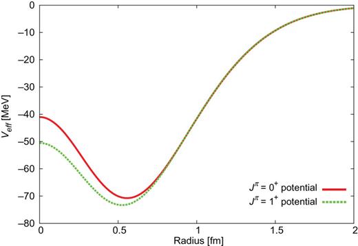
|$\Lambda _{c}N$| effective potentials for |$J^{\pi }=0^{+}$| and |$1^{+}$|.
It is obvious that the spin-dependent potential is weak. This is a consequence of the heavy quark spin symmetry [25–28].
4.3. |$\Lambda _{c}NN$| bound states
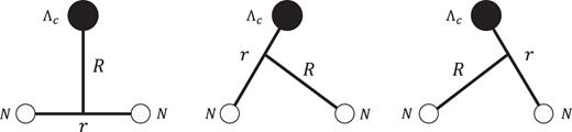
Jacobi coordinates for |$\Lambda _{c}NN$| system.
Next, we study the |$\Lambda _{c}NN$| three-body system by using the above |$\Lambda _{c}N$| effective potential. In the calculation, we adopt the Jacobi coordinates shown in Fig. 10. The angular momenta |$l$| and |$L$| are defined corresponding to |$r$| and |$R$|, respectively. On the other hand, we define the spin for two nucleons as |$S_{NN}$|, and the total spin of the systems as |$S_{tot}$|. For the isoscalar case, the binding energy is calculated from the threshold of |$\Lambda _{c}$| plus the deuteron, while for the case |$I=1$|, the calculation is from the threshold of the bound |$\Lambda _{c}N$| (binding energy = 1.56 MeV) plus a nucleon.
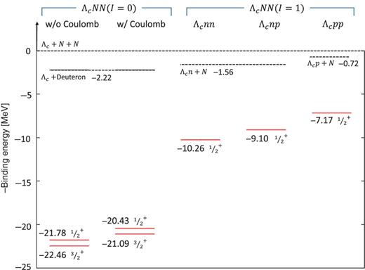
|$\Lambda _{c}NN$| binding energies. The dotted lines are the |$\Lambda _{c}$|–deuteron threshold that is |$2.22$| MeV below the |$\Lambda _{c}NN$| threshold, the threshold of the (|$\Lambda _{c}n$|) |$1^{+}$| bound state plus a nucleon, i.e., |$1.56$| MeV below |$\Lambda _{c}NN$|, and the threshold of the (|$\Lambda _{c}p$|) |$1^{+}$| bound state plus a nucleon, i.e., |$0.72$| MeV below |$\Lambda _{c}NN$|.
We again use GEM [19] to solve the three-body problem. The binding energies of the |$\Lambda _{c}NN$| three-body system with the |$\Lambda _{c}N$| effective potential are shown in Fig. 11. The left two plots show the results for |$I=0$| without and with the Coulomb potential, respectively. The others represent the |$I=1$| results for |$\Lambda _{c}nn$|, |$\Lambda _{c}np$|, and |$\Lambda _{c}pp$|. For each system, we find a bound state. Because the spin–spin interaction between |$\Lambda _{c} $| and |$N$| is weak (Table 7), the binding energies of |$J^{\pi }=\frac {1}{2}^{+}$| and |$\frac {3}{2}^{+}$| are close to each other for the case of |$I=0$|. These results agree well with the heavy quark spin symmetry [25]. In the present calculation, we find that the |$\frac {3}{2}^{+}$| state is lower in energy than the |$\frac {1}{2}^{+}$| state by about |$0.7$| MeV. These results are consistent with a recent three-body calculation [12], which also favors |$\frac {3}{2}^{+}$||$\Lambda _{c}NN$| as the lowest state. The effect of the Coulomb potential between |$\Lambda _{c}$| and proton is smaller than the difference between the |$I=0$| and 1 results.
|$\Lambda _{c}NN$| binding energies and particle distances for the |$I=0$| bound states.
| Binding energy [MeV] | (From threshold) | |$r$| [fm] | |$R$| [fm] | |
|---|---|---|---|---|
| |$\Lambda _{c}np$| w/o Coulomb |$J^{\pi }=\frac {1}{2}^{+}$| | 21.78 | 19.56 | 1.91 | 1.34 |
| |$\Lambda _{c}np$| w/o Coulomb |$J^{\pi }=\frac {3}{2}^{+}$| | 22.46 | 20.24 | 1.90 | 1.32 |
| |$\Lambda _{c}np$| w/ Coulomb |$J^{\pi }=\frac {1}{2}^{+}$| | 20.43 | 18.21 | 1.93 | 1.36 |
| |$\Lambda _{c}np$| w/ Coulomb |$J^{\pi }=\frac {3}{2}^{+}$| | 21.09 | 18.87 | 1.91 | 1.34 |
|$\Lambda _{c}NN$| binding energies and particle distances for the |$I=1$| bound states.
| Binding energy [MeV] | (From threshold) | |$r$| [fm] | |$R$| [fm] | |
|---|---|---|---|---|
| |$\Lambda _{c}nn$||$J^{\pi }=\frac {1}{2}^{+}$| | 10.26 | 8.70 | 2.62 | 1.64 |
| |$\Lambda _{c}np$||$J^{\pi }=\frac {1}{2}^{+}$| | 9.10 | 7.54 | 2.67 | 1.68 |
| |$\Lambda _{c}pp$||$J^{\pi }=\frac {1}{2}^{+}$| | 7.17 | 6.35 | 2.78 | 1.75 |
Tables 9 and 10 show the mean distances in the bound state, where |$r$| is the root mean square (rms) distance between the nucleons, and |$R$| is rms distance between |$\Lambda _{c}$| and the center of |$NN$|. These tables illustrate that the mean |$NN$| separations, |$r$|, are significantly smaller than the mean distance of |$p$|–|$n$| in the deuteron, about 3.8 fm. Namely, the |$\Lambda _{c}$| attraction to the nucleon makes the |$\Lambda _{c}NN$| system shrink. It is also observed that |$R$| is smaller than |$r$|. Thus we can draw an intuitive picture that the nucleons go around |$\Lambda _{c}$| sitting at the center in the |$\Lambda _{c}NN$| system. This property is also seen in the hypernuclear system, but the attractive force in the charmed nuclear system is stronger than that in the hypernuclear system.
We may check whether these results depend on the choice of the |$NN$| potential. Here we have used the Minnesota potential, which is known to have a weak repulsive core. For comparison, we replace the Minnesota potential by the AV8|$^{\prime }$| potential [29] and apply it to the |$I=1$||$\Lambda _{c}nn$| system. For the |$I=0$||$\Lambda _{c}NN$| systems, the comparison is not appropriate because the AV8|$^{\prime }$| contains the tensor force which make the D-wave components couple.
Then we obtain the binding energy BE = 11.93 [MeV] and the rms distances as |$r=2.41$| [fm] and |$R=1.54$| [fm]. These results can be compared to the first line of Table 10. One sees that they are consistent with each other. Thus we conclude that the qualitative behavior of the |$\Lambda _{c}NN$| bound state is independent of the choice of the |$NN$| potential.
5. Conclusion
We have examined the interactions between the ground-state charmed baryons |$\Lambda _c$|, |$\Sigma _c$|, and |$\Sigma _c^*$| and the nucleon |$N$|. Potential models are proposed, which are composed of the long-range one-boson exchange (OBE) force and the short-range quark exchange force based on the quark cluster model (QCM). We also include the Coulomb potential between the charged baryons. The parameters in the model, the cutoffs and the coupling constant of the |$\sigma $| meson, are determined so that the |$NN$| data are reproduced in the same model. By fitting the deuteron binding energy and the S-wave scattering lengths, four parameter sets are obtained.
We have applied these potentials to the two-body |$\Lambda _cN$|–|$\Sigma _cN$|–|$\Sigma _c^{*}N$| coupled system. The coupled-channel Schrödinger equation is solved to a good precision by the Gaussian expansion method. We find shallow bound |$\Lambda _cN$| states both in |$J^{\pi }=0^+$| and |$1^+$| in two of the four parameter sets. Those parameters are the cases where the ranges of the QCM repulsion are small and thus the quark exchange effect is weaker than the other two. The difference between the |$J^{\pi }=0^+$| [|$\Lambda _c N(^1S_0)$|] and |$1^+$| [|$\Lambda _c N(^3S_1)$|] systems is small, which is a consequence of the heavy quark spin symmetry.
It is not surprising to have a bound state in these channels, because the |$Y_c N$| interactions are similar to those of |$YN$| except for the |$K$| exchange part, while the kinetic energy is suppressed by the heavier mass. Furthermore, the effect of the channel coupling to |$\Sigma _c^* N$| is significant due to the strong tensor force coming from the one-pion exchange. We then conclude that shallow |$\Lambda _c N$| bound states may exist.
Encouraged by the possible existence of the two-body bound states, we further consider three-body |$\Lambda _c NN$| bound states. This is the lightest “charmed nucleus,” which corresponds to the hyper-triton (|$\Lambda pn$|) bound state in the strangeness sector. In order to simplify the calculation, we first construct an effective one-channel (|$\Lambda _c N$|) potential from the fully coupled (|$\Lambda _c N$|–|$\Sigma _c N$|–|$\Sigma ^*_c N$|) calculation. Using the effective one-channel potential, we have solved the three-body Schrödinger equation with the GEM and have obtained bound states with binding energy about 20–22 MeV for |$I=0$| and 7–10 MeV for |$I=1$| from the |$\Lambda _{c} NN$| threshold. The corresponding wave functions indicate that the |$\Lambda _c$| baryon makes the size of the |$NN$| system significantly smaller owing to attractive force. In order to confirm these results, further studies with the full and explicit couplings with the |$\Sigma _cN$| and |$\Sigma ^*_cN$| channels will be necessary.
Acknowledgments
S. M. is supported by the RIKEN Junior Research Associate Program. This work is supported in part by JSPS KAKENHI Grant Nos. 25247036 and 24250294. Y. R. L. was supported by the “Program for Promoting the Enhancement of Research Universities” at Tokyo Institute of Technology in 2014 and partly by NNSFC (No. 11275115). This work is also supported by the Research Abroad and Invitational Program for the Promotion of International Joint Research, Category (C) and the International Physics Leadership Program at Tokyo Tech.
Appendix A. Spin matrix elements of |$Y_{c}N$| OBE potential
|${\boldsymbol L}\cdot \boldsymbol {\mathcal {O}}_1$| is not included in the potential for this calculation.
A.1. |$I=\frac 12$|, |$J^{\pi }=0^+$| coupled system
Tables A1–A3 give the matrix elements of |$\boldsymbol {\mathcal {O}}_{\rm spin}$|, |$\boldsymbol {\mathcal {O}}_{\rm ten}$|, and |$\boldsymbol {\mathcal {O}}_{\rm LS}$| for the channels in |$I=1/2$|, |$J^{\pi }=0^{+}$|. We label the relevant channels by |$i$| and |$j$|, and tabulate the |$ij$| component of the matrix elements |$\left \langle \boldsymbol {\mathcal {O}}\right \rangle _{ij}$|.
The matrix elements of the spin–spin operators |$\left \langle \boldsymbol {\mathcal {O}}_{\rm spin} \right \rangle _{ij}$| for the |$I=\frac 12$|, |$J^{\pi }=0^+$| coupled system.
| |${\rm{i \backslash j}}$| | |$\Lambda _cN(^1S_0)$| | |$\Sigma _cN(^1S_0)$| | |$\Sigma _c^*N(^5D_0)$| |
|---|---|---|---|
| |$\Lambda _cN(^1S_0)$| | |$-3$| | |$-3$| | 0 |
| |$\Sigma _cN(^1S_0)$| | |$-3$| | |$-3$| | 0 |
| |$\Sigma _c^*N(^5D_0)$| | 0 | 0 | 1 |
| |${\rm{i \backslash j}}$| | |$\Lambda _cN(^1S_0)$| | |$\Sigma _cN(^1S_0)$| | |$\Sigma _c^*N(^5D_0)$| |
|---|---|---|---|
| |$\Lambda _cN(^1S_0)$| | |$-3$| | |$-3$| | 0 |
| |$\Sigma _cN(^1S_0)$| | |$-3$| | |$-3$| | 0 |
| |$\Sigma _c^*N(^5D_0)$| | 0 | 0 | 1 |
The matrix elements of the tensor operators |$\left \langle \boldsymbol {\mathcal {O}}_{\rm ten} \right \rangle _{ij}$| for the |$I=\frac 12$|, |$J^{\pi }=0^+$| coupled system.
| |${\rm{i \backslash j}}$| | |$\Lambda _cN(^1S_0)$| | |$\Sigma _cN(^1S_0)$| | |$\Sigma _c^*N(^5D_0)$| |
|---|---|---|---|
| |$\Lambda _cN(^1S_0)$| | 0 | 0 | |$-\sqrt 6$| |
| |$\Sigma _cN(^1S_0)$| | 0 | 0 | |$-\sqrt 6$| |
| |$\Sigma _c^*N(^5D_0)$| | |$-\sqrt 6$| | |$-\sqrt 6$| | |$-2$| |
| |${\rm{i \backslash j}}$| | |$\Lambda _cN(^1S_0)$| | |$\Sigma _cN(^1S_0)$| | |$\Sigma _c^*N(^5D_0)$| |
|---|---|---|---|
| |$\Lambda _cN(^1S_0)$| | 0 | 0 | |$-\sqrt 6$| |
| |$\Sigma _cN(^1S_0)$| | 0 | 0 | |$-\sqrt 6$| |
| |$\Sigma _c^*N(^5D_0)$| | |$-\sqrt 6$| | |$-\sqrt 6$| | |$-2$| |
The matrix elements of the orbital–spin operators |$\left \langle \boldsymbol {\mathcal {O}}_{\rm LS} \right \rangle _{ij}$| for the |$I=\frac 12$|, |$J^{\pi }=0^+$| coupled system.
| |${\rm{i \backslash j}}$| | |$\Lambda _cN(^1S_0)$| | |$\Sigma _cN(^1S_0)$| | |$\Sigma _c^*N(^5D_0)$| |
|---|---|---|---|
| |$\Lambda _cN(^1S_0)$| | 0 | 0 | 0 |
| |$\Sigma _cN(^1S_0)$| | 0 | 0 | 0 |
| |$\Sigma _c^*N(^5D_0)$| | 0 | 0 | |$-3$| |
| |${\rm{i \backslash j}}$| | |$\Lambda _cN(^1S_0)$| | |$\Sigma _cN(^1S_0)$| | |$\Sigma _c^*N(^5D_0)$| |
|---|---|---|---|
| |$\Lambda _cN(^1S_0)$| | 0 | 0 | 0 |
| |$\Sigma _cN(^1S_0)$| | 0 | 0 | 0 |
| |$\Sigma _c^*N(^5D_0)$| | 0 | 0 | |$-3$| |
A.2. |$I=\frac 12$|, |$J^{\pi }=1^+$| coupled system
For |$I=1/2$|, |$J^{\pi }=1^{+}$|, the matrix elements are given in Tables A4–A6.
The matrix elements of the spin–spin operators |$\left \langle \boldsymbol {\mathcal {O}}_{\rm spin} \right \rangle _{ij}$| for the |$I=\frac 12$|, |$J^{\pi }=1^+$| coupled system.
| |${\rm{i \backslash j}}$| | |$\Lambda _cN(^3S_1)$| | |$\Sigma _cN(^3S_1)$| | |$\Sigma _c^*N(^3S_1)$| | |$\Lambda _cN(^3D_1)$| | |$\Sigma _cN(^3D_1)$| | |$\Sigma _c^*N(^3D_1)$| | |$\Sigma _c^*N(^5D_1)$| |
|---|---|---|---|---|---|---|---|
| |$\Lambda _cN(^3S_1)$| | 1 | 1 | |$- \sqrt {{8 \over 3}}$| | 0 | 0 | 0 | 0 |
| |$\Sigma _cN(^3S_1)$| | 1 | 1 | |$- \sqrt {{8 \over 3}}$| | 0 | 0 | 0 | 0 |
| |$\Sigma _c^*N(^3S_1)$| | |$- \sqrt {{8 \over 3}}$| | |$- \sqrt {{8 \over 3}}$| | |$-\frac 53$| | 0 | 0 | 0 | 0 |
| |$\Lambda _c N(^3D_1)$| | 0 | 0 | 0 | 1 | 1 | |$- \sqrt {{8 \over 3}}$| | 0 |
| |$\Sigma _cN(^3D_1)$| | 0 | 0 | 0 | 1 | 1 | |$- \sqrt {{8 \over 3}}$| | 0 |
| |$\Sigma _c^*N(^3D_1)$| | 0 | 0 | 0 | |$- \sqrt {{8 \over 3}}$| | |$- \sqrt {{8 \over 3}}$| | |$-\frac 53$| | 0 |
| |$\Sigma _c^*N(^5D_1)$| | 0 | 0 | 0 | 0 | 0 | 0 | 1 |
The matrix elements of the tensor operators |$\left \langle \boldsymbol {\mathcal {O}}_{\rm ten} \right \rangle _{ij}$| for the |$I=\frac 12$|, |$J^{\pi }=1^+$| coupled system.
| |${\rm{i \backslash j}}$| | |$\Lambda _cN(^3S_1)$| | |$\Sigma _cN(^3S_1)$| | |$\Sigma _c^*N(^3S_1)$| | |$\Lambda _cN(^3D_1)$| | |$\Sigma _cN(^3D_1)$| | |$\Sigma _c^*N(^3D_1)$| | |$\Sigma _c^*N(^5D_1)$| |
|---|---|---|---|---|---|---|---|
| |$\Lambda _cN(^3S_1)$| | 0 | 0 | 0 | |$\sqrt 8$| | |$\sqrt 8$| | |$\frac {1}{\sqrt 3}$| | |$\sqrt 3$| |
| |$\Sigma _cN(^3S_1)$| | 0 | 0 | 0 | |$\sqrt 8$| | |$\sqrt 8$| | |$\frac {1}{\sqrt 3}$| | |$\sqrt 3$| |
| |$\Sigma _c^*N(^3S_1)$| | 0 | 0 | 0 | |$\frac {1}{\sqrt 3}$| | |$\frac {1}{\sqrt 3}$| | |$ - {{\sqrt 2 } \over 3}$| | |$-\sqrt 2$| |
| |$\Lambda _c N(^3D_1)$| | |$\sqrt 8$| | |$\sqrt 8$| | |$\frac {1}{\sqrt 3}$| | |$-2$| | |$-2$| | |$-\frac {1}{\sqrt 6}$| | |$\sqrt {{3 \over 2}} $| |
| |$\Sigma _cN(^3D_1)$| | |$\sqrt 8$| | |$\sqrt 8$| | |$\frac {1}{\sqrt 3}$| | |$-2$| | |$-2$| | |$-\frac {1}{\sqrt 6}$| | |$\sqrt {{3 \over 2}} $| |
| |$\Sigma _c^*N(^3D_1)$| | |$\frac {1}{\sqrt 3}$| | |$\frac {1}{\sqrt 3}$| | |$ - {{\sqrt 2 } \over 3}$| | |$-\frac {1}{\sqrt 6}$| | |$-\frac {1}{\sqrt 6}$| | |$\frac 13$| | |$-1$| |
| |$\Sigma _c^*N(^5D_1)$| | |$\sqrt 3$| | |$\sqrt 3$| | |$-\sqrt 2$| | |$\sqrt {{3 \over 2}} $| | |$\sqrt {{3 \over 2}} $| | |$-1$| | |$-1$| |
The matrix elements of the orbital–spin operators |$\left \langle \boldsymbol {\mathcal {O}}_{\rm LS} \right \rangle _{ij}$| for the |$I=\frac 12$|, |$J^{\pi }=1^+$| coupled system.
| |${\rm{i \backslash j}}$| | |$\Lambda _cN(^3S_1)$| | |$\Sigma _cN(^3S_1)$| | |$\Sigma _c^*N(^3S_1)$| | |$\Lambda _cN(^3D_1)$| | |$\Sigma _cN(^3D_1)$| | |$\Sigma _c^*N(^3D_1)$| | |$\Sigma _c^*N(^5D_1)$| |
|---|---|---|---|---|---|---|---|
| |$\Lambda _cN(^3S_1)$| | 0 | 0 | 0 | 0 | 0 | 0 | 0 |
| |$\Sigma _cN(^3S_1)$| | 0 | 0 | 0 | 0 | 0 | 0 | 0 |
| |$\Sigma _c^*N(^3S_1)$| | 0 | 0 | 0 | 0 | 0 | 0 | 0 |
| |$\Lambda _c N(^3D_1)$| | 0 | 0 | 0 | |$-3$| | |$-3$| | 0 | 0 |
| |$\Sigma _cN(^3D_1)$| | 0 | 0 | 0 | |$-3$| | |$-3$| | 0 | 0 |
| |$\Sigma _c^*N(^3D_1)$| | 0 | 0 | 0 | 0 | 0 | |$\frac 32$| | |$-\frac 32$| |
| |$\Sigma _c^*N(^5D_1)$| | 0 | 0 | 0 | 0 | 0 | |$-\frac 32$| | |$-\frac 52$| |
Appendix B. Definitions of the radial functions and coupling constants
B.1. The explicit forms of the radial functions
where |$m$| is the mass of the exchanged meson and |$q$| is the four-dimensional momentum of the meson. We use the following values of the meson masses: |$m_{\pi }=137.27$| [MeV], |$m_{\sigma }=600.0$| [MeV].
B.2. The coupling constants for the meson exchange potentials
|$C_{\pi }$| for the |$Y_{c}N$| systems.
| |$C_{\pi }$| | |$\Lambda _cN$| | |$\Sigma _cN$| | |$\Sigma _c^*N$| |
|---|---|---|---|
| |$\Lambda _cN$| | 0 | |$\left( { - {{\sqrt 6 } \over 2}{g_2}{g_A}} \right)$| | |$ - \left( {{{\sqrt 6 } \over 2}{g_4}{g_A}} \right)$| |
| |$\Sigma _cN$| | |$\left (-g_{1}g_{A}\right )$| | |$\left (-g_{3}g_{A}\right )$| | |
| |$\Sigma _c^*N$| | |$(g_{5}g_{A})$| |
|$C_{\sigma }$| for the |$Y_{c}N$| systems.
| |$C_{\sigma }$| | |$\Lambda _cN$| | |$\Sigma _cN$| | |$\Sigma _c^*N$| |
|---|---|---|---|
| |$\Lambda _cN$| | |$(2l_{B}h_{\sigma })$| | ||
| |$\Sigma _cN$| | |$(-l_{S}h_{\sigma })$| | ||
| |$\Sigma _c^*N$| | |$(-l_{S}h_{\sigma })$| |
| |$C_{\sigma }$| | |$\Lambda _cN$| | |$\Sigma _cN$| | |$\Sigma _c^*N$| |
|---|---|---|---|
| |$\Lambda _cN$| | |$(2l_{B}h_{\sigma })$| | ||
| |$\Sigma _cN$| | |$(-l_{S}h_{\sigma })$| | ||
| |$\Sigma _c^*N$| | |$(-l_{S}h_{\sigma })$| |
|$Y_{c}N$| potential |$C_{\pi }$| values.
| |$C_{\pi }$| | |$\Lambda _cN$| | |$\Sigma _cN$| | |$\Sigma _c^*N$| |
|---|---|---|---|
| |$\Lambda _cN$| | 0 | |$\phantom {-}0.92$| | |$-1.53$| |
| |$\Sigma _cN$| | |$-1.18$| | |$-1.02$| | |
| |$\Sigma _c^*N$| | |$-1.77$| |
| |$C_{\pi }$| | |$\Lambda _cN$| | |$\Sigma _cN$| | |$\Sigma _c^*N$| |
|---|---|---|---|
| |$\Lambda _cN$| | 0 | |$\phantom {-}0.92$| | |$-1.53$| |
| |$\Sigma _cN$| | |$-1.18$| | |$-1.02$| | |
| |$\Sigma _c^*N$| | |$-1.77$| |
|$Y_{c}N$| potential |$C_{\sigma }$| values.
| |$C_{\sigma }$| | |$\Lambda _cN$| | |$\Sigma _cN$| | |$\Sigma _c^*N$| |
|---|---|---|---|
| |$\Lambda _cN$| | |$(-6.2h_{\sigma })$| | ||
| |$\Sigma _cN$| | |$(-6.2h_{\sigma })$| | ||
| |$\Sigma _c^*N$| | |$(-6.2h_{\sigma })$| |
| |$C_{\sigma }$| | |$\Lambda _cN$| | |$\Sigma _cN$| | |$\Sigma _c^*N$| |
|---|---|---|---|
| |$\Lambda _cN$| | |$(-6.2h_{\sigma })$| | ||
| |$\Sigma _cN$| | |$(-6.2h_{\sigma })$| | ||
| |$\Sigma _c^*N$| | |$(-6.2h_{\sigma })$| |
|$C_{\pi }$| for the |$NN$| systems.
| |$C_{\pi }$| | |$NN(I=0)$| | |$NN(I=1)$| |
|---|---|---|
| |$NN(I=0)$| | |$\frac {1}{2}g_{A}^2$| | |
| |$NN(I=1)$| | |$\frac {3}{2}g_{A}^2$| |
| |$C_{\pi }$| | |$NN(I=0)$| | |$NN(I=1)$| |
|---|---|---|
| |$NN(I=0)$| | |$\frac {1}{2}g_{A}^2$| | |
| |$NN(I=1)$| | |$\frac {3}{2}g_{A}^2$| |
|$C_{\sigma }$| for the |$NN$| systems.
| |$C_{\sigma }$| | |$NN(I=0)$| | |$NN(I=1)$| |
|---|---|---|
| |$NN(I=0)$| | |$-h_{\sigma }^{2}$| | |
| |$NN(I=1)$| | |$-h_{\sigma }^{2}$| |
| |$C_{\sigma }$| | |$NN(I=0)$| | |$NN(I=1)$| |
|---|---|---|
| |$NN(I=0)$| | |$-h_{\sigma }^{2}$| | |
| |$NN(I=1)$| | |$-h_{\sigma }^{2}$| |
Appendix C. |$Y_{c}N$| potentials
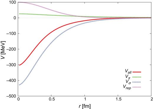
|$Y_{c}N$| CTNN potential for |$\Lambda _{c}N$| single channel.
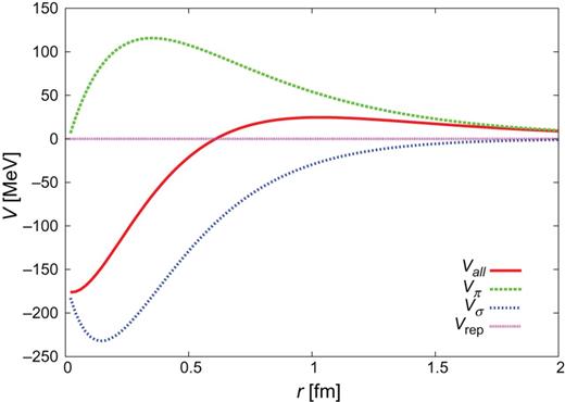
|$Y_{c}N$| CTNN potential for |$\Sigma _{c}N$| single channel.
|$Y_{c}N$| CTNN potential for |$\Sigma _{c}^{*}N$| single channel.
|$\Sigma _{c}N(^{3}S_{1})$| diagonal potential.
|$\Sigma _{c}^{*}N(^{3}S_{1})$| diagonal potential.
|$\Lambda _{c}N(^{3}D_{1})$| diagonal potential.
|$\Sigma _{c}N(^{3}D_{1})$| diagonal potential.
Here we show the shapes of the |$Y_{c}N$| potentials in the present study. The potentials for |$J^{\pi }=0^{+}$| are given in Figs. C1–C3 in Sect. 2.4.
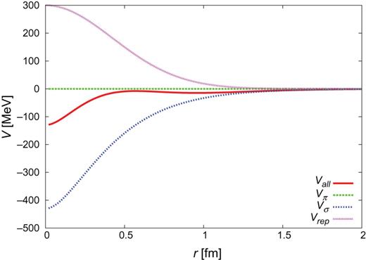
C.1. Components of the |$Y_{c}N$| CTNN-a potential (|$J^{\pi }=0^{+}$|)
The individual contributions of one-pion exchange, one-|$\sigma $| exchange, and QCM repulsion are given in Figs. C1–C3 for the |$J^{\pi }=0^{+}$| CTNN-a potential. One sees that one-|$\sigma $| exchange is strongly attractive, so that even with the QCM repulsion the total potential becomes attractive. Similar behavior is also observed for the CTNN-b, -c, and -d potentials.
C.2. |$Y_{c}N$| potentials(|$J^{\pi }=1^{+}$|)
|$\Sigma _{c}^{*}N(^{3}D_{1})$| diagonal potential.
|$\Sigma _{c}^{*}N(^{5}D_{1})$| diagonal potential.
|$\Lambda _{c}N(^{3}S_{1})$|–|$\Sigma _{c}N(^{3}S_{1})$|.
Figures C4–C29 show the |$J^{\pi }=1^{+}\ Y_{c}N$| potentials. The four lines correspond to the four choices of the parameter sets, a–d. The potential for the diagonal |$\Lambda _{c}N(^{3}S_{1})$| channel is not shown here as it coincides with that for |$\Lambda _{c}N(^{1}S_{0})$|. The off-diagonal potential |$\Lambda _{c}N(^{3}S_{1}- {}^{3}D_{1}$|) is zero.
|$\Lambda _{c}N(^{3}S_{1})$|–|$\Sigma _{c}^{*}N(^{3}S_{1})$|.
|$\Lambda _{c}N(^{3}S_{1})$|–|$\Sigma _{c}N(^{3}D_{1})$|.
|$\Lambda _{c}N(^{3}S_{1})$|–|$\Sigma _{c}^{*}N(^{3}D_{1})$|.
|$\Lambda _{c}N(^{3}S_{1})$|–|$\Sigma _{c}^{*}N(^{3}D_{1})$|.
|$\Sigma _{c}N(^{3}S_{1})$|–|$\Sigma _{c}^{*}N(^{3}S_{1})$|.
|$\Sigma _{c}N(^{3}S_{1})$|–|$\Lambda _{c}N(^{3}D_{1})$|.
|$\Sigma _{c}N(^{3}S_{1})$|–|$\Sigma _{c}N(^{3}D_{1})$|.
|$\Sigma _{c}N(^{3}S_{1})$|–|$\Sigma _{c}^{*}N(^{3}D_{1})$|.
|$\Sigma _{c}N(^{3}S_{1})$|–|$\Sigma _{c}^{*}N(^{5}D_{1})$|.
|$\Sigma {c}^{*}N(^{3}S_{1})$|–|$\Lambda _{c}N(^{3}D_{1})$|.
|$\Sigma {c}^{*}N(^{3}S_{1})$|–|$\Sigma _{c}N(^{3}D_{1})$|.
|$\Sigma {c}^{*}N(^{3}S_{1})$|–|$\Sigma _{c}^{*}N(^{3}D_{1})$|.

|$\Sigma {c}^{*}N(^{3}S_{1})$|–|$\Sigma _{c}^{*}N(^{5}D_{1})$|.
|$\Lambda {c}N(^{3}D_{1})$|–|$\Sigma _{c}N(^{3}D_{1})$|.
|$\Lambda {c}N(^{3}D_{1})$|–|$\Sigma _{c}^{*}N(^{3}D_{1})$|.
|$\Lambda {c}N(^{3}D_{1})$|–|$\Sigma _{c}^{*}N(^{5}D_{1})$|.
|$\Sigma {c}N(^{3}D_{1})$|–|$\Sigma _{c}^{*}N(^{3}D_{1})$|.
|$\Sigma {c}N(^{3}D_{1})$|–|$\Sigma _{c}^{*}N(^{5}D_{1})$|.
|$\Sigma {c}^{*}N(^{3}D_{1})$|–|$\Sigma _{c}^{*}N(^{5}D_{1})$|.
