


Abstract
Focusing on the remnant black holes after merging binary black holes, we show that ringdown gravitational waves of Population III binary black hole mergers can be detected at the rate of for various parameters and functions. This rate is estimated for events with for second-generation gravitational wave detectors such as KAGRA. Here, and are the peak value of the Population III star formation rate and the fraction of binaries, respectively. When we consider only events with , the event rate becomes . This suggest that for a remnant black hole spin of we have an event rate of quasinormal modes with of less than , while it is for third-generation detectors such as the Einstein Telescope. If we detect many Population III binary black hole mergers, it may be possible to constrain the Population III binary evolution paths not only by the mass distribution but also by the spin distribution.
1. Introduction
In our previous paper [4], using the recent population synthesis results of Population III (Pop III) massive BBHs [5,6], we discussed the event rate of QNM GWs by second-generation gravitational wave detectors such as Advanced LIGO [7], Advanced Virgo [8], and KAGRA [9,10]. Since there are various parameters and functions in the population synthesis calculation, we extensively examine BBH binary formations in this paper. Then, we calculate the remnant BH's mass and the non-dimensional spin via fitting formulas [11], and the event rate for each model.
This paper is organized as follows. In Sect. 2, we summarize our Pop III binary population synthesis calculation, and prepare ten models. In Sect. 3, we show the mass ratio distributions of BBH remnants for each model. The dependences on initial distribution functions, binary parameters, etc. are also discussed. In Sect. 4, we obtain the spin distributions of BBH remnants for various parameters. Using the results presented in the above sections, we calculate the mass and spin distributions of the remnant BHs after merger in Sect. 5, and show the event rates of QNMs for each model in KAGRA. Section 6 is devoted to discussions.
2. Population III binary population synthesis calculation
To estimate the detection rate of GWs from Pop III BBH mergers, it is necessary to know how many Pop III binaries become BBHs which merge within the Hubble time. Here, we use the binary population synthesis method
of Monte Carlo simulation of binary evolutions. The Pop III binary population synthesis code [4–6] has been upgraded from the binary population synthesis code [12]1 for Pop III binaries. In this paper, we calculate the same models as Ref. [6] using the same methods as Ref. [6] in order to obtain the mass ratio distribution and the spin distribution. In this section, we review the calculation method and models. Note that in this paper, we do not consider the kick models and the worst model discussed in Ref. [6] for simplicity, because in these models, BBHs have misaligned spins and the final spins after merger are too complex.
First, we need to give the initial conditions when a binary is born. The initial conditions such as primary mass , mass ratio (where is the secondary mass), separation , and orbital eccentricity are decided by the Monte Carlo method with initial distribution functions such as the initial mass function (IMF), the initial mass ratio function (IMRF), the initial separation function (ISF), and the initial eccentricity function (IEF). For example, in our standard model, we use a flat IMF, a flat IMRF, a logflat ISF, and an IEF with a function . There are no observations of Pop III binaries because they were born at the early universe. Thus, we do not know the initial distribution functions of Pop III binaries from observations. For the IMF, however, the recent simulations [13,14] may suggest a flat IMF, and therefore we adapt the flat IMF. For the other initial distribution functions, we adapt those of the Pop I case, where a Pop I star is a solar-like star. The above set of initial distribution functions is called our standard model of 140 cases with the optimistic core-merger criterion in this paper.
Second, we calculate the evolution of each star, and if the star satisfies a condition of binary interactions, we evaluate the effects of binary interactions and change , , , and . As the binary interactions, we treat the Roche lobe overflow (RLOF), the common envelope (CE) phase, the tidal effect, the supernova effect, and the gravitational radiation. The RLOF is stable mass transfer, while unstable mass transfer becomes the CE phase when the donor star is a giant. Here, we need some parameters for the calculation of the RLOF and CE phases.
Finally, if a binary becomes a BBH, we calculate the merger time from the gravitational radiation reaction, and check whether the BBH can merge within the Hubble time or not. We repeat these calculations and take the statistics of BBH mergers.
To study the dependence of Pop III BBH properties on the initial distribution functions and binary parameters, we calculate ten models with the Pop III binary population synthesis method [5,6] in this paper. Table 1 shows the initial distribution functions and the binary parameters of each model. The columns show the model name, IMF, IEF, the CE parameter , and the loss fraction of transfered stellar matter at the RLOF in each model.
The model parameters in this paper. Each column represents the model name, the initial mass function (IMF), the initial eccentricity function (IEF), the common envelope (CE) parameter , and the loss fraction of the transfer of stellar matter at the Roche lobe overflow (RLOF) in each model.
| Model | IMF | IEF | ||
|---|---|---|---|---|
| our standard | flat | 1 | function | |
| IMF: logflat | 1 | function | ||
| IMF: Salpeter | Salpeter | 1 | function | |
| IEF: const. | flat | const. | 1 | function |
| IEF: | flat | 1 | function | |
| flat | 0.01 | function | ||
| flat | 0.1 | function | ||
| flat | 10 | function | ||
| flat | 1 | 0.5 | ||
| flat | 1 | 1 |
3. The mass ratio distributions of binary black hole remnants
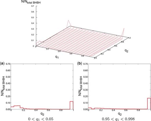
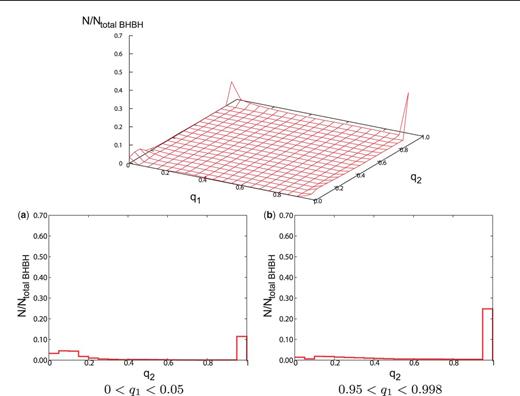
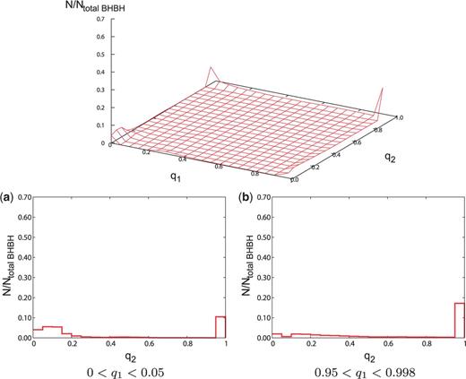
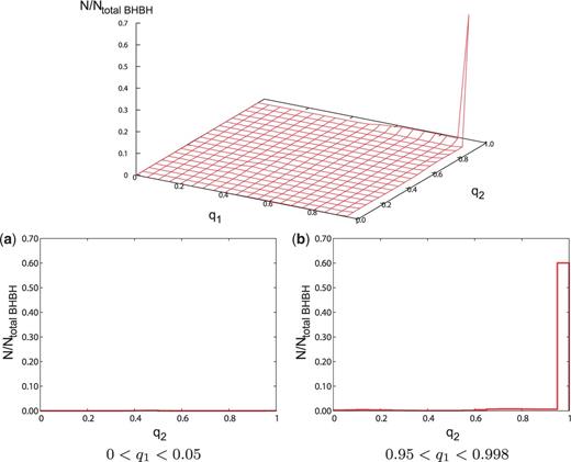
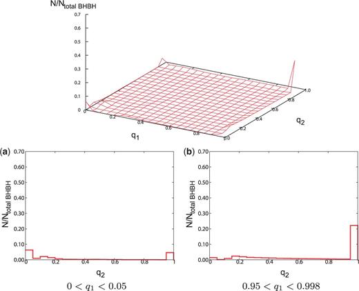
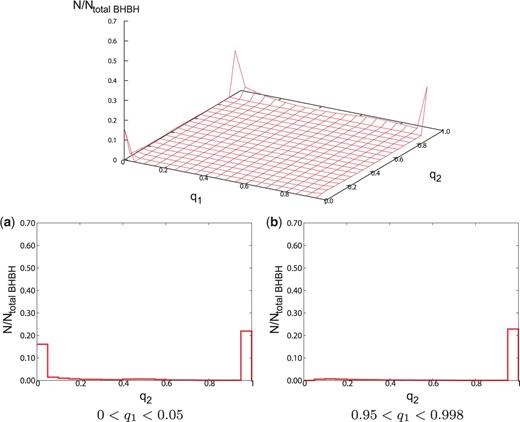
Figures 1–5 show the initial mass ratio distributions and the mass ratio distributions of merging BBHs. The RLOF tends to make binaries of equal mass. Thus, the BBH mass ratio distributions depend on how many binaries evolve via the RLOF. Population III stars with mass evolve as blue giants [5,17]. Thus, in the case of the IMF that light stars are in the majority, the binaries tend to evolve only via the RLOF, not via the CE phase. Therefore, the steeper IMFs tend to derive many equal-mass BBHs. In this calculation, since we adopt the minimum mass ratio as , the initial mass ratio distribution of models with the IMF that light stars are the majority is up to ab initio (see Figs. 1 and 2).
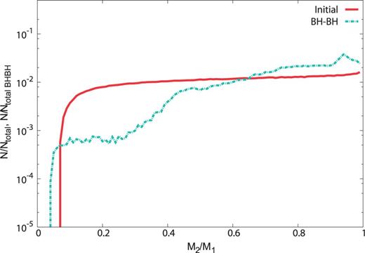
The distribution of mass ratio for our standard model. The distributions of the initial mass ratio and the one when the binaries become BBHs which merge within the Hubble time are shown as red and light blue lines, respectively. The initial mass ratio distribution is normalized by the total binary number , while the one when the binaries become merging BBHs is normalized by the total merging binary number .
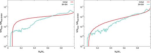
The distributions of mass ratio for the IMF: logflat model (left) and IMF: Salpeter model (right). The format is the same as Fig. 1.
The distributions of mass ratio for the IEF: (left) and IEF: models (right). The format is the same as Fig. 1.

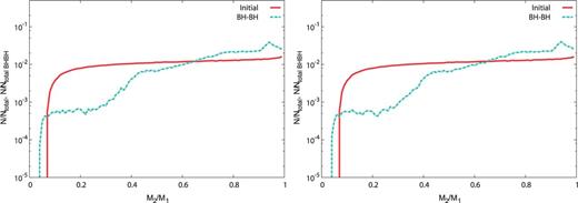
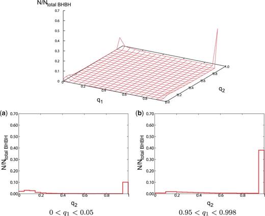
The distributions of mass ratio for the (top left), (top right), and (bottom) models. The format is the same as Fig. 1.
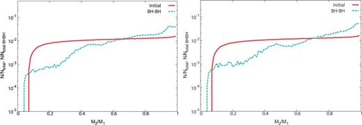
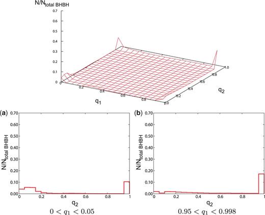
The distributions of mass ratio for the (left) and models (right). The format is the same as Fig. 1.
On the other hand, if we change the IEF, the mass ratio distribution does not change much. Thus, the dependence on the IEF is not so large (see Figs. 1 and 3).
For the CE parameter dependence (see Figs. 1 and 4), small mass ratio binaries in the model of are much fewer than those in the other models. In the model, all the binaries which evolve via the CE phase merge during the CE phase due to too-small . Thus, the merging BBHs in this model evolve only via the RLOF, and become of equal mass by the RLOF. The change is not large between the models with CE parameters and 10.
As for the mass loss fraction (see Figs. 1 and 5), when becomes large, there are three effects. First, binaries tend not to enter the CE phase. Second, the mass accretion by RLOF becomes not to be effective. Third, RLOF tends to finish early. The first effect makes binaries evolve via RLOF. However, the second and third effects have a negative impact on the tendency to become equal mass. Thus, the mass ratio distributions of the and 1 models look similar to our standard model.
4. The spin distributions of binary black hole remnants
We calculate the spin evolution of binaries using the tidal friction. We use the initial spin distribution and the tidal friction calculations as in Refs. [5,12]. When the Pop III star becomes a BH, we calculate the BH's spin using the total angular momentum of the progenitor. If the estimated spin of the BH is more than the Thorne limit [18], we assign the non-dimensional spin parameter .
Figures 6–15 show the spin distributions of merging BBHs and cross-section views of these spin distributions. The spins of merging Pop III BBH can be roughly classified into three types: group 1, in which both BHs have high spins ; group 2, in which both BHs have low spins; and group 3, in which one of the pair has high spin and the other has low spin.
(Top) The distribution of spin parameters for our standard model when each star becomes a BH. and are the spin parameters of the primary and the secondary BHs, respectively. The distribution when the binaries become merging BBHs is normalized by the total merging BBH number , with the grid separation being . (Bottom) Cross-section views of the distribution of spin parameters for our standard model. (a) The distribution of for . We can see that the distribution has bimodal peaks at and . (b) The distribution of for . We see that the large value of is the majority, so that there is a group in which both and are large.
(Top) The distribution of spin parameters for the IMF: logflat model, with . (Bottom) Cross-section views of the distribution of spin parameters for the IMF: logflat model. The format is the same as Fig. 6.
(Top) The distribution of spin parameters for the IMF: Salpeter model, with . (Bottom) Cross-section views of the distribution of spin parameters for the IMF: Salpeter model. The format is the same as Fig. 6.
(Top) The distribution of spin parameters for the IEF: model, with . (Bottom) Cross-section views of the distribution of spin parameters for the IEF: model. The format is the same as Fig. 6.
(Top) The distribution of spin parameters for the IEF: model, with . (Bottom) Cross-section views of the distribution of spin parameters for the IEF: model. The format is the same as Fig. 6.
(Top) The distribution of spin parameters for the model, with . (Bottom) Cross-section views of the distribution of spin parameters for the model. The format is the same as Fig. 6.

(Top) The distribution of spin parameters for the model, with . (Bottom) Cross-section views of the distribution of spin parameters for the model. The format is the same as Fig. 6.
(Top) The distribution of spin parameters for the model, with . (Bottom) Cross-section views of the distribution of spin parameters for the model. The format is the same as Fig. 6.

(Top) The distribution of spin parameters for the model, with . (Bottom) Cross-section views of the distribution of spin parameters for the model. The format is the same as Fig. 6.
(Top) The distribution of spin parameters for the model, with . (Bottom) Cross-section views of the distribution of spin parameters for the model. The format is the same as Fig, 6.
When the BH progenitor evolves via the CE phase, the Pop III BH has low spin, and vice versa. If a Pop III star which is a giant evolves via the CE phase, the Pop III star loses the envelope and almost all the angular momentum due to the envelope evaporation. On the other hand, if the Pop III star evolves without the CE phase, the Pop III star can have a high angular momentum. Therefore, group 1 progenitors evolve without the CE phase and the envelopes of the progenitors remain. In group 2, both stars evolve via the CE phase and they lose their envelopes and almost all their angular momentum. In group 3, the primary evolves via the CE phase and the secondary evolves without the CE phase, or vice versa.
The IMF dependence of merging Pop III BBH spins is described as follows (see Figs. 6, 7, and 8). Population III stars with masses evolve as a blue giant. Thus, in the case of an IMF that light stars are in the majority, such as the Salpeter IMF, the binaries tend to evolve only via RLOF, not via the CE phase. Therefore, for a steeper IMF, we have larger numbers of merging Pop III BBHs which have high spins. In particular, in the case of the Salpeter IMF about of the BBHs have spins and .
As for the IEF dependence, there is no tendency like the mass ratio distribution (see Figs. 6, 9, and 10).
The dependence on the CE parameter can be considered as follows (see Figs. 6, 11, 12, and 13). In the model, almost all merging Pop III BBHs have high spins. About of merging Pop III BBHs have and (i.e., group 1). The reason for this is that the progenitors which evolve via the CE phase always merge during the CE phase due to too-small . Thus, the progenitors of merging Pop III BBHs in this model evolve only via RLOF and they do not lose angular momentum via the CE phase. In the case of the model, the fraction of group 2 is lower than that of our standard model, like the model. However, the fraction of group 1 is almost the same as that of our standard model, and the fraction of group 3 is larger than that of our standard model, unlike the model. The reason for this is that although progenitors which enter CE phases twice merge during the CE phase due to small , progenitors which enter the CE phase only once do not merge during the CE phase, and the Pop III BBHs which cannot merge within the Hubble time in our standard model come to be able to merge within the Hubble time due to small . In the model, the shape of the spin distribution is almost the same as that of our standard model. The difference in this model from our standard model is the small increase of the fraction of group 2, because the progenitors which merge during the CE phase in our standard model come to be able to survive due to large .
As for the dependence (see Figs. 6, 14, and 15), not only the stellar mass loss during RLOF but also the criterion of dynamically unstable mass transfer such as a CE phase are changed by . In the model, the fraction of group 1 is larger than that of our standard model because in this model the progenitors less frequently enter the CE phase than those of our standard model. In the model, the fraction of group 1 is larger than that of our standard model, like a model. However, the fraction of group 1 is smaller than that of the model because in this model the progenitors lose a lot of angular momentum during the RLOF due to the high . In this model, since the mass transfer cannot become dynamically unstable, the evolution passes via CE phases as follows. The progenitors of group 2 enter the CE phase when the primary and secondary become giants at the same time, and plunge into each other. On the other hand, the progenitors of group 3 enter the CE phase when the secondary plunges into the primary envelope due to the initial eccentricity.
5. Remnant and event rate for ringdown gravitational waves
5.1. Remnant mass and spin
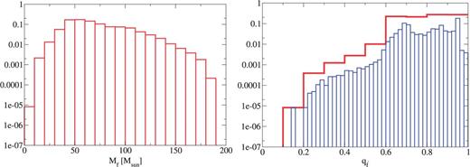
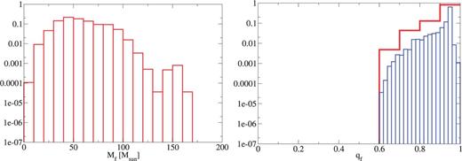
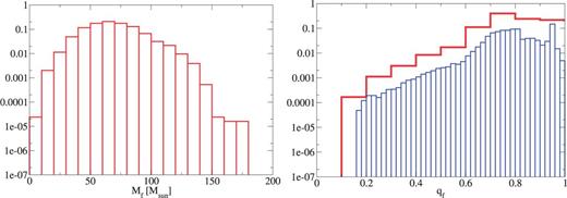
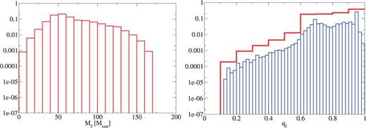
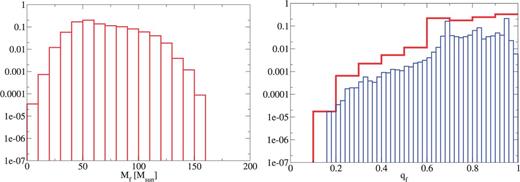
Based on Ref. [11] (see also Refs. [20,21]), we calculate the remnant mass and spin from given BH binary parameters, , , , and (see Ref. [4] for a detailed discussion). The remnant mass and spin for each case is shown in Figs. 16–25. Here, we have normalized the distribution, and used binning with for and (thick, red) and (thin, blue) for .
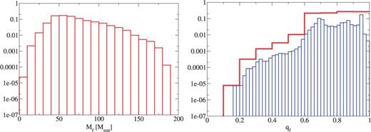
The remnant mass (left) and spin (right) for our standard model.
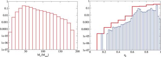
The remnant mass (left) and spin (right) for the IMF: logflat model.
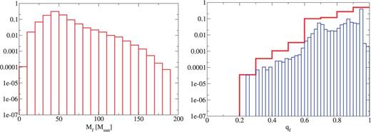
The remnant mass (left) and spin (right) for the IMF: Salpeter model.
The remnant mass (left) and spin (right) for the IEF: model.
The remnant mass (left) and spin (right) for the IEF: model.
The remnant mass (left) and spin (right) for the model.
The remnant mass (left) and spin (right) for the model.

The remnant mass (left) and spin (right) for the model.
The remnant mass (left) and spin (right) for the model.
The remnant mass (left) and spin (right) for the model.
The IMF dependence shown in Figs. 16, 17, and 18 is described below for the remnant mass and spin. When we treat the steeper IMF, we have a lower number of high-mass remnants. On the other hand, the number of high-spin remnants increases slightly in the steeper IMF cases. This is because in the steeper IMF models we have a large number of progenitors with mass smaller than .
As for the IEF dependence, we find that in Figs. 16, 19, and 20 there is no strong tendency.
Next, from Figs. 16, 21, 22, and 23 the CE parameter dependence can be described. In the model, the maximum of the remnant mass becomes much smaller than that of our standard model. This is because the high-mass progenitors merge during a CE phase due to too-small . As for the remnant spin, we do not have remnant spins which are smaller than since BBHs tend to be of equal mass. If a light BH falls into a non-spinning massive BH, the remnant BH can have a small spin (). However, in the above model many BBHs are equal mass. In the model, the maximum remnant mass is smaller than that of our standard model again. In this model, the fraction of remnant spins with is larger than that for our standard model because the fraction of group 3 in this model is larger than in our standard model.
As for the dependence, we find from Figs. 16, 24, and 25 that the maximum remnant mass becomes lower for higher , due to the mass loss during RLOF.
5.2. Event rates for ringdown gravitational waves
To estimate the event rate for ringdown gravitational waves, it is necessary to have the merger rate density of Pop III BBHs. The merger rate density has been derived for various models in Ref. [6], and can be approximated by a fitting formula for low redshift. This is summarized in Table 2. In practice, we have considered the fitting for in terms of redshift up to , but the above is derived by using where denotes the (luminosity) distance, because we use it only up to in this paper.
Fitting formulas of the merger rate density for low redshift in the center column. Here, denotes the (luminosity) distance. In the right column, the event rates divided by dependence on the star formation rate and the fraction of the binary are shown for each model. We consider events with for the KAGRA detector here.
| Model | ||
|---|---|---|
| Standard | 446 | |
| IMF: logflat | 255 | |
| IMF: Salpeter | 61.5 | |
| IEF: | 452 | |
| IEF: | 451 | |
| 5.87 | ||
| 146 | ||
| 372 | ||
| 499 | ||
| 158 |
| Model | ||
|---|---|---|
| Standard | 446 | |
| IMF: logflat | 255 | |
| IMF: Salpeter | 61.5 | |
| IEF: | 452 | |
| IEF: | 451 | |
| 5.87 | ||
| 146 | ||
| 372 | ||
| 499 | ||
| 158 |
In Fig. 26, based on Ref. [24], we show the parameter estimation in a case with for the typical case [5,6] (with and ). The (black) thick line shows the Schwarzschild limit and the ellipses are the contours of and . In general relativity, the top-left side of the thick black line is prohibited. Thus, using the event with , we summarize various event rates in Tables 3 and 4. Table 3 shows the total event rates divided by dependence on the star formation rate and the fraction of the binary for ten models, and those for a remnant BH with , , and .
![In the (fR,fI) plane, we show the parameter estimation in a case with SNR=35 for the typical case [5,6] (with Mrem=57.0904M⊙ and αrem=0.686710). The (black) thick line shows the Schwarzschild limit and the ellipses are the contours of 1σ, 2σ, 3σ, 4σ, and 5σ. In general relativity, the top-left side of the thick black line is prohibited.](https://oup.silverchair-cdn.com/oup/backfile/Content_public/Journal/ptep/2016/10/10.1093_ptep_ptw143/3/m_ptw143f26.jpeg?Expires=1750314340&Signature=bFu1zbdnZeFct5CMlE9I0HI7Wr2BpI5okFvZUOJEcWTWGO1HIONjxlmNj4CFGTMeyM5zi41uKbFxXH97~3g6aBJK2B4F-dr-CoSwZ3d5ghZWdHGbjjzimdOsb9GGSlREyMIuSYT1vxdVEHVzzs6nQNNKdQqly1auKQUEQlivvvjRpzwwCu4Bl7KD4H4rxOYw9QgSYDDXz2Jq-1Hzu-oQ2IZnHRdl9WcNjgX8U3aerAieN23Pd5gvJydwbgKC~eiYuSuuiRdz3ZWB8c08KMPkZEC1bF9fRflMxOy-4WiTgocZYu-RgvF2T0SInLNgja3hyY4FNVCq4iRRDrIDQCR1XQ__&Key-Pair-Id=APKAIE5G5CRDK6RD3PGA)
The total event rate divided by dependence on the star formation rate and the fraction of the binary for each model and those for the final , , and BHs in the case of for the KAGRA detector.
| Model | all | |||
|---|---|---|---|---|
| Standard | 3.73 | 2.45 | 0.115 | 0.0260 |
| IMF: logflat | 2.17 | 1.41 | 0.0659 | 0.0152 |
| IMF: Salpeter | 0.530 | 0.337 | 0.0153 | 0.00300 |
| IEF: | 3.80 | 2.38 | 0.0943 | 0.0248 |
| IEF: | 3.82 | 2.38 | 0.0800 | 0.0228 |
| 0.0463 | 0.0411 | 0.00832 | 0.00268 | |
| 1.23 | 0.864 | 0.0377 | 0.0114 | |
| 2.96 | 2.16 | 0.243 | 0.0372 | |
| 4.21 | 3.29 | 0.0981 | 0.0157 | |
| 1.58 | 0.705 | 0.0185 | 0.0128 |
The event rates divided by dependence on the star formation rate and the fraction of the binary as a function of the lower limit of the solid angle of a sphere , where the QNM is mainly emitted from the ergoregion, in the case of for the KAGRA detector.
| Model | ||||||
|---|---|---|---|---|---|---|
| Standard | 2.23 | 1.10 | 0.356 | 0.162 | 0.117 | 0.0780 |
| IMF: logflat | 1.29 | 0.621 | 0.207 | 0.102 | 0.0683 | 0.0454 |
| IMF: Salpeter | 0.309 | 0.145 | 0.0489 | 0.0234 | 0.0156 | 0.00960 |
| IEF: | 2.18 | 0.998 | 0.288 | 0.132 | 0.0955 | 0.0621 |
| IEF: | 2.15 | 0.936 | 0.237 | 0.115 | 0.0825 | 0.0518 |
| 0.0399 | 0.0318 | 0.0131 | 0.00966 | 0.00839 | 0.00503 | |
| 0.820 | 0.391 | 0.135 | 0.0609 | 0.0390 | 0.0222 | |
| 2.01 | 1.09 | 0.470 | 0.307 | 0.246 | 0.187 | |
| 3.09 | 0.979 | 0.294 | 0.127 | 0.0990 | 0.0292 | |
| 0.666 | 0.405 | 0.0278 | 0.0218 | 0.0187 | 0.0141 |
In Table 4, we present the detection rate divided by dependence on the star formation rate and the fraction of the binary as a function of the lower limit of the solid angle of a sphere by which we can estimate the contribution of the ergoregion. The relation between this and the spin parameter was obtained in Ref. [27] (see also the recent studies in [25,27,28,29]). It is noted that corresponds to .
6. Discussions
In this paper, we extended our previous work [4] (the standard model in this paper) by looking at the dependence on various parameters of the Pop III binary population synthesis calculation. As shown in the right column of Table 2, the detection rate with for the second-generation GW detectors such as KAGRA was obtained as 5.9–500 between ten models. Recently, Kushnir et al. [30] have discussed whether the BH's spin constrains the binary evolution path in the case of Pop I and Pop II binaries. If we detect a lot of Pop III BBH mergers, we might be able to constrain the Pop III binary evolution paths not only by the mass distribution but also by the spin distribution. In particular, as described in Sect. 4, the spin of a black hole depends strongly on whether the progenitor of black hole enters the CE phase or not. Thus, we can check whether a BBH progenitor evolved via the CE phase or not by the spins of the BBH.
One of the interesting outputs from the QNM GWs is whether we can confirm the ergoregion of the Kerr BH. From Table 4, the event rate for the confirmation of of the ergoregion is with .
Finally, Pop III BBH mergers can be a target for space-based GW detectors such as eLISA [34] and DECIGO [35]. Study in this direction is one of our future works.
Acknowledgements
This work was supported by MEXT Grant-in-Aid for Scientific Research on Innovative Areas, “New Developments in Astrophysics Through Multi-Messenger Observations of Gravitational Wave Sources,” Nos. 24103001 and 24103006 (HN, TN), JSPS Grant-in-Aid for Scientific Research (C), No. 16K05347 (HN), and Grant-in-Aid from the Ministry of Education, Culture, Sports, Science, and Technology (MEXT) of Japan No. 15H02087 (TN).
