


Abstract
Induced Compton scattering (ICS) is an interaction between intense electromagnetic radiation and plasmas, where ICS transfers the energy from photons to plasma. Although ICS is important for laser plasma interactions in laboratory experiments and for radio emission from pulsars propagating in pulsar wind plasmas, the detail of the photon cooling process has not been understood. The problem is that, when ICS dominates, the evolution of photon spectra is described as a nonlinear convection equation, which makes the photon spectra multi-valued. Here, we propose a new approach to treat the evolution of photon spectra affected by ICS. Starting from the higher-order Kompaneets equation, we find a new equation that resolves the unphysical behavior of photon spectra. In addition, we find the steady-state analytic solution, which is linearly stable. We also successfully simulate the evolution of photon spectra without artificial viscosity. We find that photons rapidly lose their energy by ICS with continuously forming solitary structures in frequency space. The solitary structures have the same logarithmic width characterized by an electron temperature. The energy transfer from photons to plasma is more effective for a broader spectrum of photons such as that expected in astrophysical situations.
1. Introduction
Nonlinear interactions between strong electromagnetic waves and plasmas have been studied in the context of laser plasma physics and astrophysical phenomena. Depending on intensities of radiation and conditions of plasmas, plenty of nonlinear interactions exist and are studied in different approaches. For example, quantum electrodynamics predicts vacuum-polarization effects, where photons interact with virtual electron–positron pairs (cf. Ref. [1]). Parametric processes in plasmas, such as induced scattering processes, filamentation instability, and so on have been studied in classical electrodynamics with the two-fluid description of plasmas (cf. Ref. [2]). There are also studies of parametric processes in the semi-classical formulation, which is used in this paper (cf. Refs. [3–5]). Here, we focus on induced Compton scattering (ICS), which is a parametric instability between photons and each electron, rather than plasmons. The condition for ICS to be dominant process is when both the central frequency and the spectral width of strong electromagnetic radiation are greater than the Langmuir plasma frequency [6]. ICS cools photons toward Bose–Einstein condensation, while plasmas are heated by this process (cf. Ref. [7]).
ICS has been studied in the context of laser plasma interaction both theoretically [8–10] and experimentally [11–14]. Most of these studied the process with the two-fluid approximation, which accounts only for the linear regime of the instability. On the other hand, ICS has also been studied for the scattering process around high intensity astrophysical sources with the semi-classical formulation, which can partly treat the nonlinear regime (e.g. Refs. [15–18]). However, these studies constrained plasma conditions around some astrophysical objects, considering only the scattering optical depth to ICS. It is known that there is a difficulty in treating the nonlinear regime of ICS even with the semi-classical formulation as described in this paper.
In the semi-classical formulation, a relaxation process of isotropic photons interacting with a rarefied Maxwellian plasma by Compton scattering is described by the Kompaneets equation [31]. The Kompaneets equation is the Fokker–Plank equation describing the evolution of a photon spectrum including the ICS term, which comes from the boson nature of photons, and which is quadratic in the intensity of the radiation. Therefore, for high intensity radiation, this quadratic term plays a dominant role and the Kompaneets equation is reduced to the nonlinear convection equation [Eq. (22)]. It is known that the nonlinear convection equation has an implicit solution, which will be multi-valued after a finite time starting from certain initial conditions. Such a spectrum is unphysical and should be modified to be single-valued, i.e., there should be an appropriate physical process which we have ignored (e.g. Ref. [19]).
Different approaches have been adopted to resolve the unphysical behavior of a photon spectrum when ICS dominates. Peyraud (1968) [20–22] considered heuristically adding a dispersive term (the third derivative term) to the nonlinear convection equation and made the equation a Korteweg–de Vries type, i.e., soliton formation in frequency space. Reinish (1976) [23, 24] considered recovering the diffusive term (the second derivative term), which is originally included in the Kompaneets equation, and made the equation Burgers type, which allows formation of a shock wave structure as in hydrodynamics. However, because the original diffusive term is linear in the intensity of radiation, this will not be applicable when the intensity of radiation becomes higher and higher. On the other hand, Zel’dovich and colleagues [25, 26] adopted the integral form of the equation, i.e., the Boltzmann equation [Eq. (1)]. They predicted formation of solitary structures in a radiation spectrum. It is worth distinguishing which spectral behaviors appear in a given condition between photons and electrons. There are also numerical studies of this problem by Montes (1977, 1979) [27, 28] and Coppi et al. (1993) [29]. We compare their results with ours in Sect. 4.3.
In this paper, we propose a new approach to studying the evolution of a radiation spectrum when ICS dominates. In Sect. 2, we extend the Kompaneets equation to the higher-order terms. This is in preparation for obtaining a new equation, and its derivation helps understand what the resolution of the problem in the nonlinear convection equation is. In Sect. 3, we find a new equation that describes the evolution of a spectrum for intense radiation. We obtain the analytic solution in steady state and also discuss its linear stability. In Sect. 4, we show some examples of numerical studies of the new equation. We give interpretations of our results and comparison with past studies. Section 5 is devoted to a summary.
2. Higher-order Kompaneets equation
Combining all of these, we obtain the higher-order Kompaneets equation that satisfies conservation of photon number, and the Bose–Einstein distribution is the equilibrium solution for this equation (cf. the study for Eq. (12), given by Caflisch and Levermore (1986) [33]). Note that the resultant equation is exactly the same as Eqs. (15) and (16) of Challinor and Lasenby (1998) [34], although they took a different approach to derive the equations.
3. The case for large occupation number: Steady-state solution and its stability
Note that Eq. (24) exactly corresponds to the isotropic case of Eq. (4) with |$\Delta S = 0$| and |$\Delta I = \Delta I_{(k)} + \Delta I_{(k p^2)}$|. In contrast to Eq. (22), the plasma temperature |$\Theta$| appears explicitly on the right-hand side that corresponds to |$\Delta I_{(k p^2)}$| [Eq. (18)]. Because the right-hand side is the higher-order correction term, the velocity of photon flux (in frequency space) is basically determined by the second term of the left-hand side, i.e., of order |$N(x)$| in the negative direction of |$x$|. The first term of the right-hand side is important in resolving the problem described in Sect. 1, while the second term slightly modifies the second term of the left-hand side. Equation (24) is similar to the Korteweg–de Vries equation, but the coefficient of the dispersive term is also nonlinear (proportional to |$N$|). This is different from the study by Peyraud (1968) [20–22].
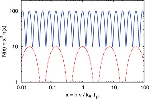
Plots of Eq. (26) in logarithmic scale for different parameters: |$(k_{\Theta }, A, B, \phi ) = (\pi , 5, 5, 0)$| (dotted red line) and |$(4 \pi , 45, 55, 0)$| (blue line). The plasma temperature of the blue line is colder than that of the red one.
4. Numerical simulation
Here, we numerically study the initial evolution of photon spectra by solving Eq. (24) with |$n \gg 1$|. We pay particular attention to evaluating the third derivative in Eq. (24) precisely in order to see the development of solitary structures as described by Zel’dovich and colleagues [25, 26].
4.1. Setup
Equation (24) is an approximated form of Eq. (23) for |$n \Theta \times \min (1, x) \gg 1$|. We checked that both of the equations give almost the same initial evolution until |$y \lesssim 0.4 y_0$| for the same parameter sets, satisfying |$n \Theta \times \min (1, x) \sim 10$| and |$10^2$| at the peak of the Gaussian |$x = x_{\rm init}$|. For |$0.4 y_0 \lesssim y \lt y_0$|, numerically unstable structures start to develop at the portion of |$N(x, y) \ll N_{\rm init}$| in our current scheme. This does not allow us to pursue the spectral evolution for different |$\sigma _{\rm init}$| and |$\lambda ^{}_{\rm \Theta }$| beyond |$y \sim 0.4 y_0$|. In what follows, we show numerical results of Eq. (24) for |$y \le 0.4 y_0$|. We fixed |$(N_{\rm init}, x_{\rm init}) = (10^7, 1)$|, since different sets of |$(N_{\rm init}, x_{\rm init})$| do not change the results as long as we measure |$y$| with |$y_0$|. For the remaining two parameters, we study the case that both |$\sigma _{\rm init}$| and |$\lambda ^{}_{\Theta }$| are of order |$10^{-1}$| (|$\lambda ^{}_{\Theta } = 0.1$| corresponds to an electron temperature of |${\sim }10^2$|eV).
Equation (24) has two invariants of motion, the photon number density |$\int N(x, y) dx$| and a quantity |$\int \ln N(x, y) dx$| [25]. Conservation of photon number is immediately found when we rewrite the |$x$| derivatives in Eq. (24) to the second line expression of Eq. (25) and integrate both sides of the equation over |${\textit {dx}}$|. We obtain conservation of the quantity |$\int \ln N(x, y) dx$| from dividing both sides of Eq. (24) by |$N(x)$| and integrating over |${\textit {dx}}$|. For all the results of our calculation below, we checked that these quantities were conserved for |$y \le 0.4 y_0$|.
4.2. Results
Figure 2 shows the results of the numerical simulations for different Doppler widths |$\lambda ^{}_{\Theta } = 0.20$|, |$0.10$|, and |$0.05$| where the initial spectral widths are |$\sigma _{\rm init} = 0.2$| for the left panel and |$\sigma _{\rm init} = 0.1$| for the right panel, respectively. Dotted black lines in Fig. 2 show the initial spectra |$N_0(x)$|, and thin red and thick blue lines are photon spectra |$N(x, y)$| at |$y = 0.2 y_0$| and at |$y = 0.4 y_0$|, respectively. We find that solitary structures are formed intermittently and shift to lower frequency, i.e., the direction of their motion is basically determined by the left-hand side of Eq. (24) and their solitary form results from the first term of the right-hand side of Eq. (24). The heights of each solitary structure increase with time without changing their logarithmic width. The smaller the value of |$\lambda ^{}_{\Theta }$|, i.e., the colder the plasma, the more and the narrower solitary structures are formed. This behavior is consistent with what is inferred from the steady-state solution [Eq. (26)]. On the other hand, numerical simulations without the third derivative in Eq. (24) give an unstable shock-like discontinuous structure rather than solitary structures with the use of the same scheme.
![Each panel shows results of numerical calculation of Eq. (24) for three different Doppler widths $\lambda _{\Theta } \equiv 2 \pi /k_{\Theta } = 0.20$ (uppermost lines), $0.10$ (middle lines), and $0.05$ (lowermost lines). The initial spectral widths are different between the left $(\sigma _{\rm init} = 0.2)$ and right panels $(\sigma _{\rm init} = 0.1)$, while $(N_{\rm init}, x_{\rm init}) = (10^7, 1)$ is common [see Eq. (29)], i.e., $y_0 = 10^{-7}$ for all cases. Dotted black, thin red, and thick blue lines correspond to $N(x, 0)$, $N(x, 0.2 y_0)$, and $N(x, 0.4 y_0)$, respectively. The insets are zooms of the solitary structures appearing in the middle line $(\lambda _{\Theta } = 0.10)$ and the lowermost line $(\lambda _{\Theta } = 0.05)$ in the left panel and in the lowermost line $(\lambda _{\Theta } = 0.05)$ in the right panel when $y = 0.4 y_0$. Thick blue lines in the insets are the results of calculation of $N(x, 0.4 y_0)$, and dotted yellow lines are Eq. (30) with parameters as tabulated in Table 1. The numbering of the solitary structures corresponds to the number $i$ in Table 1.](https://oup.silverchair-cdn.com/oup/backfile/Content_public/Journal/ptep/2015/7/10.1093_ptep_ptv086/3/m_ptv08602.jpeg?Expires=1750284252&Signature=nGQOO2Jicdd1WX8~EpI9BV5jtDADvus7eOzr~5MDpgtIihNqUyfYO~E8QKr5gBa9-m1XW8mS5JScDxSr9LmTdcv0dZFK43PNE1xvcKTCpxLIJ60HIhfb62OEP-FqlcAe5SaOQSXq~XKoqt8MlHrdurCh6uVovWZOEPBOSztOVQ3IhSK1O4sPMdL07uNHZUImFeINp3p1c4-q~1cvuRdEpIl89NHSZ9hR29RUILL3oQa7yoLDQkskoO2U6kx2Tm7Gr6Y5k26Fslo4JYIsO5YQ~WN0bgF0XIDc7ZNtcjGNKenoSObr~Dqj70NlwL0V~xCTJvKPhlVyKjs0OokqTh~brA__&Key-Pair-Id=APKAIE5G5CRDK6RD3PGA)
Each panel shows results of numerical calculation of Eq. (24) for three different Doppler widths |$\lambda _{\Theta } \equiv 2 \pi /k_{\Theta } = 0.20$| (uppermost lines), |$0.10$| (middle lines), and |$0.05$| (lowermost lines). The initial spectral widths are different between the left |$(\sigma _{\rm init} = 0.2)$| and right panels |$(\sigma _{\rm init} = 0.1)$|, while |$(N_{\rm init}, x_{\rm init}) = (10^7, 1)$| is common [see Eq. (29)], i.e., |$y_0 = 10^{-7}$| for all cases. Dotted black, thin red, and thick blue lines correspond to |$N(x, 0)$|, |$N(x, 0.2 y_0)$|, and |$N(x, 0.4 y_0)$|, respectively. The insets are zooms of the solitary structures appearing in the middle line |$(\lambda _{\Theta } = 0.10)$| and the lowermost line |$(\lambda _{\Theta } = 0.05)$| in the left panel and in the lowermost line |$(\lambda _{\Theta } = 0.05)$| in the right panel when |$y = 0.4 y_0$|. Thick blue lines in the insets are the results of calculation of |$N(x, 0.4 y_0)$|, and dotted yellow lines are Eq. (30) with parameters as tabulated in Table 1. The numbering of the solitary structures corresponds to the number |$i$| in Table 1.
Fitted values of |$n_i$| and |$m_i$| in Eq. (30). The number |$i$| of the solitary structures is found in the insets in Fig. 2. Corresponding |$\sigma _{\rm init}$| and |$\lambda ^{}_{\Theta }$| are also tabulated. |$\Delta m_i$| is the separation between the neighboring peaks of the |$i$|th solitary structure: |$\Delta m_{\rm 1a} = m_{\rm 2a} - m_{\rm 1a}$|, for example.
| |$i$| | |$\sigma _{\rm init}$| | |$4 w = \lambda ^{}_{\Theta }$| | |$n_i$| | |$m_i$| | |$\Delta m_i$| |
|---|---|---|---|---|---|
| 1a | 0.20 | 0.10 | |$3.42 \times 10^7$| | |$-$|0.869 | 0.192 |
| 2a | |$2.38 \times 10^7$| | |$-$|0.677 | 0.173 | ||
| 3a | |$1.38 \times 10^7$| | |$-$|0.504 | 0.153 | ||
| 4a | |$4.78 \times 10^6$| | |$-$|0.351 | — | ||
| 1b | 0.20 | 0.05 | |$3.64 \times 10^7$| | |$-$|0.921 | 0.0996 |
| 2b | |$3.14 \times 10^7$| | |$-$|0.821 | 0.0960 | ||
| 3b | |$2.64 \times 10^7$| | |$-$|0.725 | 0.0915 | ||
| 4b | |$2.16 \times 10^7$| | |$-$|0.634 | 0.0873 | ||
| 5b | |$1.68 \times 10^7$| | |$-$|0.547 | 0.0838 | ||
| 6b | |$1.15 \times 10^7$| | |$-$|0.463 | 0.0795 | ||
| 7b | |$6.27 \times 10^6$| | |$-$|0.383 | — | ||
| 1c | 0.10 | 0.05 | |$3.30 \times 10^7$| | |$-$|0.481 | 0.0981 |
| 2c | |$2.44 \times 10^7$| | |$-$|0.383 | 0.0917 | ||
| 3c | |$1.68 \times 10^7$| | |$-$|0.292 | 0.0844 | ||
| 4c | |$9.40 \times 10^6$| | |$-$|0.207 | — |
4.3. Discussion
Radio emissions from pulsars (e.g., Ref. [37]) and also fast radio bursts (e.g., Refs. [41]) have extremely large brightness temperatures. Although the optical depth to ICS |$\tau _{\rm ind}$| would tend to unity for these objects (cf. Refs. [15, 16, 18]), the past studies did not discuss what kind of signatures are expected to be imprinted in their observed spectra. Our present study predicts a spectral break at the frequency |$\nu _{\rm ind}$| corresponding to |$\tau _{\rm ind}(\nu _{\rm ind}) \gtrsim 0.2$| and solitary structures below |$\nu _{\rm ind}$| in the photon spectra (thin red lines in Fig. 2). In this regard, the discrete emission bands in the dynamic spectra of the giant radio pulse occurring in the interpulse phase of the Crab pulsar reported by Hankins and Eilek [37] (“zebra bands”) are intriguing phenomena. If we interpret their reported value |$\Delta \ln \nu = \Delta \nu / \nu \sim 0.06$| by ICS, the value is not far from |$\Delta m_i$| for |$\lambda ^{}_{\Theta } = 0.05$| in Table 1, corresponding to an electron temperature of |$\sim$| a few |$\times 10$|eV. However, for applications to realistic astrophysical situations, we should take account of anisotropic photon distributions and relativistic effects of both bulk and thermal motions of plasmas. These effects will be studied in subsequent papers.
Figure 3 plots the evolution of the normalized photon energy density with time for the results of Fig. 2. We also show the case for an initial width of |$\sigma _{\rm init} = 0.05$| as dotted lines in Fig. 3. Thin lines (|$\sigma _{\rm init} = 0.20$|) show the exponential energy loss, although the slope is not exactly |$\ln [\epsilon _{\rm ph}(y) / \epsilon _{\rm ph}(0)] = -y/y_0$|. Thick (|$\sigma _{\rm init} = 0.10$|) and dotted (|$\sigma _{\rm init} = 0.05$|) lines deviate from the exponential law (thin lines) at |$y \sim 0.15 y_0$| and |$y \sim 0.05 y_0$|, respectively. The dotted red line |$(\sigma _{\rm init}, \lambda _{\Theta }) = (0.05, 0.10)$| and thick black line |$(\sigma _{\rm init}, \lambda _{\Theta }) = (0.10, 0.20)$| show a slightly different slope even at |$y \lesssim 0.05 y_0$| from the other lines and these exceptional behaviors are characterized by a relatively large Doppler wavelength |$\lambda _{\Theta } = 2 \sigma _{\rm init}$|, which will be discussed later in this section. The energy transfer from photons to plasma by ICS is more effective for the case of broad initial spectra than narrow ones (the blue lines are always below the red lines for the same |$\sigma _{\rm init}$|). This means that the deviation of |$N(x, y)$| from the initial spectrum |$N_0(x)$| is faster for narrower spectra and this behavior is found from the inset in the right panel of Fig. 2 (the thick blue line is well below the dotted yellow line compared with those in the left panel of Fig. 2). Although we see a temperature dependence of the energy transfer for the same initial width, Eq. (31) has no information of electron temperature explicitly. The third derivative in Eq. (24) may act as a heating term because larger |$\lambda _{\Theta }$| (higher temperature) gives slower energy transfer in Fig. 3. This is consistent with the discussion at the steady-state solution Eq. (26), i.e., the photon flux is written as |$\approx B^2 - A^2$| for |$\Theta \ll 1$| and a contribution from |$\Delta I_{(k p^2)}$| (|$A$|) resists that from |$\Delta I_{(k)}$||$(B)$|.
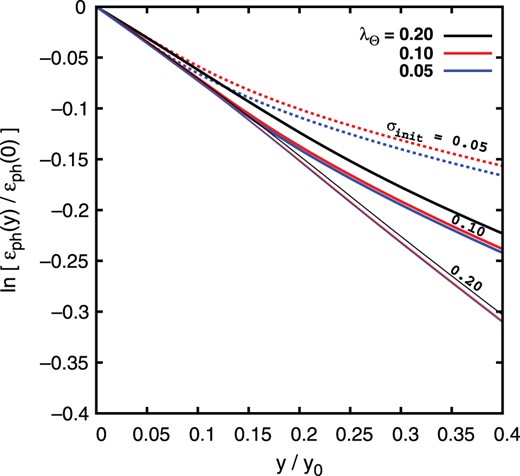
Evolution of the normalized photon energy density |$\epsilon _{\rm ph}(y)/\epsilon _{\rm ph}(0)$| with the normalized time |$y/y_0$|. The vertical axis is the natural logarithm of |$\epsilon _{\rm ph}(y)/\epsilon _{\rm ph}(0)$|. Thick and thin lines correspond to |$\sigma _{\rm init} = 0.20$| (left panel in Fig. 2) and |$= 0.10$| (right panel in Fig. 2). We also show the results for |$\sigma _{\rm init} = 0.05$| (dotted lines) for two different Doppler widths of |$\lambda ^{}_{\Theta } = 0.10$| (red) and |$0.05$| (blue), respectively.
We should note the case of |$\lambda _{\Theta } = 2 \sigma _{\rm init}$|, i.e., the full width of the initial spectrum is almost the same as the Doppler width. For |$\lambda _{\Theta } >2 \sigma _{\rm init}$|, evolution of photon spectra is unstable, at least in our numerical scheme. In those calculations, although all of the results shown in this paper have no time variation of |$N(x >x_{\rm init}, y)$| (see Fig. 2), there appear unstable features at |$x \gtrsim x_{\rm init}$| for |$\lambda _{\Theta } >2 \sigma _{\rm init}$|. This unstable feature is not improved by higher numerical resolutions of both |$x$| and |$y$|. Currently, it is uncertain whether the exceptional behaviors of the dotted red line |$(\sigma _{\rm init}, \lambda _{\Theta }) = (0.05, 0.10)$| and thick black line |$(\sigma _{\rm init}, \lambda _{\Theta }) = (0.10, 0.20)$| in Fig. 3 are numerical or physical. However, we should also take care of our formulation [Eq. (1)] for a narrow spectrum |$\sigma _{\rm init} \ll \lambda _{\Theta }$|. Galeev and Syunyaev (1973) [6] argued that, when |$\sigma _{\rm init} \ll \lambda _{\Theta }$|, collective behaviors of plasmas are more important than the interaction with free electrons, i.e., Compton scattering. This is the reason why we do not study the case for |$\lambda ^{}_{\Theta } >2 \sigma _{\rm init}$| more in this paper, although study of this regime is important for application to laboratory experiments.
We finally discuss differences from past calculations of spectral evolution by ICS [28, 29]. Figure 1 of Coppi et al. (1993) [29] shows spectral evolution for the isotropic case. Basically, they solved Eq. (22) but including numerical viscosity, i.e., their calculations did not have information of plasma temperature |$(\lambda _{\Theta })$|. Although their result (the right panel of Fig. 1 of Coppi et al. (1993) [29]) showed two solitary structures that have the same logarithmic width, their behaviors seem different from ours, such as the height of the low frequency structure is smaller than that of the high frequency one. We consider that these structures are numerical, i.e., a combination of the numerical viscosity and logarithmically spaced frequency grids in their calculations. Montes (1979) [28] solved the integro-differential equation given by Zel’dovich et al. (1972) [26], but with some simplifications. Figure 2 of Montes (1979) [28] (the calculation for an initially broad Gaussian spectrum) shows solitary structures of the linearly same width. We consider that Eq. (27) of Montes (1979) [28] is oversimplified; in particular, their assumption |$\Delta \nu \approx \Theta ^{1/2} \nu _0 =$| const. in their Eq. (20) is crucial, while we consider the case |$\Delta \nu \approx \Theta ^{1/2} \nu$| [25].
5. Conclusions
In this paper, we study evolution of photon spectra when ICS dominates. To get rid of the well-known difficulty of the nonlinear convection equation [Eq. (22)], we consider the higher-order Kompaneets equation. We obtain the new equation [Eq. (24)] that describes the evolution of the photon spectrum by ICS and that overcomes the difficulty. The second-order induced term |$\Delta I_{(k p^2)}$| [Eq. (18)] obtained from the higher-order Kompaneets equation improves the formulation. In addition, Eq. (24) has a steady-state analytic solution [Eq. (26) and Fig. 1], which is linearly stable. The steady-state analytic solution predicts the formation of solitary structures of the same logarithmic width in frequency space and the |$\Delta I_{(k p^2)}$| term acts as a heating term against the ICS term |$\Delta I_{(k)}$|, which is the pure cooling term.
We also study the evolution of photon spectra by ICS numerically. ICS intermittently forms solitary structures moving toward lower frequency (Fig. 2) and these behaviors are consistent with predictions by some previous studies [25, 26]. The solitary structures have the same logarithmic width well characterized by the Doppler width |$\lambda _{\Theta }$|, and this behavior is also inferred from the steady-state solution. On the other hand, the spacing between the peak frequencies of the structures does not follow Eq. (24) |$(\Delta m_i \ne \lambda _{\Theta })$|. The number and height of the solitary structures depend on |$\lambda _{\Theta }$|.
The results of our numerical simulation satisfy the two invariants of motion, conservation of photon number |$\int N(x) dx$| and of the quantity |$\int \ln N(x) dx$|. On the other hand, the energy density of photons |$\int x N(x) dx$| is transferred to electrons (Fig. 3). Energy density decays exponentially in the initial phase and this behavior is almost consistent with the analytic estimate [Eq. (31)]. The energy transfer from photons to plasmas by ICS is effective for the case of broad initial spectra such as expected in astrophysical situations. The numerical results shown in the present paper are only the initial phases of evolution |$y \le 0.4 y_0$|. We need a more optimized numerical scheme to study evolution for |$y >0.4 y_0$|.
Acknowledgements
S.J.T. would like to thank Y. Ohira, R. Yamazaki, Y. Sakawa, and F. Takahara for useful discussions. We would also like to thank the anonymous referee for his/her helpful comments. This work is supported by JSPS Research Fellowships for Young Scientists (S.T., 2510447).
