


Abstract
The International Linear Collider (ILC) is a next-generation accelerator for high-energy physics to study the Higgs sector in the Standard Model in as much detail as possible and to search for new phenomena beyond the Standard Model, such as supersymmetry and dark matter. In the current design of the positron source for the ILC, positrons are generated by pair creation in a Ti (titanium) alloy target via gamma irradiation. The gamma rays are generated by undulator radiation with electrons at more than 150 GeV. This positron generation scheme is an unprecedented approach; therefore, it is desirable to have a technical backup for the ILC positron source. We study a positron source for the ILC based on the conventional electron-driven scheme. In this scheme, a positron beam is generated by an electron beam of several GeV impinging on a W–Re (tungsten rhenium) alloy target. The heavy heat load and target destruction are potential problems, but they are alleviated by stretching the effective pulse length to 60 ms instead of 1 ms. In this article, a start-to-end simulation of the electron-driven ILC positron source is reported. According to the simulation, sufficient positrons can be generated while the target heat load is kept below the destruction threshold.
1. Introduction
The International Linear Collider (ILC) is an |$e^{-}$| and |$e^{+}$| linear collider for high-energy physics with a center-of-mass energy of 500 GeV (first phase) and 1 TeV (second phase). Compared to a proton collider such as the Large Hadron Collider (LHC), the ILC can make high-precision measurements because events can be fully reconstructed, the electrons (optionally, positrons) are polarized, and there are far fewer background events than in the LHC. Therefore, the ILC will reveal new physics behind electroweak symmetry breaking by precise measurements of the Higgs sector, top quark, and so on [1–3]. The ILC is also highly sensitive to physics beyond the Standard Model, such as supersymmetry, dark matter, and extra dimensions [1–3].
The ILC consists of an electron source, a positron source, damping rings (DR), the main linac, the final focus system, and detectors. The 500 GeV ILC design has several parameter sets. The two main sets are the high-luminosity and nominal sets. Here, the high-luminosity set is shown, and the nominal set appears in parentheses. A luminosity of |$3.6 (1.8) \times 10^{34}\,{\rm cm}^{-2}\,{\rm s}^{-1}$| is realized by collisions with an extremely small beam spot (5 nm in the vertical direction at the interaction point) and a high bunch intensity (3.2 nC). The 0.96 (0.72) ms beam pulse contains up to 2625 (1312) bunches, and the pulse is repeated at 5 Hz. The number of particles per second is roughly 50 times that of the Stanford Linear Collider (SLC), which was the first linear collider [4]. In the ILC Technical Design Report published in 2013 [1], this large amount of positrons is generated by an undulator scheme as the baseline. High-energy gamma rays are generated by undulator radiation. The gamma rays are converted to positrons through pair-creation processes in a Ti (titanium) alloy target. For efficient positron generation, the gamma ray energy has to be more than 10 MeV, which requires a 150 GeV driving electron beam with a 10 mm undulator period. Therefore, the high-energy electron beam is shared by the undulator and |$e^{+}$| and |$e^{-}$| collisions. This undulator positron generation has never been in operation for an accelerator, and any system demonstration is practically difficult. Although there are no fundamental difficulties with undulator positron generation, a technical backup is desirable to mitigate unknown technical risks.
As the technical backup, two schemes have been proposed, an electron-driven scheme and a Compton scheme. High-energy photons can be obtained more easily in the Compton scheme than in the undulator scheme because the wavelength of the solid-state laser is much shorter than the period of the undulator. However, it is still not easy to generate sufficient photons because the cross section is small. The Compton scheme has been studied in Refs. [5, 6] and developed in Refs. [7, 8] at KEK's Accelerator Test Facility. Although the number of generated photons has been increased, it is still not sufficient for the ILC positron source, and the scheme is not feasible as the technical backup.
In a conventional source, an electron beam of several GeV impinges on a heavy metal target. Through the Bremsstrahlung process, many gamma rays are emitted by the electrons and immediately converted to positrons through pair creation. For example, the conventional source was employed by the KEKB [9] linac, which generated positrons by a 4 GeV electron beam impinging on tungsten–copper or tungsten single-crystal [10, 11]. In this scheme, the positrons cannot be polarized. Experience at the SLC indicates that the peak energy deposition density (PEDD) in the target has to be less than 35 J/g [12–14] to avoid any damage to the target. The PEDD is the maximum energy deposition per volume (J/cm|$^3$|) normalized with the material density (g/cm|$^3$|).
An electron-driven positron source for the ILC was considered in Ref. [15], which reports that this method incurs a technical risk with respect to the heat load of the production target. It was pointed out in the report that the target has to be rotated at a tangential speed of 400 m/s in vacuum to mitigate the risk, which introduces other technical risks. To avoid the need for rapid rotation by relaxing the heat load, positron pulse stretching and beam size enlargement have been proposed by Omori et al. [16]. In this method, positrons are generated in 63 ms instead of 1 ms, and the heat load is reduced by a factor of 60. The electron-driven positron source for ILC can be accommodated in the tunnel designed for the undulator positron source, because the tunnel is wide enough. The compatibility of both schemes is one of the hottest topics in the LCC (Linear Collider Collaboration) [17].
To determine the target speed, the positron production condition has to be evaluated reliably. The positron yield is determined as the number of produced and captured positrons per electron. Once the yield is obtained, the electron intensity to obtain the required positrons is determined, and the PEDD can be calculated. In Ref. [16], the yield has been estimated by a simulation up to 250 MeV, where the capture linac ends. To improve the accuracy of the yield estimation, a start-to-end simulation has to be conducted, i.e., a simulation up to 5.0 GeV that includes a chicane, a positron booster up to 5.0 GeV, and an energy compressor section (ECS). In addition, the dynamic aperture (acceptance) of the DR in longitudinal and transverse phase space should be properly accounted for.
In this paper, we report a start-to-end simulation of the ILC positron source driven by an electron beam. In this simulation, all the components from positron generation to injection to the DR are included to obtain the positron yield. By studying the yield as a function of various conditions, the system is optimized, and the requirements for each component, such as the target, adiabatic matching device (AMD), capture linac, booster linac, and ECS, are clearly defined. Once the yield is properly calculated, the PEDD on the target is estimated for positron generation for the ILC. If the PEDD is below the threshold, the electron-driven scheme can be a technical backup for the ILC positron source.
In the following sections, the electron-driven positron source and start-to-end simulation are described. Finally, we present an optimized positron source configuration as our summary.
2. Electron-driven positron source
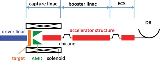
Schematic layout of the ILC electron-driven positron source.
2.1. Pulse structure and positron generation
The electron beam energy and bunch intensity of the driver linac are typically 6.0 GeV and |$2.0\times 10^{10}$|, respectively. The target is typically a 14 mm thick W–Re (tungsten rhenium) alloy, which corresponds to a 4.0 radiation length for efficient conversion and high robustness [18]. One positron generation pulse lasts for 63 ms. During the 63 ms duration, 20 RF pulses are fired at 300 Hz; each RF pulse duration is 1.0 |$\mu {\rm s}$|. Each RF pulse contains |$3\times 44$| bunches in the form of a triplet of mini-trains. One mini-train contains 44 bunches with a 6.15 ns spacing, and the mini-train interval is 100 ns. The triplet format is compatible with the bunch fill pattern in the DR, and the triplet pulse is injected to the DR without any bunch-by-bunch manipulation. The 100 ns spacing is necessary to prevent electron cloud instability in the DR. The average beam current of the pulse is about 0.5 A, and we employ a normal-conducting (NC) RF system to provide acceleration.
To evaluate the PEDD on the target, 132 bunches in a triplet are considered to impinge on the same spot because the target motion during the duration (in total 1 |$\mu $|s) is on the order of several |$\mu $|m if the target's tangential speed is on the order of several meters per second. On the other hand, the 3.3 ms RF pulse interval corresponds to several millimeters or centimeters in the target position, and it significantly contributes to the heat load reduction. According to the studies in Ref. [16], an electron beam with a 6.0 GeV energy, |$2.0\times 10^{10}$| bunch intensity, and 4.0 mm beam spot in RMS yields a PEDD of 23 J/g for a 14 mm thick W target, which is below the practical limit of 35 J/g. The W and W–Re targets have almost the same properties, except for stress durability; therefore, these PEDD values should be almost the same. During the 3.3 ms triplet interval, the target is moved by 16.5 mm, assuming a 5 m/s target speed. Because this number is more than the |$4 \sigma $| value of the beam spot and the overlap is less than 10%, the effect of the overlap is limited.
2.2. Adiabatic matching device
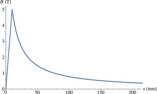
AMD magnetic field along the longitudinal position. From |$s=0$| to the peak (|$s=10$| mm), the field increases linearly. At |$s\geq 10$| mm, the field is given by Eq. (2) (|$z=s-10$| mm). The target ends at |$s= 5$| mm.
2.3. Capture linac
The capture linac consists of 1.3 GHz L-band NC accelerators having an aperture radius and accelerator gradient of 20 mm and 25 MV/m, respectively. An L-band accelerator having an aperture 46 mm in radius and a 12 MV/m accelerator gradient with a 10 MW input power was designed by Argonne National Laboratory's Wakefield Accelerator facility (US) [23], and our working assumptions regarding the L-band accelerator are reasonable. The ILC capture linac accelerates the beam to 250 MeV with a 0.5 T solenoid field. The target, AMD, and accelerator structure are surrounded by the solenoid, as shown in Fig. 3. Not only positrons but also electrons are generated from the target. Because the electrons have an opposite electrical charge, at the entrance of the first RF cavity, the positrons and electrons on the same RF phase make opposite contributions and the total beam-loading effect is reduced by the cancellation. After significant deceleration to the electrons (or positrons) and the RF phase slippage, both the electrons and positrons are on each acceleration phase. From the end of the first RF cavity, the beam loading becomes twice that by the positrons. They are captured by the capture linac on the reverse RF phase. Then, the electrons provide beam loading with the same sign as that provided by the positrons. Therefore, the beam loading becomes twice that provided by the positrons. Our simulation omits any beam-loading effects, which are an issue for future work.
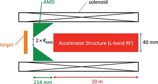
Schematic layout of the capture linac.
2.4. Chicane
After the capture linac, a chicane section is placed to remove positrons with a large energy deviation and electrons in order to reduce the beam-loading effect after the chicane and to avoid radiation activity caused by the loss of the beam, which passes through the booster linac with a high energy and a large energy deviation. The chicane can also eliminate photons generated by the target. From this viewpoint, the chicane should be upstream. On the other hand, the positron capture efficiency will be affected if the chicane is placed in the lower-energy region, because the positron beam still has a large energy deviation and large beam size. In our simulation, the chicane is placed after the capture linac, where the beam energy is 250 MeV. Figure 4 shows the beta and dispersion functions in the chicane section. The horizontal axis shows the distance from the entrance of the chicane section. The image at the bottom shows the magnet lattice. At the entrance of the chicane section, the typical geometrical horizontal and vertical RMS emittances are 18 |$\mu $|m.
Beta function (top) and dispersion function (middle) in the chicane section. The solid and dashed lines show horizontal and vertical values, respectively. The horizontal axis shows the distance from the entrance of the chicane section (m). The image at the bottom shows the magnet lattice; yellow, green, and blue rectangles show a bending magnet, quadrupole magnet, and RF cavity, respectively.
2.5. Booster linac
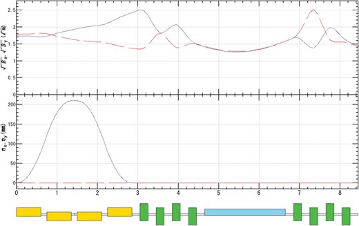
Positrons are accelerated by the booster linac up to 5 GeV from 250 MeV. Figure 5 shows the beta and dispersion functions in the booster linac including the chicane. The booster linac, which consists of 118 RF cavities, contains three types of lattice cells. In the first 6 lattice cells, each cell consists of four quadrupoles and one RF cavity. In the next 12 lattice cells, each cell consists of four quadrupoles and two RF cavities. In the next 22 lattice cells, each cell consists of four quadrupoles and four RF cavities. All of the RF cavities in the booster linac are 2 m in length. To suppress beam loss by the accelerator aperture, the upstream lattice cells have a large density of quadrupole magnets to keep the beam size small enough compared to the aperture owing to the small beta function. Because of the adiabatic damping, the beta function can be large downstream of the booster linac to obtain the same beam size. At the end of the booster section, the typical geometrical horizontal and vertical RMS emittances are 0.8 |$\mu $|m and the transmitted ratio (the number of transmitted particles at the entrance of the booster divided by that at the end of the booster) is 0.84.
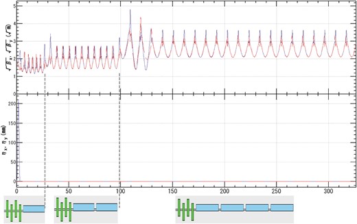
Beta function (top) and dispersion function (middle) in the chicane and booster. The solid and dashed lines show horizontal and vertical values, respectively. The horizontal axis shows the distance from the entrance of the chicane section (m). The bottom image shows the base structure of the magnet lattice; green and blue rectangles show a quadrupole magnet and RF cavity, respectively.
For a higher yield, an L-band accelerator driven by a high-power RF source is ideal because of the large aperture, but such a system could be expensive. The S-band is more cost effective, but the yield could be limited by the small aperture. As a compromise, the positron booster is a hybrid containing both L-band and S-band accelerators, as explained in detail in the next section.
2.6. Energy compression system
The ECS is placed after the booster linac for energy compression. The DR acceptance for |$\delta $| is narrower than that for |$z$| because the relative energy spread due to RF curvature, assuming L-band or S-band acceleration with a 75 mm bunch length, is much larger than 1.5%. Longitudinal phase-space rotation by the ECS increases the yield by better matching to the DR acceptance. Figure 6 shows the beta and dispersion functions in the ECS section. At the end of the ECS section, the typical geometrical horizontal and vertical RMS emittances are 0.8 |$\mu $|m and the transmitted ratio (the number of transmitted particles at the entrance of ECS divided by that at the end of ECS) is 0.97.
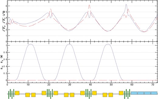
Beta function (top) and dispersion function (middle) in the ECS section. The solid and dashed lines show horizontal and vertical values, respectively. The horizontal axis shows the distance from the entrance of the ECS section (m). The bottom image shows the magnet lattice; yellow, green, and blue rectangles show a bending magnet, quadrupole magnet, and RF cavity, respectively.
Figure 7 shows the allowed energy spread before the booster linac (vertical axis) as a function of the bunch length (horizontal axis). In this calculation, the energy spread |$\delta $| at the end of the capture linac and the spread due to the RF curvature in the booster linac are added linearly for simplicity. Both axes indicate the full width about the bunch length and energy spread. The areas below the solid and dashed lines correspond to the allowed regions for the S-band and L-band boosters, respectively. For example, if the captured positron bunch in the capture linac has an energy spread of 200 MeV and a |$z$| value of 10 mm, it can be accepted by the DR after ECS phase-space rotation with S- or L-band acceleration. In the ECS, |$R_{56}$| is 1 m or less. From this viewpoint, both the S-band and the L-band are acceptable for the booster; however, the first half should be L-band and the last half can be S-band because of the transverse aperture, which is discussed in the next section.
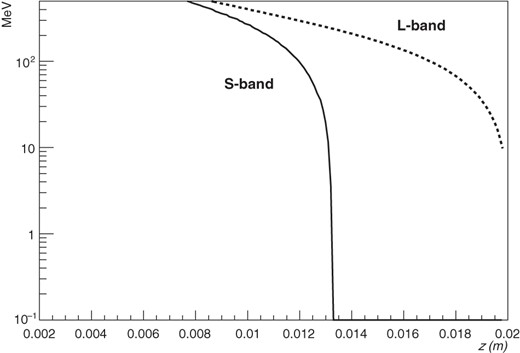
Allowed region of energy spread and bunch length at the end of the capture linac. The L- and S-bands are usable below the dashed and solid lines, respectively.
3. Positron capture simulation
The results of the start-to-end simulation of positron generation are presented in this section. Positrons generated by electron injection to the W target are simulated by GEANT4 [25]. The particles are generated as described in Ref. [16]. One thousand electrons are impinged on the target, and 12 700 positrons are obtained. The data are imported to the general particle tracer [26] to perform the tracking simulation from the target to the end of the capture linac. From the chicane to the end of the ECS, the particle tracking is simulated by the Strategic Accelerator Design program [27].
3.1. Typical positron distribution
Figures 8 and 9 show the positron distributions before (crosses) and after (triangles) the chicane section in the transverse plane (|$x$|–|$y$|), and Fig. 10 shows those in longitudinal phase space (|$z$|–|$\delta $|). In Figs. 8 and 9, the accelerator aperture of the booster linac is indicated by the red circle as a reference. The chicane increases the horizontal beam size once by dispersion, but it is focused down before the entrance of the booster linac, as shown in Fig. 4. The chicane improves the capture efficiency slightly because of the phase-space modulation by the chicane, as shown in Fig. 10, and the acceleration acts as an energy compressor.
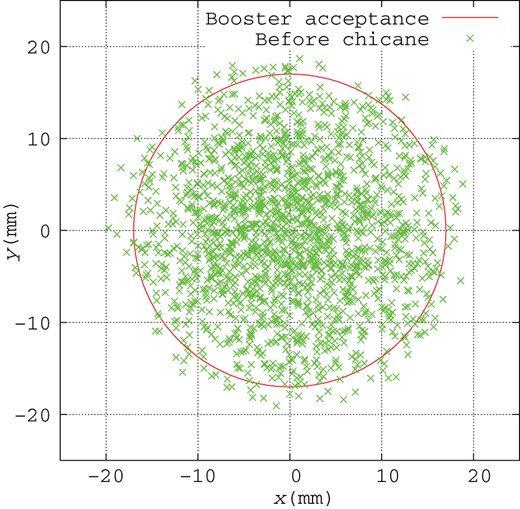
Positron distribution in transverse space with 17 mm circle at the end of the capture linac (crosses), where the beam energy is 250 MeV.
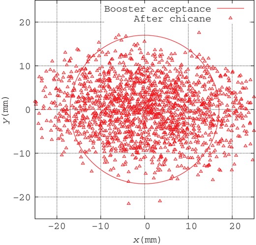
Positron distribution in transverse space with 17 mm circle at the end of the chicane (triangles), where the beam energy is 250 MeV.
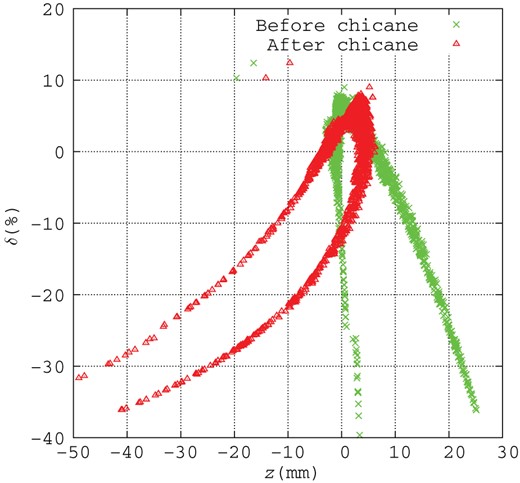
Positron distribution in longitudinal phase space at the end of the capture linac (crosses) and chicane (triangles).
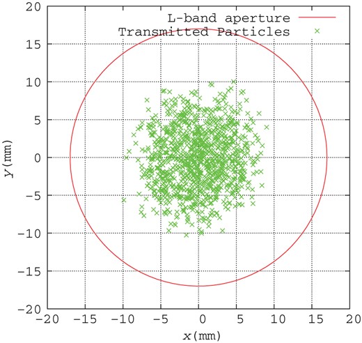
Figure 11 shows the positron distribution in the transverse plane at the end of the booster linac, where the beam energy is 5.0 GeV. In this subsection, only the L-band accelerator structure is used in simulation. Crosses show positrons passing through the booster linac. The transverse beam size is compressed by acceleration and is less than the radius of the S-band aperture (10 mm), which is indicated by the circle in Fig. 11. Figure 12 shows the positron distribution in longitudinal phase space at the end of the booster linac. Energy modulation due to RF curvature of the L-band acceleration appears, and the relative momentum deviation |$\delta $| remains large. This is one of the largest differences from the results in Ref. [16], which did not account for any effects of the booster linac.
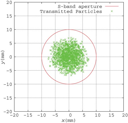
Positron distribution in the transverse plane with a 10 mm circle at the end of the booster linac, where the beam energy is 5 GeV. Crosses show positrons passing through the booster linac.
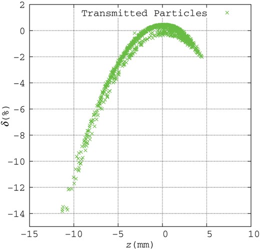
Positron distribution in longitudinal phase space at the end of the booster linac. Crosses show positrons passing through the booster linac.
To match the beam to the DR acceptance, the ECS is placed after the booster. The ECS consists of three L-band accelerator structures with a 20 MV/m accelerator gradient and an aperture 17 mm in radius. The transverse plane distribution after the ECS is shown in Fig. 13. Crosses show positrons passing through the ECS and the circle shows the aperture of the L-band accelerator. The positrons with |$|x|>0.035$| m were lost to consider the physical aperture of the beam duct at the chicane in the ECS. A comparison to Fig. 11 reveals that the beam size is enlarged by the ECS, and some positrons are over 10 mm from the center in the transverse plane. This result shows that some of the positrons are lost if we employ the S-band accelerator (10 mm aperture) instead of the L-band accelerator (17 mm aperture) in the ECS. Its beam size can be smaller by a proper shorter interval layout of the focusing quadrupoles between the accelerating structures in the ECS, and the S-band accelerator might be used there. This is beyond the scope of this report. The longitudinal phase-space distribution after the ECS is shown in Fig. 14. The ellipse in the figure shows the longitudinal aperture at the DR as it was defined in Eq. (1). The positron distribution is rotated and the energy deviation is compressed by the ECS. The compression ratio of |$\delta $| before the ECS to that after the ECS is about 3. Figures 15 and 16 are histograms about |$\delta $| before and after the ECS, respectively. The histogram in Fig. 15 has a long tail to |$-\delta $|, which will be lost without the ECS since the DR acceptance of |$\delta $| is less than 0.015 at full width. Figure 16 shows that all transmitted particles can be accepted in the DR acceptance of |$\delta $|.
Positron distribution in the transverse plane at the end of the ECS. Crosses show positrons passing through the ECS.
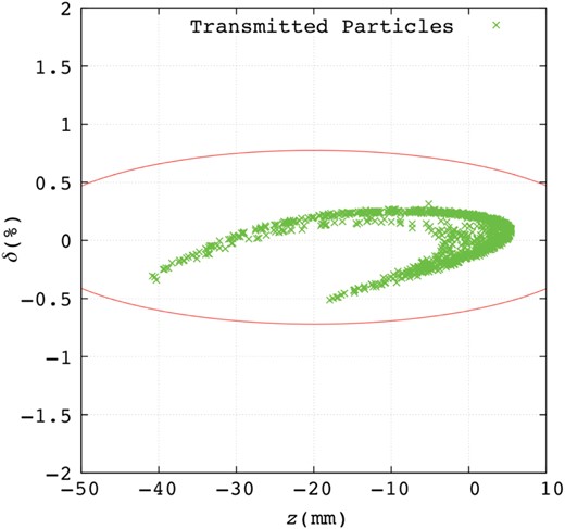
Positron distribution in longitudinal phase space at end of the ECS. Crosses show positrons passing through the ECS.
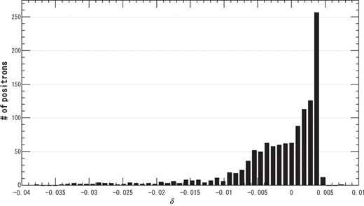
Histogram about |$\delta $| before the ECS.
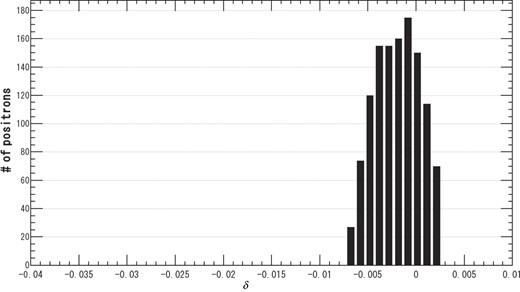
Histogram about |$\delta $| after the ECS.
After the ECS, the positron yield is defined as the ratio of the number of positrons accepted by the DR dynamic aperture to the number of electrons injected to the target. The ECS adds a gain of about 5–10% to the yield. Table 1 shows the parameter set optimized by the optimization procedure described in the next section.
An optimized parameter set. Aperture values indicate the radius.
| Parameter | Value | Unit |
|---|---|---|
| Drive beam energy | 6.0 | GeV |
| Target thickness | 14 | mm |
| Beam size (RMS) | 4.0 | mm |
| AMD peak field | 5.0 | T |
| AMD aperture | 8 | mm |
| Accelerator gradient (capture linac) | 25 | MV/m |
| Accelerator gradient (booster, ECS) | 20 | MV/m |
| Capture linac L-band accelerator aperture | 20 | mm |
| Booster and ECS L-band accelerator aperture | 17 | mm |
| Booster S-band accelerator aperture | 10 | mm |
| Solenoid field | 0.5 | T |
| PEDD | 27 | J/g |
| # of electrons as drive beam per bunch | 2.3 | |$10^{10}$| |
3.2. Parameter optimization
The parameters in the previous section were optimized by the following procedure:
RF phase of the capture linac and booster linac
Aperture of the booster linac and ECS
AMD peak field and aperture
Bending magnet angle and length in the chicane
Number of S-band accelerators in the booster linac
Drive-electron linac energy, target thickness, and electron beam size impinging on the target
These parameters were optimized to obtain a sufficient number of positrons in the DR acceptance. One of the parameters was varied to find the optimal value. The parameter was then set to the optimal value, and the remaining parameters were optimized one by one, with the previous parameters fixed. Optimization was performed to maximize the yield defined by the DR acceptance. The optimization was done by keeping the PEDD lower than 35 J/g. Cost effectiveness was also considered.
First, the RF phases in both the capture linac and the booster linac were optimized. The phases of all the RF cavities in the capture linac were the same. This is true for the positron booster, but the phases for the capture linac and the booster could differ. Figure 17 shows the yield as a function of the RF phase of the capture linac. Here, we define the yields at different locations and under different conditions. The circles show the yield defined at the end of the capture linac. All the positrons that arrive there are counted. The definition is similar for the crosses, which show the yield at the end of the ECS. The triangles show the yield at the end of the ECS considering the transverse DR acceptance. The squares show the yield at the end of the ECS considering both the transverse and longitudinal DR acceptance. For each capture linac RF phase, the phase of the booster linac is adjusted for the maximum yield at DR injection. The yield curves in the figure show two peaks around 50|$^{\circ }$| and 290|$^{\circ }$|, which correspond to the acceleration capture and deceleration capture regimes, respectively. In acceleration and deceleration capture, the bunch is located on the acceleration and deceleration phases at the entrance of the capture linac, respectively. In the deceleration phase, the bunch head is decelerated and slips down to the accelerator phase owing to the velocity modulation and spiral motion in the solenoid field. As a result, positrons are bunched at the acceleration phase. This bunching effect is not expected for acceleration capture. Therefore, deceleration capture has a better yield than acceleration capture, and the yield is more stable under phase deviation, as shown in Fig. 17. Deceleration capture is studied and its advantage is also proved in Ref. [28]. According to the simulation, 290|$^{\circ }$| is the optimal value of the RF phase. In the following procedures, the optimal value was used. In the optimal phase, about 20% of the positrons are lost as they pass through the booster linac. This is the other large difference from the result in Ref. [16], which ignored the booster acceleration. The values indicated by the crosses are almost the same as those indicated by the triangles, demonstrating that the ECS is effective.
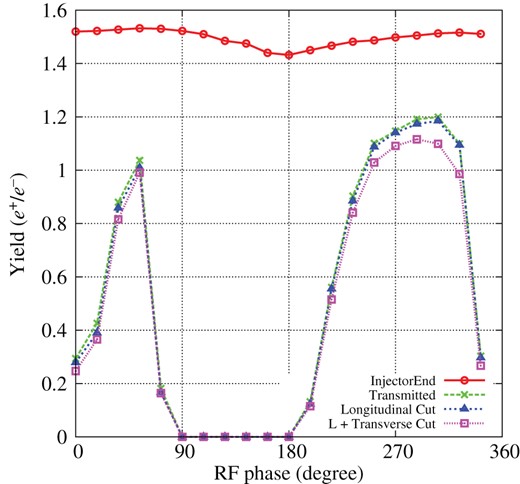
Yield as a function of the RF phase of the capture linac. Circles, crosses, triangles, and squares show the yields defined at different locations and conditions: end of the capture linac, end of the ECS, end of the ECS with longitudinal DR acceptance, and end of the ECS with transverse and longitudinal DR acceptance, respectively.
Second, the apertures of the booster linac and ECS were optimized. At this point, all the accelerating structures are in the L-band. Later, we try to replace the latter part of the booster linac with S-band structures having a smaller aperture (10 mm in radius) for better cost effectiveness. To examine the effect, we set several physical apertures, which appear in the simulation as a circular hole along the beam line. Positrons passing outside of the circular hole are removed from the simulation. Figure 18 shows the yield at the DR as a function of the radius aperture. A larger aperture gives a better yield, as expected, but the yield is saturated above 16 mm. A smaller aperture provides a better effective acceleration because it yields a higher acceleration field owing to the smaller group velocity. The optimal value of the radius aperture in the booster linac is 17 mm. In the following simulations, we used this value.
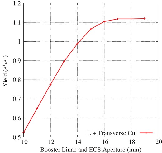
Yield as a function of the radius aperture in the booster linac and ECS.
Third, the AMD peak field and the aperture were optimized. Figure 19 shows the yield as a function of the AMD radius aperture for four peak AMD magnetic fields. Squares, circles, crosses, and triangles show the results for 3.0, 5.0, 7.0, and 9.0 T peak fields, respectively. Although a larger radius aperture gives a better yield, as expected, an aperture larger than 8 mm provides only a small gain, especially for the 5.0, 7.0, and 9.0 T peak fields. From the engineering viewpoint, a smaller aperture is better because a strong field can be easily induced. Among the various configurations, the 5.0 T peak field with an 8 mm aperture is optimal. In the following simulations, these optimal values were used.
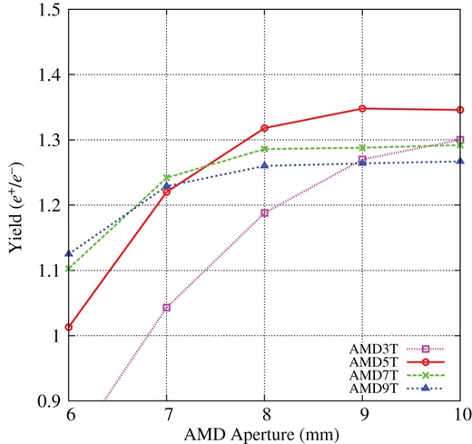
Yield as a function of AMD aperture for 3.0 T (squares), 5.0 T (circles), 7.0 T (crosses), and 9.0 T (triangles) peak fields. Aperture values indicate the radius.
Fourth, the chicane section was optimized. In this study, the chicane was introduced at the entrance of the booster linac. To optimize the bending angle and length of the chicane section, the yield was scanned for bending angles and various lengths, as shown in Fig. 20. Among the results, a bending angle of 0.21 rad and length of 0.48 m show the maximum yield at the end of the ECS. In the following simulations, a chicane with these optimum values was installed.
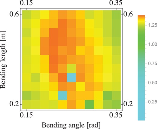
Yield as a function of bending angle and length; see legend on the right for color definitions.
Fifth, we tried to replace some L-band accelerating structures in the booster linac with S-band structures because the S-band accelerating system is less costly and more feasible than the L-band system owing to its technical maturity. The booster linac consists of 40 lattice cells, as mentioned in Sect. 2.5. We tried to replace the later part of the booster linac lattice cells with S-band accelerators. We assume that the accelerator gradient is the same for the L-band and S-band structures, but the radius of the physical aperture is 17 mm for the L-band and 10 mm for the S-band. Figure 21 shows the yield as a function of the lattice cell number at which the L-band lattice cells end. The figure shows that the yield decreases when we introduce the S-band accelerators, and the yield loss depends on the number of S-band structures. As we will show later, a yield of 1.28 provides sufficient positrons; i.e., after the 25th lattice cell, the booster can be implemented with S-band accelerators. In this configuration, the booster linac consists of 62 L-band RF cavities and 54 S-band RF cavities; i.e., about half of the RF cavities in the booster linac can be replaced by S-band RF cavities. In the following final procedure, we used this configuration; i.e., after the 25th lattice cell, the accelerator aperture is 10 mm in radius.
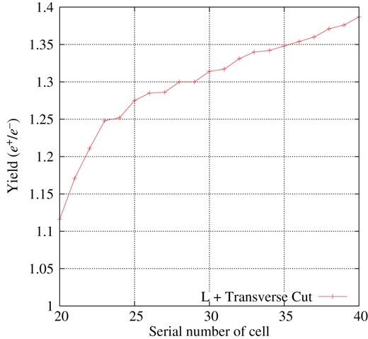
Yield as a function of the lattice cell number at which the L-band lattice cells end.
Finally, the drive-electron linac energy, target thickness, and electron beam size impinging on the target were optimized. Changing these parameters causes the PEDD and total energy deposition per bunch to vary. To compare the performance of these different configurations, the bunch intensity of the drive electron beam is adjusted to give the same number of positrons (|$3.0\times 10^{10}/$|bunch) in the DR acceptance. In other words, the PEDD and energy deposition are normalized by the number of captured positrons. In Fig. 22, the results are plotted in the PEDD per triplet (horizontal axis) and total energy deposition per bunch (vertical axis) plane. Blue circles show the results of a 3 GeV electron driver with 14 mm target thickness, red squares are of a 6 GeV driver with 14 mm thickness, and green triangles are of a 6 GeV driver with 20 mm thickness. The numbers associated with each point show beam spot in RMS (mm). As a practical limit based on the SLC [14], the PEDD should be less than 35 J/g to prevent any target destruction. The vertical red line shows the practical limit, and all points to the right of the line are excluded. There is no clear threshold for the energy deposition per bunch; however, a lower value is better. Among these configurations, a drive beam energy of 6 GeV, target thickness of 14 mm, and RMS spot size of 4 mm seem to be the optimal conditions. In this configuration, the drive beam intensity is |$2.3\times 10^{10}$| electrons per bunch, and a yield of 1.25 gives |$3.0\times 10^{10}$| positrons per bunch in the DR acceptance. In this case, the PEDD is 27 J/g, which is below the practical limit of 35 J/g.
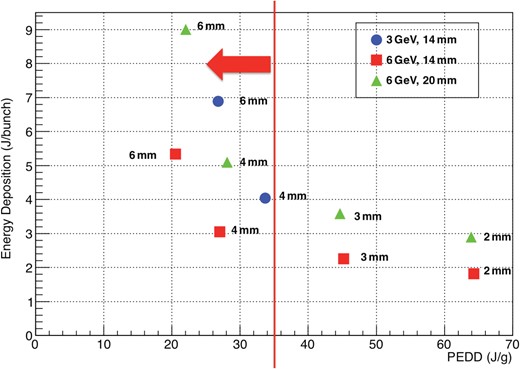
Data points are plotted in the plane of PEDD and energy deposition per bunch. PEDD and the energy deposition are normalized, giving 1.5 positrons per electron. Circles, squares, and triangles show the results of a 3 GeV driver and 14 mm target thickness, 6 GeV and 14 mm thickness, and 6 GeV and 20 mm thickness, respectively. Numbers associated with the points are the beam spot on the target in RMS. The red line shows the practical limit on PEDD of 35 J/g.
4. Summary
A start-to-end simulation of the ILC electron-driven positron source was performed. By including the energy spread caused by acceleration due to the RF curvature, the ECS has a crucial role in obtaining sufficient positrons. As a result of optimization, |$3.0\times 10^{10}$| positrons per bunch are obtained in the DR acceptance with a PEDD of 27 J/g on the target, which is less than the practical limit, 35 J/g. The driver linac has an energy of 6 GeV and |$2.3\times 10^{10}$| electrons per bunch. The target thickness is 14 mm, and the RMS beam size on the target is 4 mm. The yield (number of captured positrons per electron) is 1.25. The AMD peak field is 5.0 T for a radius aperture of 8 mm, which is technically reasonable. The booster linac can be a hybrid of L-band and S-band accelerators for cost effectiveness.
The parameters determined by the simulation are not extraordinary, and the system can be implemented without any technical difficulties. This electron-driven scheme can be a technical backup for the ILC positron source and improves the technical reliability of the ILC project.
In this simulation, beam-loading effects are ignored. To improve confidence in the simulation, the beam-loading effect should be included; this is an issue for future work.
Acknowledgments
This work was partially supported by a Grant-in-Aid for Scientific Research (C 26400293).
