


Abstract
Motivated by the possible existence of string axions with ultralight masses, we study gravitational radiation from an axion cloud around a rotating black hole (BH). The axion cloud extracts the rotation energy of the BH by superradiant instability, while it loses energy through the emission of gravitational waves (GWs). In this paper, GWs are treated as perturbations on a fixed background spacetime to derive the energy emission rate. We give an analytic approximate formula for the case where the axion Compton wavelength is much larger than the BH radius, and then present numerical results without approximation. The energy loss rate of the axion cloud through GW emission turns out to be smaller than the energy gain rate of the axion cloud by superradiant instability until nonlinear self-interactions of axions become important. In particular, an axion bosenova must happen at the last stage of superradiant instability.
1. Introduction
Within a few years, the ground-based detectors Advanced LIGO, Advanced VIRGO, and KAGRA are expected to begin operation with sufficiently high sensitivity to detect gravitational wave (GW) signals from binary mergers of black holes (BHs) or neutron stars. We will have a very exciting era of general relativity, and much interesting science will be done. One interesting possibility is finding signals from unknown sources or effects of unestablished hypothetical theories.
Do we have a possibility of detecting signals from string theory through GW detectors? Naïvely, it seems difficult because the effects of string theory are expected to appear at very high energy scales (e.g., the string scale). However, the authors of Refs. [1,2] answered “Maybe yes,” if there are string axions with ultralight masses. Since string theories (or M-theory) require our spacetime to have 10 or 11 dimensions, the extra dimensions beyond four have to be compactified. Then, the extra dimensions have dynamical degrees of freedom to change their shape and size which are called moduli, and they effectively behave as fields in our four-dimensional spacetime. One of the moduli will be the QCD axion. We can also expect the existence of other pseudoscalar fields with ultralight masses, called string axions, whose expected number is typically from 10 to 100. The allowed mass range is from |$10^{-10}$| eV to |$10^{-33}$| eV, and further below. Depending on their masses, they cause a variety of phenomena that could be observed in the context of cosmophysics (|$=$| cosmology and astrophysics). This is called the axiverse scenario (see also Ref. [3] for an overview).
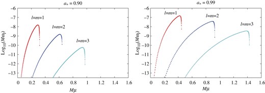
Imaginary part |$M\omega _{{\mathrm {I}}}$| of bound state eigenfrequency as functions of |$M\mu $| for the BH rotation parameter |$a_*=0.90$| (left) and |$0.99$| (right). The results for the modes |$\ell =m=1$|, |$2$|, and |$3$| are shown.
Suppose one of the string axions has mass |$\mu \sim 10^{-10}$| eV. The Compton wavelength |$1/\mu $| is comparable to the radius of a BH with solar mass |$M\sim M_{\odot }$| (throughout this paper, we use the units |$c=G=\hbar = 1$|). Then, around a rotating solar-mass BH, there appears an unstable quasi-bound-state mode whose amplitude grows exponentially through the extraction of the BH rotation energy. This instability is called superradiant instability. Due to this instability, an axion cloud is formed around the BH from quantum zero-point oscillations even if we start from vacuum. Assuming the behavior of the scalar field to be |$\Phi \propto {\mathrm {e}}^{-{\mathrm { i}}\omega t}$|, the growth rate has been calculated by approximate methods [4–6] and by numerical methods [7–9] by solving the frequency-domain eigenvalue problem (see also Ref. [10] for a related issue and Ref. [11] for recent simulations of the same system including gravitational backreaction).1 There, eigenfrequencies with complex values, |$\omega = \omega _{{\mathrm {R}}}+{\mathrm { i}}\omega _{{\mathrm { I}}}$|, are obtained, and a quasibound state is unstable if |$\omega _{{\mathrm {I}}}$| is positive. The maximum growth rate has been found to be |$M\omega _{{\mathrm {I}}}\sim 10^{-7}$|, and the corresponding time scale to be around |$10^{7} M$|, which is much longer than |$M$| (see Fig. 1). But this time scale is about |$1$| minute for |$M=M_{\odot }$|. Even for |$M\omega _{{\mathrm {I}}} \sim 10^{-12}$|, the time scale is about |$1$| day. Therefore, for a wide range of parameters, the time scale of the superradiant instability is much shorter than the observation period of the ground-based GW detectors.
The axion cloud becomes denser and denser as the superradiant instability proceeds, and two effects gradually become important. One is nonlinear self-interaction, and the other is the GW emission. Here, the nonlinear self-interaction comes from the potential of the axion field |$\Phi $|, which is assumed to have the standard form |$V = f_{{\mathrm {a}}}^2\mu ^2[1-\cos (\Phi /f_{{\rm a}})]$| in the present paper, where |$f_{{\mathrm {a}}}$| is the axion decay constant. In our previous paper [12], we numerically simulated the time evolution of an axion field obeying the sine–Gordon equation in the Kerr background spacetime. The result is that the nonlinear self-interaction leads to “axion bosenova,” which shares some features with the bosenova observed in experiments [15] on Bose–Einstein condensates. The bosenova is characterized by the termination of superradiant instability and the gradual infall of positive energy from the axion cloud into the BH. The bosenova happens when the energy |$E_{{\mathrm {a}}}$| of the axion cloud becomes |$E_{{\rm a}}/M\approx 1600(f_{{\mathrm {a}}}/M_{{\mathrm { p}}})^2$|, where |$M_{{\mathrm {p}}}$| is the Planck mass. If |$f_{{\mathrm {a}}}$| corresponds to the GUT scale, |$f_{{\mathrm {a}}}=10^{16}$| GeV, the bosenova happens when the axion cloud acquires 0.16% energy of the BH mass.
Approximate estimates of GW emissions from the BH–axion system were previously given by Arvanitaki et al. in Refs. [1,2]. There, the GW radiation from a huge gravitational atom in Newton potential was considered for the case |$M\mu \ll 1$|. Two GW emission processes were pointed out. One is radiation by level transitions of the axion cloud as a gravitational atom. This process occurs when the wavefunction of the axion cloud is given by the superposition of two or more levels of bound eigenstates, and GWs of frequencies identical to the energy differences of the levels are radiated. The other is the annihilation of two axions. This can happen even for an axion cloud occupying just one bound-state level, and GWs with the frequency |$2\omega $| are emitted, where |$\omega $| is the (real part of) the axion bound-state frequency. For both processes, Arvanitaki et al. derived approximate formulas for the GW radiation rates and concluded that the radiation rates are sufficiently small to allow the growth of the axion cloud by superradiant instability until the occurrence of a bosenova.
In this paper, we consider the situation where approximately all of the axion particles occupy one bound-state level. Because the GW radiation by level transition is subdominant in such a situation, we focus on the two-axion annihilation process. We push forward the study of Ref. [2] on this process in two respects. First, since the approximate analysis in Ref. [2] was limited to the case where the two axions to be annihilated are at the |$2p$| level (i.e., |$\ell =m=1$| and |$n_{{\mathrm {r}}}=0$|), we extend to more general cases of |$\ell =m\ge 1$| and |$n_{{\mathrm {r}}}\ge 0$|. Next, we perform numerical calculations of the GW emission in the Kerr background for general values of |$M\mu $|. This is certainly necessary because the superradiant instability for the modes |$\ell =m=2$| and |$3$| becomes effective when |$M\mu \sim 1$|, where the approximation |$M\mu \ll 1$| breaks down. Similarly to Ref. [2], the analysis is done within the classical approximation.
This paper is organized as follows. In the next section, we describe the general strategy and derive formulas that are used in the subsequent two sections. In Sect. 3, we give an approximate formula for the energy loss rate in the case |$M\mu \ll 1$|. In this case, the flat spacetime can be adopted as the background spacetime, and we call this approximation the “flat approximation.” In Sect. 4, we explain the numerical method for the general value of |$M\mu $|, where the Kerr spacetime is adopted as the background spacetime. Section 5 is devoted to the conclusion. In Appendix A, we describe technical details for computing axion quasi-bound states around a Kerr BH numerically. In Appendix B, we sketch the derivation of the GW radiation rate presented in Sect. 3.
2. General strategy
In this section, we briefly summarize the basic features of the superradiant growth of an axion cloud around a rotating BH and the methods for evaluating the GW radiation rate from this system.
2.1 Superradiant bound states of an axion field
The superradiant instability occurs only for quasi-bound states. Such a quasi-bound state is obtained by assuming the field to decay at infinity and to be ingoing at the horizon. The procedure is similar to the calculation of the bound states of a hydrogen atom in quantum mechanics. In the case of the hydrogen atom, one imposes the wave function to decay at infinity and to be regular at the origin. Then, the energy levels are discretized. In the same manner, the frequency |$\omega $| is discretized in the case of the BH–axion system. Since there is an ingoing flux at the horizon, the frequency |$\omega $| becomes complex, |$\omega = \omega _{{\mathrm {R}}} + {\mathrm { i}}\omega _{{\rm I}}$|. The imaginary part gives the exponential behavior: the field decays for |$\omega _{{\mathrm {I}}}<0$| and grows for |$\omega _{{\mathrm {I}}}>0$|. In the case |$\omega _{{\rm I}}>0$|, the bound state is unstable, and this happens when the superradiance condition |$\omega _{{\mathrm {R}}}<m\Omega _{{\rm H}}$| is satisfied. Physically, the instability happens because the energy density in the neighborhood of the BH horizon becomes negative for |$\omega _{{\rm R}}<m\Omega _{{\mathrm {H}}}$|, and negative energy falls into the horizon. Then, due to energy conservation, the amplitude of the outside field becomes larger. This is the superradiant instability.
Approximate solutions for superradiant bound states were constructed in the parameter region |$M\mu \ll 1$| by the matched asymptotic expansion (MAE) method [4], and in the parameter region |$M\mu \gg 1$| by the WKB method [5]. The solution in the MAE method is closely related to our analysis in Sect. 3. In this method, two approximate solutions are constructed in a near-horizon region and in a distant region, and they are matched in the overlapping region where both approximations are valid. The equation in the distant region is identical to the Schrödinger equation for a hydrogen atom except that the electric potential |$-e^2/r$| is replaced by the Newton potential |$-M\mu /r$|. Therefore, the BH–axion system can be regarded as a huge gravitational atom, which is characterized by the angular quantum numbers |$(\ell , m)$| and the radial quantum number |$n_{{\mathrm {r}}}=0, 1, 2, \ldots $|
In the parameter range |$M\mu \sim 1$|, numerical calculations are required to determine the bound-state levels. Such analyses have been done by several authors [7–9]. In Ref. [9], a detailed analysis was reported using the continued fraction method developed by Leaver [16]. We also reproduced a consistent result using our independent code—see Appendix A for technical details. For a quasi-bound state, the real part |$\omega _{{\mathrm {R}}}$| of the eigenfrequency is smaller than the mass |$\mu $|. The difference between the two quantities, |$\mu -\omega _{{\rm R}}$|, can be interpreted as the binding energy due to gravitational interaction, and typically the binding energy |$\mu -\omega _{{\mathrm {R}}}$| is found to be much smaller compared to the mass |$\mu $|. Figure 1 shows the numerical results for the imaginary part |$M\omega _{{\mathrm {I}}}$| of the eigenfrequency as functions of |$M\mu $| for the BH rotation parameter |$a_*=0.90$| and |$0.99$|. The results for the modes |$\ell = m = 1, 2,$| and |$3$| and |$n_{{\mathrm {r}}}=0$| are shown. The unstable range of |$M\mu $| becomes larger as |$m$| is increased because of the superradiance condition |$\mu \approx \omega _{{\mathrm {R}}}<m\Omega _{{\mathrm { H}}}$|. The peak value of |$M\omega _{{\mathrm {I}}}$| becomes smaller as |$\ell =m$| is increased and as |$a_*$| is decreased.
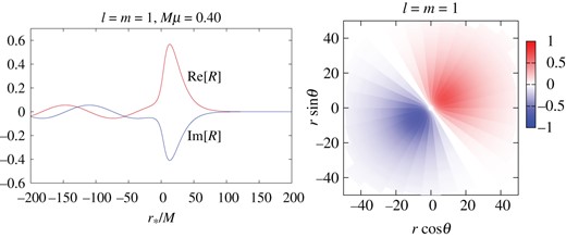
Left panel: Radial function |$R$| of the axion quasi-bound state as a function of the tortoise coordinate |$r_*/M$| for |$\ell = m = 1$|, |$M\mu = 0.40$|, and the BH rotation parameter |$a_*=0.99$|. Right panel: The configuration in the equatorial plane |$\theta =\pi /2$|. There is one maximum and one minimum.
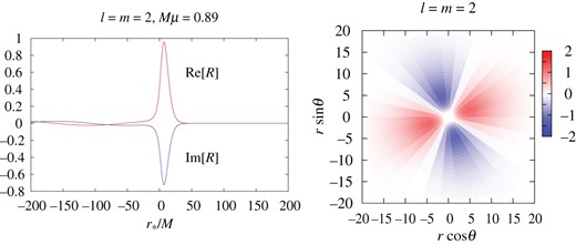
As Fig. 2 but for |$\ell = m = 2$| and |$M\mu = 0.89$|. We can see two maxima and two minima in the right panel.
2.2 GWs from an axion cloud
Here, we introduce one approximation. The field |$\Phi $| is proportional to |${\mathrm {e}}^{\omega _{{\mathrm { I}}} t}$| by the superradiant instability, and the energy–momentum tensor gradually grows larger. However, the time scale of the instability is very long, |$\gtrsim 10^7M$|, and its effect on the GW flux must be small. For this reason, we ignore the imaginary part |$\omega _{{\mathrm {I}}}$| and calculate GWs from an oscillating source without exponential growth. This also means that we ignore the ingoing flux of the field |$\Phi $| to the BH horizon.
In order to estimate the GW emission rate toward null infinity with the aid of the formula (17), in principle, we have to solve Eq. (11) first and then find a gauge transformation that puts the solution into the TT gauge. However, this is a rather intricate task. Therefore, we adopt the following different method.
Furthermore, in spite of the fact that the relation (26) was derived assuming the TT gauge conditions, the inner product |$\langle {u}^{(\tilde {j}){\rm TT}},{T}\rangle $| is invariant under the gauge transformation |$\hat {u}_{\mu \nu }^{{\mathrm {TT}}}\to \hat {u}_{\mu \nu }= \hat {u}_{\mu \nu }^{{\rm TT}}+\delta \hat {u}_{\mu \nu }$| with |$\delta \hat {u}_{\mu \nu } = \nabla _{\mu }\xi _{\nu } + \nabla _{\nu }\xi _{\mu }$| because |$\langle \delta u,T\rangle =0$| holds. This can be shown by rewriting the integral of |$(\nabla _{\mu }\xi _{\nu })T^{\mu \nu } = \nabla _{\mu }(T^{\mu \nu }\xi _{\nu })$| in the domain |$D$| into the surface terms by the Gauss law and using the absence of the energy flux at the boundaries |$r=r_{\mathrm {in}}$| and |$r_{\mathrm {out}}$|. Therefore, the inner product |$\langle \hat {u}^{(\tilde {j})},{T}\rangle $| can be calculated without taking special care of the gauge choice, and it is sufficient to find a solution |$u^{(\tilde {j})}_{\mu \nu }$| satisfying the TT gauge condition only at future null infinity. In the Kerr background, we can explicitly construct such out-mode solutions, as we will see later.
2.3 Methods for calculating the energy emission rate
In order to evaluate the radiation rate using Eq. (29), we have to calculate the homogeneous solution |$\hat {u}_{\mu \nu }$| for a gravitational perturbation and perform the integration of the inner product |$\langle u, T\rangle $|. Also, the values of |$J_{\tilde {j}}$| have to be calculated. We explain the methods for calculating these quantities.
2.3.1 Homogeneous GWs
2.3.2 Energy–momentum tensor
In the following two sections, we apply this formalism to the analytic approximation in the flat background spacetime and fully numerical calculations in the Kerr background spacetime, respectively.
3. Gravitational radiation in the flat approximation
3.1 Solution to Teukolsky equation
3.2 Energy emission rate
The remaining task is to obtain the homogeneous solution |$\hat {u}^{(\tilde {j})}_{\mu \nu }$| and calculate the integral |$\langle u^{(\tilde {j})}, T\rangle $|, where the index |$(\tilde {j})$| is a shorthand for |$(\tilde {\ell },\tilde {m}, P)$| to label each GW mode as noted in Sect. 2.2. Since the calculation of the inner product is rather tedious, we sketch the calculations in Appendix B, and just present the results here. It is convenient to discuss the results for the odd-type GWs (|$P=-1$|) and for the even-type GWs (|$P=+1$|) separately.
3.2.1 Odd-type perturbation
In the case of odd-type perturbation, |$P=-1$|, the inner product |$\langle u,T\rangle $| vanishes after integration with respect to the angular coordinates |$(\theta , \phi)$|. Therefore, we find that GWs of the odd-type modes are not radiated in our BH–axion system in the flat approximation. This is a natural result because the oscillating part of the energy–momentum tensor of the axion cloud has just the even-type mode. The stationary part of the energy–momentum tensor generates the odd-type perturbation that corresponds to the gravitational angular momentum, and this part has been ignored in our analysis.
3.2.2 Even-type perturbation
Approximate values of |$C_{n\ell }$|, values of |$Q_{\ell }$|, and the emitted GW mode |$(\tilde {\ell }, \tilde {m})$| for several axion cloud modes |$(n, \ell , m)$|.
| Axion mode |$(n,\ell ,m)$| | Atomic orbital | |$C_{n\ell }$| | |$Q_{\ell }$| | GW mode |$(\tilde {\ell },\tilde {m})$| |
|---|---|---|---|---|
| |$(2, 1, 1)$| | 2p | |$1.56\times 10^{-3}$| | |$14$| | |$(2, 2)$| |
| |$(3, 1, 1)$| | 3p | |$1.93\times 10^{-4}$| | |$14$| | |$(2, 2)$| |
| |$(4, 1, 1)$| | 4p | |$3.81\times 10^{-5}$| | |$14$| | |$(2, 2)$| |
| |$(3, 2, 2)$| | 3d | |$1.89\times 10^{-7}$| | |$18$| | |$(4, 4)$| |
| |$(4, 2, 2)$| | 4d | |$6.81\times 10^{-8}$| | |$18$| | |$(4, 4)$| |
| |$(5, 2, 2)$| | 5d | |$2.35\times 10^{-9}$| | |$18$| | |$(4, 4)$| |
| |$(4, 3, 3)$| | 4f | |$2.89\times 10^{-11}$| | |$22$| | |$(6, 6)$| |
| |$(5, 3, 3)$| | 5f | |$2.14\times 10^{-11}$| | |$22$| | |$(6, 6)$| |
| |$(6, 3, 3)$| | 6f | |$1.13\times 10^{-11}$| | |$22$| | |$(6, 6)$| |
| |$(5, 4, 4)$| | 5g | |$3.17\times 10^{-15}$| | |$26$| | |$(8, 8)$| |
| |$(6, 4, 4)$| | 6g | |$3.98\times 10^{-15}$| | |$26$| | |$(8, 8)$| |
| |$(7, 4, 4)$| | 7g | |$2.97\times 10^{-15}$| | |$26$| | |$(8, 8)$| |
3.3 Comparison with the superradiant growth rate
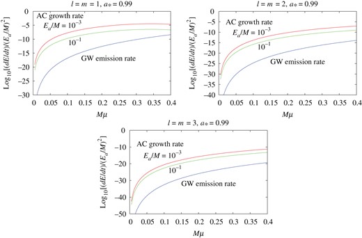
The GW radiation rate normalized by |$(E_{{\mathrm {a}}}/M)^2$| as functions of |$M\mu $| in the flat approximation. The cases of the axion cloud in the mode |$\ell = m = 1$|, |$2$|, and |$3$|, and |$n_{{\mathrm {r}}}=0$|, are shown for the BH rotation parameter |$a_*=0.99$|. The energy extraction rates of the axion cloud are also plotted for the two cases |$E_{{\mathrm {a}}}/M=10^{-3}$| and |$10^{-1}$| for comparison. In all cases, the energy extraction rate is larger than the GW radiation rate.
Figure 4 shows the GW radiation rate |${\rm d}E_{\mathrm {GW}}/{\mathrm { d}}t$| and the energy extraction rate |${\rm d}E_{{\mathrm {a}}}/dt$| by the superradiant instability normalized by |$(E_{{\mathrm {a}}}/M)^2$| as functions of |$M\mu $| for |$\ell =m=1$|, |$2$|, and |$3$|. The BH rotation parameter is fixed to be |$a_*=0.99$|, and we show the two cases where the energy of the axion cloud is |$E_{{\mathrm {a}}}/M\sim 10^{-3}$| and |$10^{-1}$|. These two values correspond to the energies when the bosenova happens for the choice of the decay constant |$f_{{\mathrm {a}}}=10^{16}$| and |$10^{17}$| GeV, respectively [12]. The figure shows that the energy extraction rate is much larger. For other values of the BH rotation parameter |$a_*$|, we have found that the result does not change in the region where the superradiant instability works effectively. Therefore, in the region |$M\mu \ll 1$|, the GW radiation rate is smaller than the energy extraction rate, and the GW emission does not hinder the growth of the axion cloud by the superradiant instability for a wide range of system parameters.
3.4 Reliability of the flat approximation
From the observations above, the value of the coefficients |$C_{n\ell }$| of Eq. (58c) is not reliable and may be changed by a factor. In fact, we also calculated the inner product |$\langle u, T\rangle $| using the gauge-invariant formalism for perturbations in spherically symmetric spacetimes in general dimensions [32] in the radiation gauge |$u_{0\mu }=u^{\mu }_{~\mu }=0$| and found that the prefactor |$C_{n\ell }$| for the radiation formula (58a) for the even-type mode differs from Eq. (58c) by a factor of |$(\ell -1)^2/4$| (although the result for the odd-type mode is unchanged). However, we would like to stress that the power dependence on |$(\mu M)$| must not be changed by the gauge choice: we can trust the power |$Q_{\ell }$| of |$(\mu M)$| given by Eq. (58b). We will confirm this statement in the fully numerical calculation in the Kerr background spacetime in the next section.
Note that this gauge dependence just appears in the case of the flat approximation. In the full numerical calculations in the Kerr background below, the gauge invariance of the inner product is guaranteed because the energy conservation |$\nabla _\mu T^{\mu \nu }=0$| is fully satisfied.
4. Gravitational radiation in Kerr background
In this section, we explain the numerical method of computing the GW radiation rate from an axion cloud in the Kerr background spacetime and present the numerical results. This analysis can be applied for the range of the system parameter |$M\mu \sim 1$|.
4.1 Numerical method
The numerical method of calculating the axion bound state |$\hat {\Phi }={\mathrm {e}}^{-{\rm i}\omega t}{\rm e}^{{\rm i}m\phi }R(r)S(\theta)$| was already explained in Sect. 2.1. The bound-state frequency and the radial function |$R(r)$| are obtained by the continued fraction method. The angular function |$S(\theta)$| is approximately calculated with an expansion formula |$S(\theta) = \sum _i S^{(i)}{c}_{0}^{i}$| with |${c}_{0}^2 = -a^2k^2$| up to the sixth order for each |$(\ell , m)$|—see Appendix A for details. Once these functions are obtained, the necessary components of the energy–momentum tensor are calculated with Eqs. (44a)–(44e).
In order to generate the homogeneous solutions |$u^{(\tilde {j})}_{\mu \nu }$|, we first calculate the functions and quantities that appear in the Teukolsky function—the spin-weighted spheroidal harmonics |${}_sS_{\tilde {\ell }\tilde {m}}^{~\tilde {\omega }}(\theta){\rm e}^{{\mathrm {i}}\tilde {m}\phi }$| and its eigenvalue |${}_sA_{\tilde {\ell }\tilde {m}}^{~\tilde {\omega }}$|, and the radial function |${}_sR_{\tilde {\ell }\tilde {m}}^{~\tilde {\omega }}(r)$|.
For the eigenvalue |${}_sA_{\tilde {\ell }\tilde {m}}^{~\tilde {\omega }}$|, we adopt the approximate formula for small |$\tilde {c}:=a\tilde {\omega }$| given in Refs. [33,34] that is applicable for arbitrary values of |$(s, \tilde {\ell }, \tilde {m})$|. This approximate formula is given in the form of the series expansion with respect to |$\tilde {c}=a\tilde {\omega }$| up to the sixth order. Since approximate formulas for the functions |${}_sS_{\tilde {\ell }\tilde {m}}^{~\tilde {\omega }}$| have not been given in the existing literature, we have derived the series expansion |${}_sS(\theta) = \sum _{i}{}_sS^{(i)}\tilde {c}^i$| up to the sixth order for each value of |$(s, \tilde {\ell }, \tilde {m})$|. The reason why we use the approximate formula is that regularization at poles is necessary when we calculate the metric from the Teukolsky functions. This regularization procedure is much more difficult for numerically generated data.
The radial function |${}_{+2}R_{\tilde {\ell }\tilde {m}}^{~\tilde {\omega }}(r_*)$| was numerically generated using the fourth-order Runge–Kutta method starting from |$r_*=-200$| to outward up to |$r_*/M = 1000$| or |$4000$| depending on the situation. Here, we choose |$s=+2$| for the following reason. In order to construct the out-mode solution, we have to generate solutions without ingoing waves that behave as |${}_{s}R_{\tilde {\ell }\tilde {m}}^{~\tilde {\omega }} \sim \Delta ^{-s}{\mathrm {e}}^{-{\rm i}(\tilde {\omega }-\tilde {m}\Omega _{{\rm H}})r_*}$| near the horizon. If we choose |$s=-2$|, the amplitude of ingoing waves is an exponentially increasing function of |$r_*$|, and therefore a small numerical error easily grows large to give a large amount of spurious ingoing waves in solving the equation from a near-horizon position to the outward direction. Conversely, in the case of |$s=+2$|, the amplitude of ingoing waves is an exponentially decreasing function, and a numerical error stays small to give a well-behaved solution. In other words, the out-mode solution is a numerical attractor for |$s=+2$|.
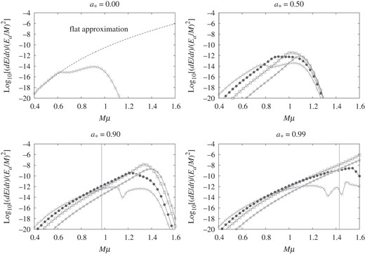
GW energy radiation rates for the modes |$(\tilde {\ell }, \tilde {m}) = (2,2)$| ( ), |$(3,2)$| (
 ), |$(4,2)$| (
 ), and |$(5,2)$| (
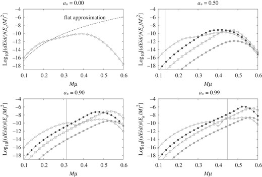
 ) from the axion cloud in the |$(\ell , m) = (1,1)$| mode as functions of |$M\mu $| in the cases of |$a_*=0.00$|, |$0.50$|, |$0.90$|, and |$0.99$|. The result for the flat approximation is shown by a dashed curve in the figure of |$a_*=0.00$|, and the vertical lines indicate the border of the superradiant instability for each |$a_*$|.
4.2 General properties
In the flat approximation in the previous section, all vector modes (|$P=-1$|) vanished. But in the case of the rotating Kerr background, our numerical data show that the |$P=-1$| modes are nonzero as we see below. The reason can be understood by considering the slow rotation case. The effect of the BH rotation is given by the odd-type perturbation, and the coupling between the even-type axion distribution and the odd-type rotation becomes the source for the odd-type GWs at the second order.
4.3 Numerical results
Now we show the numerical results.
4.3.1 |$\ell =m=1$|
We begin with the results for the axion cloud in the |$\ell = m = 1$| mode that is reduced to the gravitational atom with a vanishing radial quantum number |$n_{{\mathrm {r}}}=0$| for |$M\mu \ll 1$|. Figure 5 shows the GW radiation rates |${\mathrm {d}}E_{\rm GW}^{(\tilde {\ell }\tilde {m})}/{\rm d}t$| normalized by |$(E_{{\mathrm {a}}}/M)^2$| for the modes |$(\tilde {\ell }, \tilde {m})=(2,2)$| (circles,  ), |$(3,2)$| (black circles,
  ), |$(4,2)$| (squares,
  ), and |$(5,2)$| (black squares,
  ) as functions of |$M\mu $| for |$a_*=0.00$|, |$0.50$|, |$0.90$|, and |$0.99$|. Since GWs in the modes |$P=(-1)^{\tilde {\ell }+1}$| are not emitted, as discussed in Sect. 4.2, we just present the results for the modes |$P=(-1)^{\tilde {\ell }}$|. In the panel of |$a_*=0.00$|, only the mode |$(\tilde {\ell }, \tilde {m})=(2,2)$| is shown because other modes become zero for the same reason as the flat approximation. However, as the value of |$a_*$| is increased, the contribution of other modes becomes important. In fact, there are regions where the modes |$(\tilde {\ell }, \tilde {m})=(3,2)$| or |$(4,2)$| become dominant.
In each panel of |$a_*=0.50$|, |$0.90$|, and |$0.99$|, the vertical line indicates the threshold of the superradiant instability. On the left-hand side of the line, the axion cloud grows by superradiant instability, at least if the GW emission is neglected. On the right-hand side, no superradiant instability occurs, and the axion cloud, even if it were produced by some mechanism, would simply shrink gradually due to infall into the BH. We find the general tendency such that the radiation rate decreases for very large |$M\mu $|. The reason is as follows. In the superradiant regime, there is always a potential minimum of the axion field and the quasi-bound state is formed. Although this potential minimum also exists for |$M\mu $| not much larger than the threshold, it disappears at some point as |$M\mu $| is further increased. In such a situation, the field cannot form a bound state and it just falls into the horizon. Then, the field is concentrated near the horizon and the GW emission becomes inefficient, because the redshift effect becomes more and more significant as |$M\mu $| increases further. The GW radiation rate decreases rapidly with |$M\mu $|.
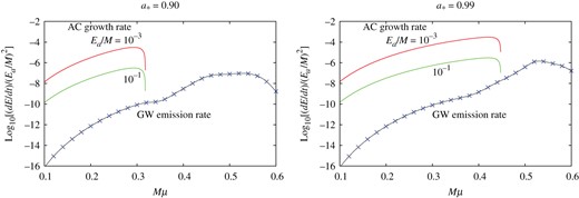
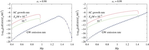
Total GW energy emission rate from the axion cloud in the |$(\ell , m) = (1,1)$| mode and the energy extraction rate of the axion cloud for the cases of |$E_{{\mathrm {a}}}/M=10^{-3}$| and |$10^{-1}$| as functions of |$M\mu $|. The cases of the BH rotation parameter |$a_*=0.90$| (left) and |$0.99$| (right) are shown. The total GW energy emission rate is evaluated by summing the first four GW modes |$\tilde {\ell } = 2$|, |$3$|, |$4$|, and |$5$|. The energy extraction rate is larger in all cases.
In the panel of |$a_*=0.00$|, the result of the flat approximation is also shown. For a small value of |$M\mu $|, our numerical data obey the same power dependence on |$M\mu $| as the approximate formula |${\mathrm {d}}E_{{\mathrm { GW}}}/{\rm d}t\propto (M\mu)^{14}$|. There is a shift by a constant factor from the curve of the approximate formula, because the value of |$C_{n\ell }$| includes the error by a factor as discussed in Sect. 3.4.
4.3.2 |$\ell =m=2$|
We turn our attention to the results for the axion cloud in the |$\ell = m = 2$| mode with the radial quantum number |$n_{{\mathrm {r}}}=0$|. Figure 7 shows the radiation rates |${\mathrm {d}}E_{\rm GW}^{(\tilde {\ell }\tilde {m})}/{\rm d}t$| normalized with |$(E_{{\mathrm {a}}}/M)^2$| for the GW modes |$(\tilde {\ell }, \tilde {m})=(4,4)$| (circles,  ), |$(5,4)$| (black circles,
  ), |$(6,4)$| (squares,
  ), and |$(7,4)$| (black squares,
  ) as functions of |$M\mu $| for |$a_*=0.00$|, |$0.50$|, |$0.90$|, and |$0.99$|. Similarly to the case |$\ell = m= 1$|, only the mode |$(\tilde {\ell }, \tilde {m})=(4,4)$| is radiated in the case of |$a_*=0.00$|. But as the value of |$a_*$| is increased, the contribution of other modes becomes important, and there are regions where the modes |$(\tilde {\ell }, \tilde {m})=(5,4)$| or |$(6,4)$| become dominant. Again, the effect of nonlinearity with respect to |$M\mu $| tends to suppress the GW radiation rate. Similarly to the case of |$\ell =m=1$|, the numerical data (shown in the panel of |$a_*=0.00$|) have the same power dependence |${\mathrm {d}}E_{\rm GW}/{\mathrm { d}}t \propto (M\mu)^{18}$| as the result of the flat approximation for |$M\mu \ll 1$|.
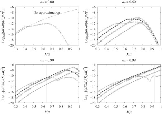
As Fig. 5 for the GW modes |$(\tilde {\ell }, \tilde {m}) = (4,4)$| ( ), |$(5,4)$| (
 ), |$(6,4)$| (
 ), and |$(7,4)$| (
 ) from the axion cloud in the |$\ell = m = 2$| mode.
Figure 8 compares the total GW radiation rate with the energy extraction rate as functions of |$M\mu $| for |$a_*=0.90$| and |$0.99$|. Here, the total GW radiation rate is approximated by the sum of the GW radiation rates for the first four modes with respect to |$\tilde {\ell }$|, and the curves of the energy extraction rate for the cases |$E_{{\rm a}}/M=10^{-3}$| and |$10^{-1}$| are shown. Similarly to the case |$\ell = m = 1$|, the GW radiation rate is much smaller than the energy extraction rate except for a very small region near the threshold of the superradiant instability. Therefore, the GW emission scarcely affects the growth of the axion cloud due to the superradiant instability also in the case |$\ell = m = 2$|.
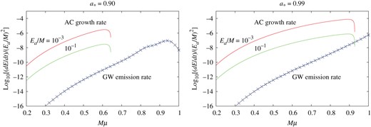
As Fig. 6 but for the axion cloud in the |$\ell = m = 2$| mode. The total GW energy radiation rate is evaluated by summing the first four GW modes |$\ell = 4$|, |$5$|, |$6$|, and |$7$|.
4.3.3 |$\ell =m=3$|
Finally, we show the results for the axion cloud in the |$\ell = m = 3$| mode with the radial quantum number |$n_{{\rm r}}=0$|. Figure 9 shows the radiation rates |${\rm d}E_{\mathrm {GW}}^{(\tilde {\ell }\tilde {m})}/{\rm d}t$| normalized by |$(E_{{\mathrm {a}}}/M)^2$| for the GW modes |$(\tilde {\ell }, \tilde {m})=(6,6)$| (circles,  ), |$(7,6)$| (black circles,
  ), |$(8,6)$| (squares,
  ), and |$(9,6)$| (black squares,
  ) as functions of |$M\mu $| for |$a_*=0.00$|, |$0.50$|, |$0.90$|, and |$0.99$|. The general features are same as the previous two cases. Although only the mode |$(\tilde {\ell }, \tilde {m})=(6,6)$| is radiated in the nonrotating case, the contribution of other modes becomes important as the value of |$a_*$| is increased. The GW radiation is suppressed for a very large value of |$M\mu $|. In this case, the numerical data coincide well with the flat approximation for |$M\mu \ll 1$|, as shown in the panel of |$a_*=0.00$|.
As Fig. 5 but for the GW modes |$(\tilde {\ell }, \tilde {m}) = (6,6)$| ( ), |$(7,6)$| (
 ), |$(8,6)$| (
 ), and |$(9,6)$| (
 ) from the axion cloud in the |$\ell = m = 3$| mode.
Figure 10 compares the total GW radiation rate (approximated by the sum of the radiation rates for the first four modes with respect to |$\tilde {\ell }$|) and the energy extraction rates for |$E_{{\mathrm {a}}}/M=10^{-3}$| and |$10^{-1}$| as functions of |$M\mu $| for |$a_*=0.90$| and |$0.99$|. Again, the GW radiation rate is much smaller than the energy extraction rate except for a very small region near the threshold of the superradiant instability.
As Fig. 6 but for the axion cloud in the |$\ell = m = 3$| mode. The total GW energy emission rate is evaluated by summing the first four GW modes |$\ell = 6$|, |$7$|, |$8$|, and |$9$|.
4.4 Summary of the numerical result
We have calculated the GW radiation rates to infinity, |${\mathrm {d}}E_{\rm GW}^{\rm (out)}/{\rm d}t$|, as functions of |$M\mu $| from the axion clouds in the modes |$\ell = m = 1$|, |$2$|, and |$3$|. Our numerical data have the same power dependence as the flat approximation for small values of |$M\mu $|. We compared the numerical results of |${\mathrm {d}}E_{\rm GW}/{\mathrm { d}}t$| with the energy extraction rates |${\rm d}E_{{\mathrm {a}}}/{\mathrm { d}}t$| of the axion cloud. The value of |${\mathrm {d}}E_{\rm GW}^{\rm (out)}/{\rm d}t$| is much smaller than |${\mathrm {d}}E_{{\mathrm { a}}}/{\mathrm { d}}t$| for both the cases |$E_{{\mathrm {a}}}/M=10^{-3}$| and |$10^{-1}$|. Therefore, similarly to the flat approximation, the axion cloud also grows by the superradiant instability until the effect of the nonlinear self-interaction becomes important when the background spacetime is adopted to be a rotating Kerr BH spacetime.
5. Conclusion
This formula cannot be used when |$\alpha _g$| becomes of the order of unity, because the axion cloud approaches the BH horizon and relativistic effects become significant. Therefore, for the parameter range |$\alpha _g \sim 1$|, we have computed the GW emission rate from the axion cloud corresponding to the modes |$\ell = m = 1$|, |$2$|, and |$3$| by solving the perturbation of the Kerr background spacetime numerically. As shown in Figs. 5, 7, and 9, the results of the numerical calculations indicate that the GW emission rate for each GW mode deviates from the above analytic formula when |$\alpha _g$| approaches unity, and rapidly decreases beyond some critical value of |$\alpha _g$| due to relativistic effects. This critical value of |$\alpha _g$| depends on the angular momentum parameter |$a_*=J/M^2$| and the quantum number |$\ell $| characterizing the superradiant mode of the cloud, and increases with |$a_*$| and |$\ell $|. Interestingly, up to this critical value, the above analytic formula reproduces the numerical results rather well when |$a_*$| is large if the energy emission rates of all modes are summed up, although the deviation becomes significant at larger |$\alpha _g$| for |$a_*\ll 1$|.
These GW emission rates were compared with the energy extraction rate by the superradiant instability. When the axion decay constant is in the range |$f_{{\rm a}}=10^{16}$|–|$10^{17}\,{\mathrm {GeV}}$| [12] and the angular momentum is in the range |$a_*=0.90$|–|$0.99$|, we have found that the GW emission rate is much smaller than the energy extraction rate except for a small region near the threshold of superradiant instability, as illustrated in Figs. 4, 6, 8, and 10. Therefore, the GW emission does not hinder the growth of the axion cloud through the superradiant instability for a wide range of the system parameters.
In our previous paper [12], we simulated the time evolution of an axion field around a Kerr BH taking account of nonlinear self-interaction, and showed that “axion bosenova” happens as the result of superradiant instability. Our results in this paper indicate that we do not have to change this picture even if we take into account the backreaction of the GW emission from the axion cloud. Since the GW emission rate is sufficiently low, the superradiant instability continues until the bosenova happens by nonlinear self-interaction.
In the present paper, we have studied the case in which only a single mode grows by superradiance. In realistic situations, however, there may exist several unstable modes. Although the instability growth rates for them are largely different, the amplitudes of all of them can become large simultaneously if the instability growth times are all shorter than the age of the BH. Then, GW emissions in the superradiant phase will be more complicated because the emitted GWs will be the superposition of those from the two-axion annihilation processes in several bound-state levels and from the process of axion level transitions. This multi-level occupation will also make the bosenova collapse and the associated GW emissions much more complicated. Further, we should also carefully estimate the detectability of GW emissions in the superradiant phase because it lasts for a much longer time than the bosenova collapse. Clearly, GW emissions in such realistic situations can be correctly evaluated only by combining the method developed in the present paper and the numerical simulations of bosenova in our previous paper [12]. This program is now in progress.
Acknowledgements
H.Y. thanks Masato Nozawa, Takahiro Tanaka, Yasumichi Sano, Misao Sasaki, and Kouji Nakamura for helpful comments. This work is supported by the Grant-in-Aid for Scientific Research (A) (22244030) from Japan Society for the Promotion of Science (JSPS).
Appendix A. Numerical construction of axion bound states
In this appendix, we present details of the numerical construction of the quasibound state of an axion cloud.
A.1 Equation
A.2 Angular eigenvalues and angular eigenfunctions
A.3 Continued fraction method
A.4 Radial function
Once the eigenfrequency |$\omega $| for the quasi-bound state is determined, we can numerically calculate the sequence of numbers |$a_n$| using the recurrence relations (A10a) and (A10b). Then, using the formula (A8), the radial function |$R(r)$| is generated. Some examples can be found in Figs. 2 and 3.
Appendix B. Inner product in the flat approximation
In Sect. 3, we presented the formula for the gravitational radiation rate. The radiation rate vanishes for the odd-type modes, and is given by Eqs. (58a)–(58c) for the even-type modes. These results are derived from Eqs. (43) and (57) after calculating |$\langle u, T\rangle $|. In this section, we sketch the calculation of this inner product |$\langle u, T\rangle $|.
For simplicity, we denote the radial function and spin-weighted spherical harmonics for the Teukolsky function as |$\tilde {R}:= {}_{+2}R_{\tilde {\ell }\tilde {m}}(r)$| and |${}_{s}\tilde {Y} := {}_{s}Y_{\tilde {\ell }\tilde {m}}(\theta ,\phi)$|, respectively. On the other hand, |$R=R_{\ell m}(r)$| and |$Y:=Y_{\ell m}(\theta ,\phi)$| represent the radial function and spherical harmonics for the axion field.
B.1 Odd-type modes
B.2 Even-type modes
The homogeneous GWs are classified into four independent modes: in-, out-, up-, and down-modes depending on the boundary conditions at future and past null infinity |$\mathscr {I}^+$| and |$\mathscr {I}^-$| and the future and past horizons |$\mathscr {H}^+$| and |$\mathscr {H}^-$| (see, e.g., p. 93 of Ref. [20]).
There is arbitrariness in the phase choice in the spin-weighted spherical/spheroidal harmonics that depends on authors, and our choice is different from that of Ref. [24]. We thank the referee of this paper for pointing this out.
The authors of Ref. [29] derived an apparently different formula and claimed that Chrzanowski's formula includes typos. However, we have checked that both the formulas lead to the same result.
References
